Complex Parameter Rao and Wald Tests for Assessing the Bandedness of a Complex-Valued Covariance Matrix

Abstract

Banding the inverse of a covariance matrix has become a popular technique for estimating a covariance matrix from a limited number of samples. It is of interest to provide criteria to determine if a matrix is bandable, as well as to test the bandedness of a matrix. In this paper, we pose the bandedness testing problem as a hypothesis testing task in statistical signal processing. We then derive two detectors, namely the complex Rao test and the complex Wald test, to test the bandedness of a Cholesky-factor matrix of a covariance matrix’s inverse. Furthermore, in many signal processing fields, such as radar and communications, the covariance matrix and its parameters are often complex-valued; thus, it is of interest to focus on complex-valued cases. The first detector is based on the complex parameter Rao test theorem. It does not require the maximum likelihood estimates of unknown parameters under the alternative hypothesis. We also develop the complex parameter Wald test theorem for general cases and derive the complex Wald test statistic for the bandedness testing problem. Numerical examples and computer simulations are given to evaluate and compare the two detectors’ performance. In addition, we show that the two detectors and the generalized likelihood ratio test are equivalent for the important complex Gaussian linear models and provide an analysis of the root cause of the equivalence.

1. Introduction

In statistical signal processing applications, such as radar and communications, the sample covariance matrix plays an essential role [1]. It is usually estimated from N sample data vectors $[{\mathbf{x}}_0{\mathbf{x}}_1\dots ,{\mathbf{x}}_{N-1}]$, where ${\mathbf{x}}_n$ is assumed to be $L\times 1$ identical and independently distributed (IID). The maximum likelihood covariance matrix estimate is [2]

$$\widehat{\mathbf{C}}=\frac{1}{N}\sum _{n=0}^{N-1}{\mathbf{x}}_n{\mathbf{x}}_n^H,$$

(1)

where H denotes a Hermitian. A good covariance matrix estimate usually requires the number of samples N to be sufficiently large. For instance, in space–time adaptive processing (STAP), it requires $N\ge 2L$ to have a good clutter covariance matrix estimate of size $L\times L$ [3]. In practice, however, this is not valid due to the nonstationary environment. For example, the data for a STAP system are often nonstationary due to the heterogeneous clutter [1]. The number of data that are sufficiently IID (homogeneous) can be relatively small $N\le L$ [3].

Techniques such as thresholding and banding are common ways to achieve better covariance matrix estimation. The thresholding method sets small elements of the sample covariance matrix to zero to obtain better estimators [4,5]. Another approach is to band or taper the sample covariance matrix [6,7]. Rothman et al. [8] proposed a Cholesky-based covariance regularization method to ensure positive definiteness. In practice, the inverse covariance matrix may be of primary interest. When the data are multivariate Gaussian, the inverse of the covariance matrix can be used to infer the conditional dependence structure of random variables [9].

Several researchers have investigated different methods for banding the inverse of the covariance matrix. Wu et al. proposed estimating the covariance matrix by banding the Cholesky-factor matrix and applying kernel smoothing estimation [10]. Bickel demonstrated that within the bandable class of covariance matrices, the estimator ${\widehat{\mathbf{C}}}^{-1}$ obtained by banding the Cholesky-factor matrix of the covariance matrix’s inverse is consistent [4,6]. Qian et al. explored adaptive banding covariance estimation for high-dimensional multivariate longitudinal data [11]. However, not much work is available to provide a criterion for deciding if a covariance matrix is bandable. Such a criterion would be useful for deciding if the banding technique is a suitable strategy in covariance matrix estimation tasks. Moreover, other covariance estimation methods, such as modeling the covariance matrix as a time-varying autoregressive moving average (ARMA) model [12], also require one to test if the model has a good fit, which is similar to but distinct from model order estimation techniques such as the minimum description length (MDL), AIC, BIC, and Bayesian exponential embedded family [13]. Some recent tests for bandedness can be found in [14], where a method for estimating matrix bandwidth is presented. Peng et al. developed several tests for sparse high-dimensional covariance matrices [15]. In [9], An et al. proposed test statistics for detecting band size and applied them to cancer data analysis. In contrast to these works, we pose the problem as a classical parameter hypothesis testing problem, which allows us to employ well-established detection theorems and algorithms in statistical signal processing.

In many practical fields, such as radar and communications, the data and parameters are often complex-valued [16]; therefore, we consider the bandedness testing problem for a complex-valued covariance matrix herein. Some general topics related to complex-valued signal processing can be found in [17,18]. In [19], Kay and Zhu derived the complex parameter Rao test, which allows one to develop a Rao test for complex parameters in a complex-valued domain directly. Based on [19], Sun et al. extended the complex parameter Rao test to include the case of nuisance parameters and also derived the Wald, Gradient, and Durbin tests for complex-valued parameters in a recently published paper [20]. In the present paper, we also derive the complex parameter Wald test as a parallel task and apply it to the problem of testing the bandedness of a covariance matrix.

The Rao test and Wald test are asymptotically optimal detectors for large data records. The complex parameter Rao test requires a lower computational cost than some other detectors, i.e., the generalized likelihood ratio test (GLRT) and Wald test. This is because it does not require the MLEs of unknown parameters under the alternative hypothesis $H_1$. This property can be desirable in high-dimensional multivariate signal processing [19], as low latency is a key performance indicator in such systems. The Rao test strikes a good balance between performance and computational cost. The complex parameter Rao test proposed by Kay and Zhu has been applied to multiple problems of radar and communication signal processing [19].

The Wald test is another very useful detector in addition to the Rao test. It is useful in radar target detection tasks, including but not limited to the detection of point targets, extended targets, and multiple-input/multiple-output radar targets in homogeneous, partially homogeneous, and heterogeneous environments [21,22]. In general, it is an equivalent large-data-record test that has the same asymptotically optimal detection performance as the GLRT and the Rao test. For finite-data records, however, it is not guaranteed to have the same performance as the GLRT [23,24,25,26]. In some cases, compared to the GLRT, the Wald test might be more robust when a mismatch exists and may have a lower computational complexity [22]. An example of its application can be found in adaptive detection for frequency diverse array multiple-input/multiple-output radar [27].

This paper is organized as follows: Section 2 formulates the problem of testing the bandedness of a covariance matrix; Section 3.1 derives the complex parameter Rao test detector for testing the bandedness of the Cholesky-factor matrix; and in Section 3.2, we derive the general complex Wald test for the complex-valued parameter hypothesis testing problem. In Section 3.2.3, the complex Wald test for the bandedness testing problem is derived. Examples and computer simulations for evaluating the Rao and Wald detector’s performance are given in Section 4. In addition, the equivalence between complex Wald and Rao tests for the ubiquitous complex Gaussian linear models is proved and analyzed in Section 4.2. Finally, conclusions are drawn in Section 5.

2. Problem Formulation

Assume that we have N IID observed data vectors, $\mathbf{X}={[{\mathbf{x}}_0^T{\mathbf{x}}_1^T\dots {\mathbf{x}}_{N-1}^T]}^T$, where T denotes transpose and each ${\mathbf{x}}_n$ is an $L\times 1$ complex-valued data vector conforming to a zero-mean multivariate complex Gaussian distribution ${\mathbf{x}}_n\sim \mathcal{CN}(\mathbf{0},\mathbf{C})$ for $n=0,1,\dots ,N-1$, and the ${\mathbf{x}}_n$s are mutually independent. In addition, we assume $N\le L$. The $L\times L$ covariance matrix $\mathbf{C}$ is a Hermitian matrix, so its inverse can be decomposed via the Cholesky decomposition as

$${\mathbf{C}}^{-1}={\mathbf{D}}^H\mathbf{D},$$

(2)

where $\mathbf{D}$ is a lower triangular $L\times L$ matrix. And it has a testing model as follows.

$$\mathbf{D}={\mathbf{D}}_B+\sum _{k=1}^M{b}_k{\mathbf{\Phi }}_k,$$

(3)

where ${\mathbf{D}}_B$ is a known banded lower triangular matrix, with a bandwidth of m, $b_k$’s are unknown complex-valued parameters, and ${\mathbf{\Phi }}_k$s are known basis matrices.

Specifically,

$$\begin{array}{ccc}\hfill b_1={\left[\mathbf{D}\right]}_{m+2,1},& \hfill & \hfill {\mathbf{\Phi }}_1={\mathbf{e}}_{m+2}{\mathbf{e}}_1^T\\ \hfill b_2={\left[\mathbf{D}\right]}_{m+3,2},& \hfill & \hfill {\mathbf{\Phi }}_2={\mathbf{e}}_{m+3}{\mathbf{e}}_2^T\\ \hfill ⋮& \hfill & \hfill ⋮\\ \hfill b_{N-m-1}={\left[\mathbf{D}\right]}_{N,N-m-1},& \hfill & \hfill {\mathbf{\Phi }}_{N-m-1}={\mathbf{e}}_N{\mathbf{e}}_{N-m-1}^T\\ \hfill b_{N-m}={\left[\mathbf{D}\right]}_{m+3,1},& \hfill & \hfill {\mathbf{\Phi }}_{N-m}={\mathbf{e}}_{m+3}{\mathbf{e}}_1^T\\ \hfill b_{N-m+1}={\left[\mathbf{D}\right]}_{m+4,2},& \hfill & \hfill {\mathbf{\Phi }}_{N-m+1}={\mathbf{e}}_{m+4}{\mathbf{e}}_2^T\\ \hfill ⋮& \hfill & \hfill ⋮\\ \hfill b_M={\left[\mathbf{D}\right]}_{N,1},& \hfill & \hfill {\mathbf{\Phi }}_M={\mathbf{e}}_N{\mathbf{e}}_1^T\end{array}$$

(4)

where $M=\frac{(N-m-1)(N-m)}{2}$ and ${\mathbf{e}}_k$ is an $L\times 1$ vector with its $k^{th}$ element being one and all other elements being zeros. The objective is to test whether the lower triangular Cholesky factor matrix $\mathbf{D}$ is equal to the banded lower triangular matrix ${\mathbf{D}}_B$. Let $\mathbf{b}={[b_1{b}_2\dots b_M]}^T$, then the detection problem is equivalent to choosing between the following two hypotheses:

$$\begin{array}{cc}\hfill {\mathcal{H}}_0:\mathbf{b}& =\mathbf{0};\hfill \\ \hfill {\mathcal{H}}_1:\mathbf{b}& \ne \mathbf{0};\hfill \end{array}$$

(5)

3. Methods

In this section, we derive the complex Rao test and the complex Wald test for the hypothesis testing problem stated above.

3.1. The Complex Rao Test for Testing the Bandedness

The Rao test attains asymptotic (as $N\to \infty$) performance as the GLRT, yet it circumvents the necessity of MLEs under the alternative hypothesis ${\mathcal{H}}_1$. As a result, so its computation cost can be lower than that of the GLRT, offering a desirable property in high-dimensional signal processing, including real-time STAP. Subsequently, we proceed by applying the complex Rao test theorem introduced in [19] to derive the Rao test statistic. Let ${\mathbf{b}}^{*}={[b_1^{*}{b}_2^{*}\dots b_M^{*}]}^T$, where ∗ denotes conjugate, and $\underline{\mathbf{b}}={\left[{\mathbf{b}}^T{\mathbf{b}}^H\right]}^T$, which is a $2M\times 1$ complex-valued parameter vector. The complex parameter Rao test detector can be formed according to [19]

$$T_R\left(\mathbf{X}\right)={\left.\frac{\partial lnp(\mathbf{X};\underline{\mathbf{b}})}{\partial {\underline{\mathbf{b}}}^{*}}\right|}_{\mathbf{b}=\mathbf{0}}^H{\left.{\mathbf{I}}^{-1}\left(\underline{\mathbf{b}}\right)\right|}_{\mathbf{b}=\mathbf{0}}{\left.\frac{\partial lnp(\mathbf{X};\underline{\mathbf{b}})}{\partial {\underline{\mathbf{b}}}^{*}}\right|}_{\mathbf{b}=\mathbf{0}}$$

(6)

where,

$$\frac{\partial lnp(\mathbf{X};\underline{\mathbf{b}})}{\partial \underline{\mathbf{b}}}={\left[{\frac{\partial lnp(\mathbf{X};\underline{\mathbf{b}})}{\partial \mathbf{b}}}^T{\frac{\partial lnp(\mathbf{X};\mathbf{b})}{\partial {\mathbf{b}}^{*}}}^T\right]}^T,$$

(7)

$$\frac{\partial lnp(\mathbf{X};\underline{\mathbf{b}})}{\partial \mathbf{b}}={\left[\frac{\partial lnp(\mathbf{X};\underline{\mathbf{b}})}{\partial b_1}\frac{\partial lnp(\mathbf{X};\underline{\mathbf{b}})}{\partial b_2}\dots \frac{\partial lnp(\mathbf{X};\underline{\mathbf{b}})}{\partial b_M}\right]}^T,$$

(8)

$$\frac{\partial lnp(\mathbf{X};\underline{\mathbf{b}})}{\partial {\mathbf{b}}^{*}}={\left[\frac{\partial lnp(\mathbf{X};\underline{\mathbf{b}})}{\partial b_1^{*}}\frac{\partial lnp(\mathbf{X};\underline{\mathbf{b}})}{\partial b_2^{*}}\dots \frac{\partial lnp(\mathbf{X};\underline{\mathbf{b}})}{\partial b_M^{*}}\right]}^T,$$

(9)

are based on Wirtinger derivatives. We can find each element, $\frac{\partial lnp(\mathbf{X};\mathbf{b})}{\partial b_k}$, as follows. First.

$$\begin{array}{cc}\hfill p(\mathbf{X};\underline{\mathbf{b}})& =\prod _{n=0}^{N-1}p({\mathbf{x}}_n;\underline{\mathbf{b}})\hfill \\ \hfill & =\prod _{n=0}^{N-1}\frac{1}{{\pi }^{L}det\left(\mathbf{C}\right)}exp(-{\mathbf{x}}_n^H{\mathbf{C}}^{-1}{\mathbf{x}}_n)\hfill \\ \hfill & =\frac{1}{{\pi }^{NL}{\prod }_{n=0}^{N-1}det\left(\mathbf{C}\right)}exp(-\sum _{n=0}^{N-1}{\mathbf{x}}_n^H{\mathbf{C}}^{-1}{\mathbf{x}}_n)\hfill \\ \hfill & =\frac{1}{{\pi }^{NL}}exp(-\sum _{n=0}^{N-1}{\mathbf{x}}_n^H{\mathbf{D}}^H\mathbf{D}{\mathbf{x}}_n)\prod _{n=0}^{N-1}det\left({\mathbf{D}}^H\mathbf{D}\right).\hfill \end{array}$$

(10)

Then,

$$\begin{array}{c}\hfill lnp(\mathbf{X};\underline{\mathbf{b}})=ln\left(\frac{1}{{\pi }^{NL}}\right)-\sum _{n=0}^{N-1}{\mathbf{x}}_n^H{\mathbf{D}}^H\mathbf{D}{\mathbf{x}}_n+Nlndet\left({\mathbf{D}}^H\mathbf{D}\right),\end{array}$$

(11)

and

$$\begin{array}{cc}\hfill \frac{\partial lnp(\mathbf{X};\underline{\mathbf{b}})}{\partial b_k}& =N\frac{\partial lndet\left({\mathbf{D}}^H\mathbf{D}\right)}{\partial b_k}-\sum _{n=0}^{N-1}\frac{\partial {\mathbf{x}}_n^H{\mathbf{D}}^H\mathbf{D}{\mathbf{x}}_n}{\partial b_k}\hfill \\ \hfill & =N\frac{\partial lndet\left({\mathbf{D}}^H\mathbf{D}\right)}{\partial b_k}-\sum _{n=0}^{N-1}\frac{\partial \mathrm{tr}\left(\mathbf{D}{\mathbf{x}}_n{\mathbf{x}}_n^H{\mathbf{D}}^H\right)}{\partial b_k},\hfill \end{array}$$

(12)

for $k=1,2,\dots ,M$, where

$$\begin{array}{cc}\hfill \frac{\partial lndet\left({\mathbf{D}}^H\mathbf{D}\right)}{\partial b_k}& =\mathrm{tr}\left({\mathbf{D}}^{-1}{\mathbf{\Phi }}_k\right),\hfill \end{array}$$

(13)

and

$$\begin{array}{c}\hfill \frac{\partial \mathrm{tr}\left(\mathbf{D}{\mathbf{x}}_n{\mathbf{x}}_n^H{\mathbf{D}}^H\right)}{\partial b_k}=\mathrm{tr}\left({\mathbf{x}}_n{\mathbf{x}}_n^H{\mathbf{D}}^H{\mathbf{\Phi }}_k\right).\end{array}$$

(14)

Thus,

$$\begin{array}{cc}\hfill \frac{\partial lnp(\mathbf{X};\underline{\mathbf{b}})}{\partial b_k}& =N\mathrm{tr}\left({\mathbf{D}}^{-1}{\mathbf{\Phi }}_k\right)-\sum _{n=0}^{N-1}\mathrm{tr}\left({\mathbf{x}}_n{\mathbf{x}}_n^H{\mathbf{D}}^H{\mathbf{\Phi }}_k\right),\hfill \end{array}$$

(15)

Under ${\mathcal{H}}_0$, where $\mathbf{b}=\mathbf{0}$,

$$\begin{array}{c}\hfill {\left.\frac{\partial lnp(\mathbf{X};\underline{\mathbf{b}})}{\partial b_k}\right|}_{\underline{\mathbf{b}}=\mathbf{0}}=N\mathrm{tr}\left({\mathbf{D}}_B^{-1}{\mathbf{\Phi }}_k\right)-\sum _{n=0}^{N-1}\mathrm{tr}\left({\mathbf{x}}_n{\mathbf{x}}_n^H{\mathbf{D}}_B^H{\mathbf{\Phi }}_k\right)\end{array}$$

(16)

Also, we have

$$\begin{array}{cc}\hfill \frac{\partial lnp(\mathbf{X};\underline{\mathbf{b}})}{\partial b_k^{*}}& =N\mathrm{tr}\left({\mathbf{D}}^{-H}{\mathbf{\Phi }}_k^H\right)-\sum _{n=0}^{N-1}\mathrm{tr}\left({\mathbf{x}}_n{\mathbf{x}}_n^H\mathbf{D}{\mathbf{\Phi }}_k^H\right),\hfill \end{array}$$

(17)

and its value under ${\mathcal{H}}_0$

$$\begin{array}{c}\hfill {\left.\frac{\partial lnp(\mathbf{X};\underline{\mathbf{b}})}{\partial b_k^{*}}\right|}_{\mathbf{b}=\mathbf{0}}=N\mathrm{tr}\left({\mathbf{D}}_B^{-H}{\mathbf{\Phi }}_k^H\right)-\sum _{n=0}^{N-1}\mathrm{tr}\left({\mathbf{x}}_n{\mathbf{x}}_n^H{\mathbf{D}}_B{\mathbf{\Phi }}_k^H\right)\end{array}$$

(18)

We next compute $\mathbf{I}\left(\underline{\mathbf{b}}\right)$.

$$\begin{array}{cc}\hfill \mathbf{I}\left(\underline{\mathbf{b}}\right)& =E\left(\frac{\partial lnp(\mathbf{X};\underline{\mathbf{b}})}{\partial {\underline{\mathbf{b}}}^{*}}\frac{\partial lnp{(\mathbf{X};\underline{\mathbf{b}})}^H}{\partial {\underline{\mathbf{b}}}^{*}}\right)\hfill \\ \hfill & =\left[\begin{array}{cc}\mathbf{A}& {\mathbf{B}}^{*}\\ \mathbf{B}& {\mathbf{A}}^{*}\end{array}\right]\hfill \\ \hfill & =\left[\begin{array}{cc}M\times M& M\times M\\ M\times M& M\times M\end{array}\right]\hfill \end{array}$$

(19)

where,

$$\begin{array}{cc}\hfill \mathbf{A}& =E\left(\frac{\partial lnp(\mathbf{X};\underline{\mathbf{b}})}{\partial {\mathbf{b}}^{*}}\frac{\partial lnp{(\mathbf{X};\underline{\mathbf{b}})}^H}{\partial {\mathbf{b}}^{*}}\right)\hfill \\ \hfill \mathbf{B}& =E\left(\frac{\partial lnp(\mathbf{X};\underline{\mathbf{b}})}{\partial \mathbf{b}}\frac{\partial lnp{(\mathbf{X};\underline{\mathbf{b}})}^T}{\partial \mathbf{b}}\right)\hfill \end{array}$$

(20)

For each element ${\left[\mathbf{A}\right]}_{k,l}$ and ${\left[\mathbf{B}\right]}_{k,l}$ for $1\le k,l\le M$, we can compute as follows,

$$\begin{array}{cc}\hfill {\mathbf{A}}_{k,l}& =-E\left(\frac{{\partial }^{2}lnp(\mathbf{X};\underline{\mathbf{b}})}{\partial b_k^{*}\partial b_l}\right)\hfill \\ \hfill & =E\left(\sum _{n=0}^{N-1}\mathrm{tr}\left({\mathbf{\Phi }}_l{\mathbf{x}}_n{\mathbf{x}}_n^H{\mathbf{\Phi }}_k^H\right)\right)\hfill \\ \hfill & =N\mathrm{tr}\left({\mathbf{\Phi }}_l{\mathbf{D}}^{-1}{\mathbf{D}}^{-H}{\mathbf{\Phi }}_k^H\right)\hfill \end{array}$$

(21)

Under ${\mathcal{H}}_0$, where $\mathbf{b}=\mathbf{0}$, we have

$$\begin{array}{c}\hfill {\left.{\mathbf{A}}_{k,l}\right|}_{\mathbf{b}=\mathbf{0}}=N\mathrm{tr}\left({\mathbf{\Phi }}_l{\mathbf{D}}_B^{-1}{\mathbf{D}}_B^{-H}{\mathbf{\Phi }}_k^H\right)\end{array}$$

(22)

In a similar fashion, we have

$$\begin{array}{cc}\hfill {\mathbf{B}}_{k,l}& =-E\left(\frac{{\partial }^{2}lnp(\mathbf{X};\underline{\mathbf{b}})}{\partial b_k\partial b_l}\right)\hfill \\ \hfill & =N\mathrm{tr}\left({\mathbf{D}}^{-1}{\mathbf{\Phi }}_l{\mathbf{D}}^{-1}{\mathbf{\Phi }}_k\right)\hfill \end{array}$$

(23)

and its value under ${\mathcal{H}}_0$ can be found as follows

$$\begin{array}{cc}\hfill {\left.{\mathbf{B}}_{k,l}\right|}_{\mathbf{b}=\mathbf{0}}& =N\mathrm{tr}\left({\mathbf{D}}_B^{-1}{\mathbf{\Phi }}_l{\mathbf{D}}_B^{-1}{\mathbf{\Phi }}_k\right)\hfill \end{array}$$

(24)

Substituting Equations (16), (18), (19), (22) and (24) in the complex parameter Rao test Equation (6) yields the complex Rao test statistic. For each unknown parameter, it necessitates two $N\times N$ matrix multiplications along with an inversion operation involving the Fisher Information Matrix (FIM). The computational complexity scales approximately in proportion to the number of parameters under scrutiny. Specifically, if there exist M unknown parameters, the computational load increases by a factor of M. Although opportunities for further optimization to mitigate computational demands may exist, exploring such optimizations lies beyond the scope of this paper.

When the detection problem has M unknown parameters, the complex Rao test statistic under the null hypothesis ${\mathcal{H}}_0$ can be shown to have a chi-squared distribution with M degrees of freedom [28].

3.2. Complex Parameter Wald Test

In this section, we present a novel detection theorem referred to as the Complex Wald test, which is developed in parallel with [20], addressing the general hypothesis testing problem involving complex-valued parameters. Traditionally, this approach required concatenating the real and imaginary parts of the complex-valued data to create an augmented real vector for conducting Wald test computations in the real-valued domain. However, the derived Complex Wald test enables direct computation with complex-valued quantities. Moreover, when the Fisher Information Matrix (FIM) of the unknown parameters exhibits a specific structure, the Complex Wald Test simplifies to a more streamlined form.

Suppose $\mathbf{x}={\left[{\mathbf{u}}^T{\mathbf{v}}^T\right]}^T$ with $\mathbf{x}\in {\mathbb{R}}^{2N\times 1}$, $\mathbf{u}\in {\mathbb{R}}^{N\times 1}$ and $\mathbf{v}\in {\mathbb{R}}^{N\times 1}$, which is formed from the observed complex-valued vector $\tilde{\mathbf{x}}=\mathbf{u}+j\mathbf{v}$, where $\tilde{\mathbf{x}}\in {\mathbb{C}}^{N\times 1}$. Let $\mathit{\xi }={\left[{\mathit{\alpha }}^T{\mathit{\beta }}^T\right]}^T$, formed from the unknown complex-valued parameter vector $\tilde{\mathit{\theta }}=\mathit{\alpha }+j\mathit{\beta }$, where $\mathit{\xi }\in {\mathbb{R}}^{2p\times 1}$, $\mathit{\alpha }\in {\mathbb{R}}^{p\times 1}$, $\mathit{\beta }\in {\mathbb{R}}^{p\times 1}$ and $\tilde{\mathit{\theta }}\in {\mathbb{C}}^{p\times 1}$. We denote the probability density function (PDF) of the data as $p_{\mathbf{x}}(\mathbf{x};\mathit{\xi })$. Then, we have the PDF $p_{\tilde{\mathbf{x}}}(\tilde{\mathbf{x}};\tilde{\mathit{\theta }})\equiv p_{\mathbf{x}}(\mathbf{x};\mathit{\xi })\equiv p_{\mathbf{u},\mathbf{v}}(\mathbf{u},\mathbf{v};\mathit{\alpha },\mathit{\beta })$. The real Wald test without nuisance parameters (parameters that are unknown yet of no interest) [28] is

$$T_W\left(\mathbf{x}\right)={(\mathit{\xi }-{\mathit{\xi }}_0)}^T\mathbf{I}\left(\mathit{\xi }\right)(\mathit{\xi }-{\mathit{\xi }}_0){|}_{\mathit{\xi }={\widehat{\mathit{\xi }}}_1},$$

(25)

where ${\widehat{\mathit{\xi }}}_1$ is the MLE of $\mathit{\xi }$ under ${\mathcal{H}}_1$, and $\mathbf{I}\left(\mathit{\xi }\right)$ is Fisher Information Matrix (FIM) of $\mathit{\xi }$ and can be partitioned as

$$\mathbf{I}\left(\mathit{\xi }\right)=\left[\begin{array}{cc}{\mathbf{I}}_{\alpha \alpha }& {\mathbf{I}}_{\alpha \beta }\\ {\mathbf{I}}_{\beta \alpha }& {\mathbf{I}}_{\beta \beta }\end{array}\right]$$

(26)

where ${\mathbf{I}}_{\alpha \alpha },{\mathbf{I}}_{\beta \beta },{\mathbf{I}}_{\beta \alpha },{\mathbf{I}}_{\alpha \beta }\in {\mathbb{R}}^{p\times p}$, ${\mathbf{I}}_{\alpha \alpha }^T={\mathbf{I}}_{\alpha \alpha }$, ${\mathbf{I}}_{\beta \beta }^T={\mathbf{I}}_{\beta \beta }$, and ${\mathbf{I}}_{\alpha \beta }^T={\mathbf{I}}_{\beta \alpha }$. We next derive the complex Wald test for the unknown parameter $\tilde{\mathit{\theta }}$ by carrying out mathematical operations with respect to complex-valued quantities.

3.2.1. Complex Wald Test for General Cases

Observe that $p_{\tilde{\mathbf{x}}}(\tilde{\mathbf{x}};\tilde{\mathit{\theta }})$ is a real function of $\tilde{\mathit{\theta }}$, depending on $\tilde{\mathit{\theta }}$ and ${\tilde{\mathit{\theta }}}^{*}$, where ∗ denotes complex conjugate. Denote $p_{\tilde{\mathbf{x}}}(\tilde{\mathbf{x}};\tilde{\mathit{\theta }})$ as $p_{\tilde{\mathbf{x}}}(\tilde{\mathbf{x}};\tilde{\mathbf{\Theta }})\equiv p_{\tilde{\mathbf{x}}}(\tilde{\mathbf{x}};\tilde{\mathit{\theta }},{\tilde{\mathit{\theta }}}^{*})$, where $\tilde{\mathbf{\Theta }}={\left[{\tilde{\mathit{\theta }}}^T{\tilde{\mathit{\theta }}}^H\right]}^T$, $\tilde{\mathbf{\Theta }}\in {\mathbb{C}}^{2p\times 1}$, and ${(·)}^H$ represents Hermitian. Also, the complex partial derivatives of a real scalar function $g(\tilde{z},{\tilde{z}}^{*})\equiv f(x,y)$ are

$$\frac{\partial g(\tilde{z},{\tilde{z}}^{*})}{\partial \tilde{z}}=\frac{1}{2}(\frac{\partial f}{\partial x}-j\frac{\partial f}{\partial y})$$

(27)

and

$$\frac{\partial g(\tilde{z},{\tilde{z}}^{*})}{\partial {\tilde{z}}^{*}}=\frac{1}{2}(\frac{\partial f}{\partial x}+j\frac{\partial f}{\partial y}),$$

(28)

where $\tilde{z}=x+jy$. And, for a real function g of complex vectors $\tilde{\mathbf{z}}$ and ${\tilde{\mathbf{z}}}^{*}$.

$${\left[\frac{\partial g(\tilde{\mathbf{z}},{\tilde{\mathbf{z}}}^{*})}{\partial \tilde{\mathbf{z}}}\right]}_i=\frac{\partial g(\tilde{\mathbf{z}},{\tilde{\mathbf{z}}}^{*})}{\partial {\tilde{\mathbf{z}}}_i}$$

(29)

$${\left[\frac{\partial g(\tilde{\mathbf{z}},{\tilde{\mathbf{z}}}^{*})}{\partial {\tilde{\mathbf{z}}}^{*}}\right]}_i=\frac{\partial g(\tilde{\mathbf{z}},{\tilde{\mathbf{z}}}^{*})}{\partial {\tilde{\mathbf{z}}}_i^{*}}.$$

(30)

With these definitions, we have

Theorem 1.

Complex Wald Test

$$T_{\tilde{W}}\left(\tilde{\mathbf{x}}\right)={(\tilde{\mathbf{\Theta }}-{\tilde{\mathbf{\Theta }}}_0)}^H\tilde{\mathbf{I}}\left(\tilde{\mathbf{\Theta }}\right)(\tilde{\mathbf{\Theta }}-{\tilde{\mathbf{\Theta }}}_0){|}_{\tilde{\mathbf{\Theta }}={\widehat{\tilde{\mathbf{\Theta }}}}_1}=T_W\left(\mathbf{x}\right),$$

(31)

where

$$\begin{array}{cc}\hfill \tilde{\mathbf{I}}\left(\tilde{\mathbf{\Theta }}\right)& =E\left(\frac{\partial ln{p}_{\tilde{\mathbf{x}}}(\tilde{\mathbf{x}};\tilde{\mathbf{\Theta }})}{\partial {\tilde{\mathbf{\Theta }}}^{*}}{\frac{\partial ln{p}_{\tilde{\mathbf{x}}}(\tilde{\mathbf{x}};\tilde{\mathbf{\Theta }})}{\partial {\tilde{\mathbf{\Theta }}}^{*}}}^H\right),\hfill \end{array}$$

(32)

$T_{\tilde{W}}\left(\tilde{\mathbf{x}}\right)$ is a complex Wald test statistic, and $T_W\left(\mathbf{x}\right)$ is real Wald test statistic. Note that ${\widehat{\tilde{\mathbf{\Theta }}}}_1$ is the MLE of $\tilde{\mathbf{\Theta }}$ under ${\mathcal{H}}_1$, and ${\widehat{\tilde{\mathbf{\Theta }}}}_1=\left[\begin{array}{c}{\widehat{\tilde{\mathit{\theta }}}}_1\\ {\widehat{\tilde{\mathit{\theta }}}}_1^{*}\end{array}\right]$, and ${\widehat{\tilde{\mathit{\theta }}}}_1$ is the MLE of $\tilde{\mathit{\theta }}$ under ${\mathcal{H}}_1$; ${\tilde{\mathbf{\Theta }}}_0=\left[\begin{array}{c}{\tilde{\mathit{\theta }}}_0\\ {\tilde{\mathit{\theta }}}_0^{*}\end{array}\right]$, and ${\tilde{\mathit{\theta }}}_0$ is the true value of the unknown parameter under ${\mathcal{H}}_0$. Note that $\tilde{\mathbf{I}}\left(\tilde{\mathbf{\Theta }}\right)$ can be used as a FIM for an unbiased estimation of $\tilde{\mathbf{\Theta }}$. Also, $\tilde{\mathbf{I}}\left(\tilde{\mathbf{\Theta }}\right)$ is a $2p\times 2p$ complex hermitian matrix. Hence, $T_{\tilde{W}}\left(\tilde{\mathbf{x}}\right)$ is real.

Note that no assumption has been imposed on the form of $\mathbf{I}\left(\mathit{\xi }\right)$.

Proof. 

Let

$$\mathbf{T}=\left[\begin{array}{cc}\frac{1}{2}{\mathbf{I}}_p& \frac{j}{2}{\mathbf{I}}_p\\ \frac{1}{2}{\mathbf{I}}_p& -\frac{j}{2}{\mathbf{I}}_p\end{array}\right]$$

(33)

where ${\mathbf{I}}_p$ is a $p\times p$ identity matrix. Then,

$$\begin{array}{c}\hfill \tilde{\mathbf{I}}\left(\tilde{\mathbf{\Theta }}\right)=\mathbf{T}\mathbf{I}\left(\mathit{\xi }\right){\mathbf{T}}^H\end{array}$$

(34)

Hence, we have

$$\begin{array}{cc}\hfill T_{\tilde{W}}\left(\tilde{\mathbf{x}}\right)& ={\left(\tilde{\mathbf{\Theta }}-{\tilde{\mathbf{\Theta }}}_0\right)}^H\left(\mathbf{T}\mathbf{I}\left(\mathit{\xi }\right){\mathbf{T}}^H\right)(\tilde{\mathbf{\Theta }}-{\tilde{\mathbf{\Theta }}}_0)\hfill \\ \hfill & ={\left(\left[\begin{array}{cc}{\mathbf{I}}_p& j{\mathbf{I}}_p\\ {\mathbf{I}}_p& -j{\mathbf{I}}_p\end{array}\right](\mathit{\xi }-{\mathit{\xi }}_0)\right)}^H\left(\mathbf{T}\mathbf{I}\left(\mathit{\xi }\right){\mathbf{T}}^H\right)\left(\left[\begin{array}{cc}{\mathbf{I}}_p& j{\mathbf{I}}_p\\ {\mathbf{I}}_p& -j{\mathbf{I}}_p\end{array}\right](\mathit{\xi }-{\mathit{\xi }}_0)\right)\hfill \\ \hfill & ={\left(2\mathbf{T}(\mathit{\xi }-{\mathit{\xi }}_0)\right)}^H\left(\mathbf{T}\mathbf{I}\left(\mathit{\xi }\right){\mathbf{T}}^H\right)\left(2\mathbf{T}(\mathit{\xi }-{\mathit{\xi }}_0)\right)\hfill \\ \hfill & ={(\mathit{\xi }-{\mathit{\xi }}_0)}^{T}2{\mathbf{T}}^H\mathbf{T}\mathbf{I}\left(\mathit{\xi }\right)2{\mathbf{T}}^H\mathbf{T}(\mathit{\xi }-{\mathit{\xi }}_0)\hfill \\ \hfill & ={(\mathit{\xi }-{\mathit{\xi }}_0)}^T\mathbf{I}\left(\mathit{\xi }\right)(\mathit{\xi }-{\mathit{\xi }}_0)\hfill \\ \hfill & =T_W\left(\mathbf{x}\right)\hfill \end{array}$$

(35)

□

3.2.2. Complex Wald Test for Special Fisher Information Matrix

Subsequently, we examine a commonly encountered special form of the FIM in practical applications.

Theorem 2.

If the real FIM given by (26) has the special form

$$\begin{array}{cc}\hfill \mathbf{I}\left(\mathit{\xi }\right)& =2\left[\begin{array}{cc}\mathbf{E}& -\mathbf{F}\\ \mathbf{F}& \mathbf{E}\end{array}\right],\hfill \end{array}$$

(36)

then

$$T_W\left(\mathbf{x}\right)=T_{\tilde{W}}\left(\tilde{\mathbf{x}}\right)=2{(\tilde{\mathit{\theta }}-{\tilde{\mathit{\theta }}}_0)}^H\tilde{\mathbf{I}}\left(\tilde{\mathit{\theta }}\right)(\tilde{\mathit{\theta }}-{\tilde{\mathit{\theta }}}_0){|}_{\tilde{\mathit{\theta }}={\widehat{\tilde{\mathit{\theta }}}}_1},$$

(37)

where

$$\begin{array}{cc}\hfill \tilde{\mathbf{I}}\left(\tilde{\mathit{\theta }}\right)& =E\left(\frac{\partial ln{p}_{\tilde{\mathbf{x}}}(\tilde{\mathbf{x}};\tilde{\mathit{\theta }})}{\partial {\tilde{\mathit{\theta }}}^{*}}{\frac{\partial ln{p}_{\tilde{\mathbf{x}}}(\tilde{\mathbf{x}};\tilde{\mathit{\theta }})}{\partial {\tilde{\mathit{\theta }}}^{*}}}^H\right).\hfill \end{array}$$

(38)

Note that $\tilde{\mathbf{I}}\left(\tilde{\mathit{\theta }}\right)$ is hermitian and hence the expression is a real number.

Proof. 

When the real FIM attains the special form, we have

$$\begin{array}{c}\hfill \tilde{\mathbf{I}}\left(\tilde{\mathbf{\Theta }}\right)=\left[\begin{array}{cc}\tilde{\mathbf{I}}\left(\tilde{\mathit{\theta }}\right)& \mathbf{0}\\ \mathbf{0}& {\tilde{\mathbf{I}}}^{*}\left(\tilde{\mathit{\theta }}\right)\end{array}\right].\end{array}$$

(39)

And with (31), we have

$$\begin{array}{cc}\hfill T_{\tilde{W}}\left(\tilde{\mathbf{x}}\right)& ={\left[\begin{array}{c}\tilde{\mathit{\theta }}-{\tilde{\mathit{\theta }}}_0\\ {\tilde{\mathit{\theta }}}^{*}-{\tilde{\mathit{\theta }}}_0^{*}\end{array}\right]}^H\left[\begin{array}{cc}\tilde{\mathbf{I}}\left(\tilde{\mathit{\theta }}\right)& \mathbf{0}\\ \mathbf{0}& \tilde{\mathbf{I}}\left(\tilde{\mathit{\theta }}\right)\end{array}\right]\left[\begin{array}{c}\tilde{\mathit{\theta }}-{\tilde{\mathit{\theta }}}_0\\ {\tilde{\mathit{\theta }}}^{*}-{\tilde{\mathit{\theta }}}_0^{*}\end{array}\right]\hfill \\ \hfill & =2\mathrm{R}\mathrm{e}\left\{{(\tilde{\mathit{\theta }}-{\tilde{\mathit{\theta }}}_0)}^H\tilde{\mathbf{I}}\left(\tilde{\mathit{\theta }}\right)(\tilde{\mathit{\theta }}-{\tilde{\mathit{\theta }}}_0)\right\},\hfill \end{array}$$

(40)

Also, note that ${(\tilde{\mathit{\theta }}-{\tilde{\mathit{\theta }}}_0)}^H\tilde{\mathbf{I}}\left(\tilde{\mathit{\theta }}\right)(\tilde{\mathit{\theta }}-{\tilde{\mathit{\theta }}}_0)$ is real. Therefore,

$$\begin{array}{c}\hfill T_{\tilde{W}}\left(\tilde{\mathbf{x}}\right)=2{(\tilde{\mathit{\theta }}-{\tilde{\mathit{\theta }}}_0)}^H\tilde{\mathbf{I}}\left(\tilde{\mathit{\theta }}\right)(\tilde{\mathit{\theta }}-{\tilde{\mathit{\theta }}}_0)=T_W\left(\mathbf{x}\right)\end{array}$$

(41)

□

3.2.3. The Complex Wald Test for Testing Bandedness

This section delves into deriving the complex Wald test statistic for the aforementioned problem of testing bandedness. Recall that

$$\begin{array}{c}\hfill lnp(\mathbf{X};\underline{\mathbf{b}})=ln\left(\frac{1}{{\pi }^{NL}}\right)-\sum _{n=0}^{N-1}{\mathbf{x}}_n^H{\mathbf{D}}^H\mathbf{D}{\mathbf{x}}_n+Nlndet\left({\mathbf{D}}^H\mathbf{D}\right),\end{array}$$

(42)

and

$$\begin{array}{cc}\hfill \frac{\partial lnp(\mathbf{X};\underline{\mathbf{b}})}{\partial b_k}& =N\frac{\partial lndet\left({\mathbf{D}}^H\mathbf{D}\right)}{\partial b_k}-\sum _{n=0}^{N-1}\frac{\partial {\mathbf{x}}_n^H{\mathbf{D}}^H\mathbf{D}{\mathbf{x}}_n}{\partial b_k}\hfill \\ \hfill & =N\frac{\partial lndet\left({\mathbf{D}}^H\mathbf{D}\right)}{\partial b_k}-\sum _{n=0}^{N-1}\frac{\partial \mathrm{tr}\left(\mathbf{D}{\mathbf{x}}_n{\mathbf{x}}_n^H{\mathbf{D}}^H\right)}{\partial b_k},\hfill \end{array}$$

(43)

for $k=1,2,\dots ,M$, where

$$\begin{array}{cc}\hfill \frac{\partial lndet\left({\mathbf{D}}^H\mathbf{D}\right)}{\partial b_k}& =\mathrm{tr}\left({\mathbf{D}}^{-1}{\mathbf{\Phi }}_k\right),\hfill \end{array}$$

(44)

and

$$\begin{array}{c}\hfill \frac{\partial \mathrm{tr}\left(\mathbf{D}{\mathbf{x}}_n{\mathbf{x}}_n^H{\mathbf{D}}^H\right)}{\partial b_k}=\mathrm{tr}\left({\mathbf{x}}_n{\mathbf{x}}_n^H{\mathbf{D}}^H{\mathbf{\Phi }}_k\right).\end{array}$$

(45)

We aim to determine the Maximum Likelihood Estimates (MLEs) of $b_k$. Considering that $b_k$ are relatively small, we are interested in testing whether they are equal to zero, and we approximate $D^{-1}$ as $D_B^{-1}$.

$$\begin{array}{cc}\hfill \frac{\partial lnp(\mathbf{X};\underline{\mathbf{b}})}{\partial b_k}& =N\mathrm{tr}\left({\mathbf{D}}^{-1}{\mathbf{\Phi }}_k\right)-\sum _{n=0}^{N-1}\mathrm{tr}\left({\mathbf{x}}_n{\mathbf{x}}_n^H{\mathbf{D}}^H{\mathbf{\Phi }}_k\right)\hfill \\ \hfill & =N\mathrm{tr}\left({\mathbf{D}}_b^{-1}{\mathbf{\Phi }}_k\right)-\sum _{n=0}^{N-1}\mathrm{tr}\left({\mathbf{x}}_n{\mathbf{x}}_n^H{({\mathbf{D}}_b+\sum _{i=1}^M{b}_i{\mathbf{\Phi }}_{\mathbf{i}})}^H{\mathbf{\Phi }}_k\right)\hfill \\ \hfill & =N\mathrm{tr}\left({\mathbf{D}}_b^{-1}{\mathbf{\Phi }}_k\right)-\sum _{n=0}^{N-1}\mathrm{tr}\left({\mathbf{x}}_n{\mathbf{x}}_n^H{\mathbf{D}}_b^H{\mathbf{\Phi }}_k\right)-b_k^{*}\sum _{n=0}^{N-1}\mathrm{tr}\left({\mathbf{x}}_n{\mathbf{x}}_n^H{\mathbf{\Phi }}_{\mathbf{k}}^H{\mathbf{\Phi }}_k\right)\hfill \end{array}$$

(46)

therefore

$$\begin{array}{cc}\hfill \widehat{b_k^{*}}& =\frac{N\mathrm{tr}\left({\mathbf{D}}_b^{-1}{\mathbf{\Phi }}_k\right)-{\sum }_{n=0}^{N-1}\mathrm{tr}\left({\mathbf{x}}_n{\mathbf{x}}_n^H{\mathbf{D}}_b^H{\mathbf{\Phi }}_k\right)}{{\sum }_{n=0}^{N-1}\mathrm{tr}\left({\mathbf{x}}_n{\mathbf{x}}_n^H{\mathbf{\Phi }}_{\mathbf{k}}^H{\mathbf{\Phi }}_k\right)}\hfill \end{array}$$

(47)

Up to this point, we have obtained the MLEs of unknown parameters under the alternative hypothesis. Computation of these MLEs constitutes extra computational cost in the Wald test compared to the Rao test. To put it simply, for each additional unknown parameter, the Wald test requires roughly three times the workload of $N\times N$ matrix multiplications in contrast to the Rao test.

Upon substituting the MLEs into both the complex FIM equation and the complex Wald test equation in (31), we derive the Wald test statistic. It is noteworthy that given the presence of the unknown parameter within the covariance matrix, the conditions required for the application of the specialized complex Wald test theorem, as delineated in [19], are not satisfied in this case due to the absence of the requisite special form in the FIM.

4. Simulations, Results and Discussion

4.1. Simulations and Result Discussion on Complex Rao and Wald Tests for Bandedness Testing

Consider an illustrative example, where we have the $N=4$ observed data set $\mathbf{X}={\left[{\mathbf{x}}_0^T{\mathbf{x}}_1^T{\mathbf{x}}_2^T{\mathbf{x}}_3^T\right]}^T$, each ${\mathbf{x}}_n$’s is a $4\times 1$ complex-valued IID Gaussian vector, ${\mathbf{x}}_n\sim \mathcal{CN}(\mathbf{0},\mathbf{C})$. Also, ${\mathbf{C}}^{-1}={\mathbf{D}}^H\mathbf{D}$, and $\mathbf{D}={\mathbf{D}}_B+b_1{\mathbf{\Phi }}_1$ with ${\mathbf{\Phi }}_1={\mathbf{e}}_4{\mathbf{e}}_1^T$ and

$${\mathbf{D}}_B=\left[\begin{array}{cccc}0.53& 0& 0& 0\\ -0.26+0.25j& 0.53& 0& 0\\ -0.12+0.1j& -0.33+0.28j& 0.51& 0\\ 0& -0.17-0.10j& 0.2-0.27j& 0.5\end{array}\right]$$

(48)

We are testing whether the Cholesky factor matrix $\mathbf{D}$ is banded and equal to the known ${\mathbf{D}}_B$. It is equivalent to testing between $b_1=0$ versus $b_1\ne 0$. The complex Rao test for this example can be shown to be (49)

$$\begin{array}{ccc}\hfill T_R\left(\mathbf{X}\right)& =& \frac{\mathrm{Re}\left\{{\left(4\mathrm{tr}\left({\mathbf{D}}_B^{-1}{\mathbf{\Phi }}_1\right)-{\sum }_{n=0}^3\mathrm{tr}\left({\mathbf{x}}_n{\mathbf{x}}_n^H{\mathbf{D}}_B^H{\mathbf{\Phi }}_1\right)\right)}^2{\mathrm{tr}}^{*}\left({\mathbf{D}}_B^{-1}{\mathbf{\Phi }}_1{\mathbf{D}}_B^{-H}{\mathbf{\Phi }}_1^H\right)\right\}}{2\left[|\mathrm{tr}\left({\mathbf{\Phi }}_l{\mathbf{D}}_B^{-1}{\mathbf{D}}_B^{-H}{\mathbf{\Phi }}_k^H\right){|}^2-{\left|\mathrm{tr}\left({\mathbf{D}}_B^{-1}{\mathbf{\Phi }}_l{\mathbf{D}}_B^{-1}{\mathbf{\Phi }}_k\right)\right|}^2\right]}\hfill \\ & & -\frac{\mathrm{Re}\left\{{\left(4\mathrm{tr}\left({\mathbf{D}}_B^{-1}{\mathbf{\Phi }}_1\right)-{\sum }_{n=0}^3\mathrm{tr}\left({\mathbf{x}}_n{\mathbf{x}}_n^H{\mathbf{D}}_B^H{\mathbf{\Phi }}_1\right)\right)}^2\mathrm{tr}\left({\mathbf{D}}_B^{-1}{\mathbf{\Phi }}_1{\mathbf{D}}_B^{-1}{\mathbf{\Phi }}_1\right)\right\}}{2\left[|\mathrm{tr}\left({\mathbf{\Phi }}_l{\mathbf{D}}_B^{-1}{\mathbf{D}}_B^{-H}{\mathbf{\Phi }}_k^H\right){|}^2-{\left|tr\left({\mathbf{D}}_B^{-1}{\mathbf{\Phi }}_l{\mathbf{D}}_B^{-1}{\mathbf{\Phi }}_k\right)\right|}^2\right]}\hfill \end{array}$$

(49)

The complex Wald test for this illustrative example can be obtained by using Equations (31) and (47).

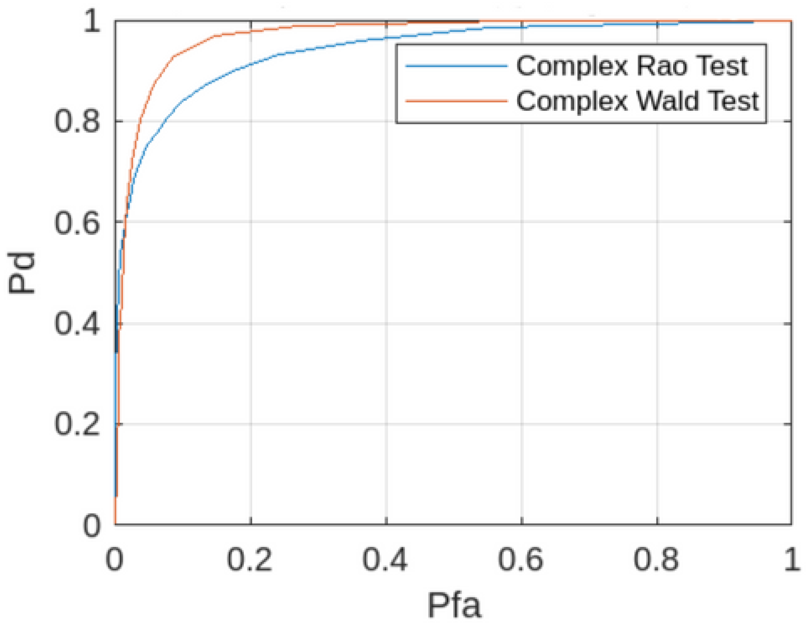
To evaluate the performance of the complex Rao and Wald tests for this example, we set $b_1=0.5+0.5j$ under the alternative hypothesis ${\mathcal{H}}_1$.

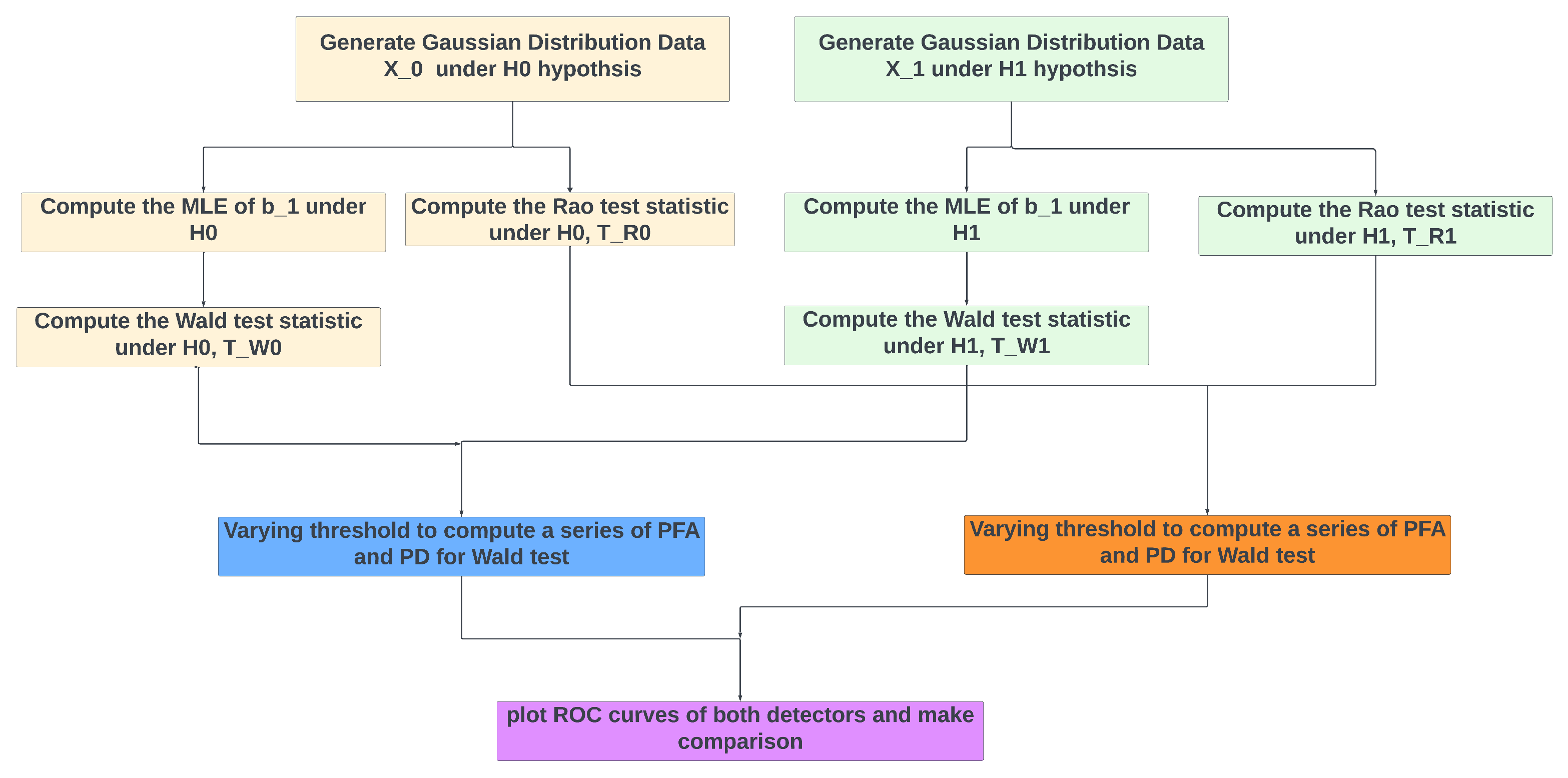
All simulations were conducted using Matlab by MathWorks, Inc.,(Portola Valley, CA, USA). The Receiver Operating Characteristic (ROC) curves, depicting the relationship between the Probability of Detection ($P_d$) and the Probability of False Alarm ($P_{fa}$), were generated to characterize the performance of the detectors. The construction of the ROC curve involved the following steps: for each simulation setup, a substantial number of Monte Carlo simulation trials were executed. The test statistics were computed under both scenarios, $H_1$ and $H_0$. Specifically, simulations were run 50,000 times, resulting in a vector of size 50,000 for the test statistic under $H_1$, denoted as $T_1$, and similarly, another vector of size 50,000 for the test statistic under $H_0$, denoted as $T_0$. Varying a threshold $\gamma$, any element in $T_0$ greater than $\gamma$ signified a false alarm trial, while any element in $T_1$ greater than $\gamma$ represented a correct detection trial. By systematically varying the threshold $\gamma$, a series of $(P_{fa},P_d)$ pairs were obtained, constituting the ROC curve. This curve, encapsulating the trade-off between $P_d$ and $P_{fa}$, was generated as a vector of such pairs by varying the threshold $\gamma$. Figure 1 presents a high-level flowchart outlining the steps involved in the Monte Carlo simulations for generating the ROC curves for both the Wald and Rao tests.

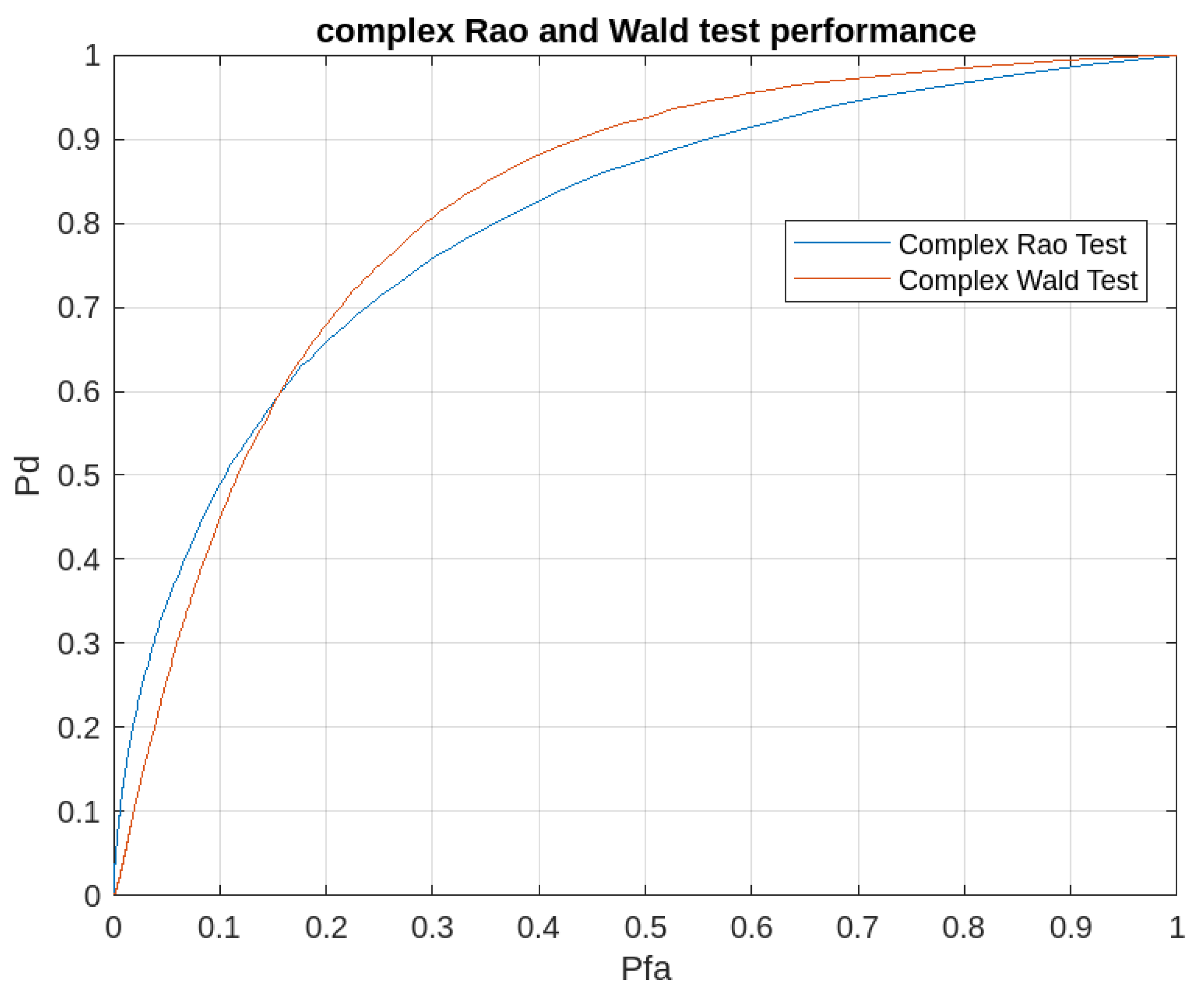
The ROC curves of the derived complex Rao and Wald test is given in Figure 2.

The results demonstrate that both the complex Rao and Wald tests exhibit commendable performance when confronted with limited data records. Notably, the complex Wald test outperforms the complex Rao test, aligning with expectations given that the latter generally demonstrates suboptimal performance. This performance disparity is expected considering that the complex Rao test, while less computationally intensive, as it does not necessitate the MLEs of the unknown parameters under ${\mathcal{H}}_1$, inherently delivers slightly inferior performance.

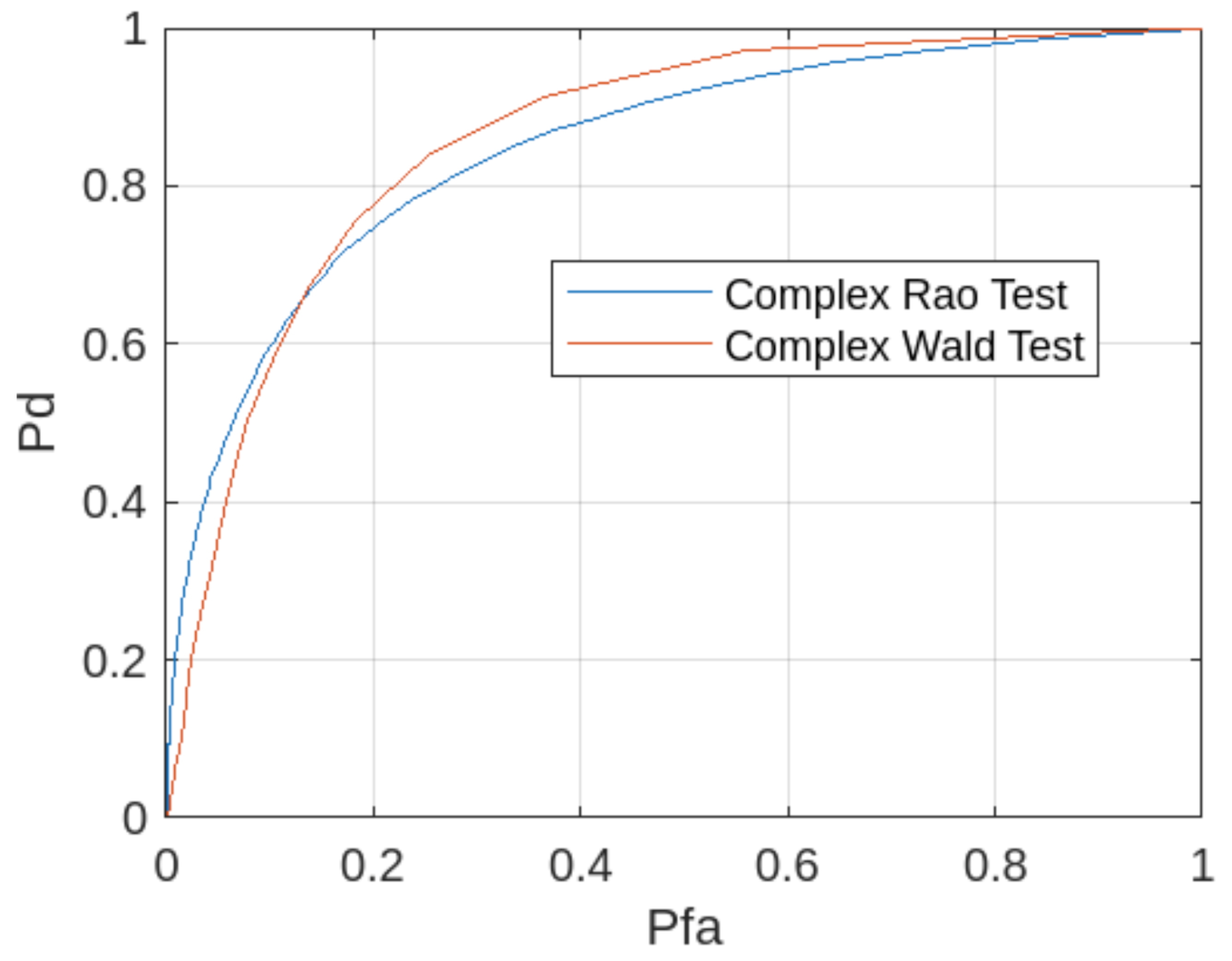
A second illustrative example is presented, where $b_1=0.3+0.3j$, representing a more challenging scenario compared to the earlier instance. Figure 3 showcases the performance of both proposed detectors in this setting. It is evident that in comparison to the prior example, the detectors’ performance declines due to the smaller magnitude of $b_1$. Notably, the complex Wald test exhibits a slight edge over the complex Rao test in this more challenging scenario.

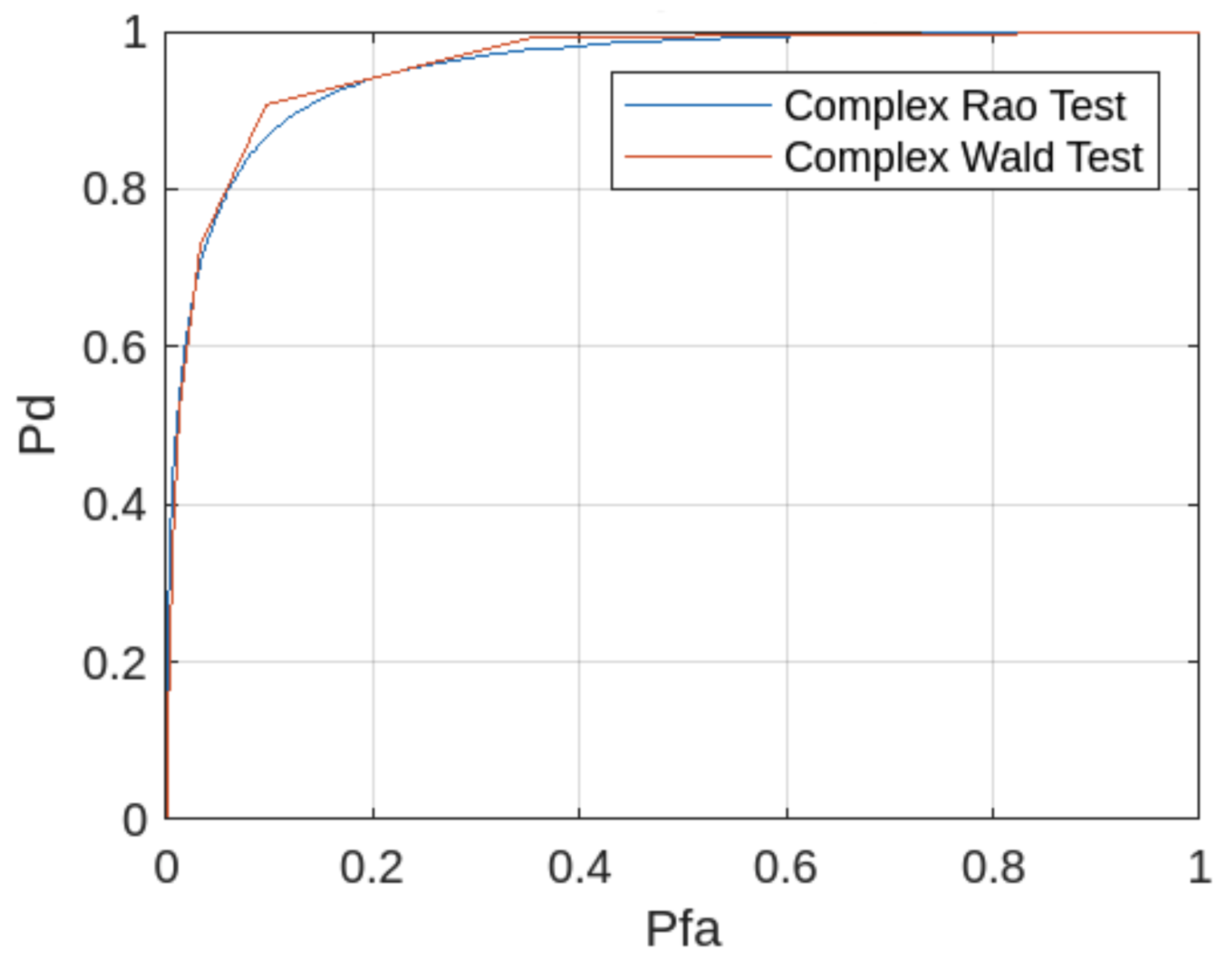
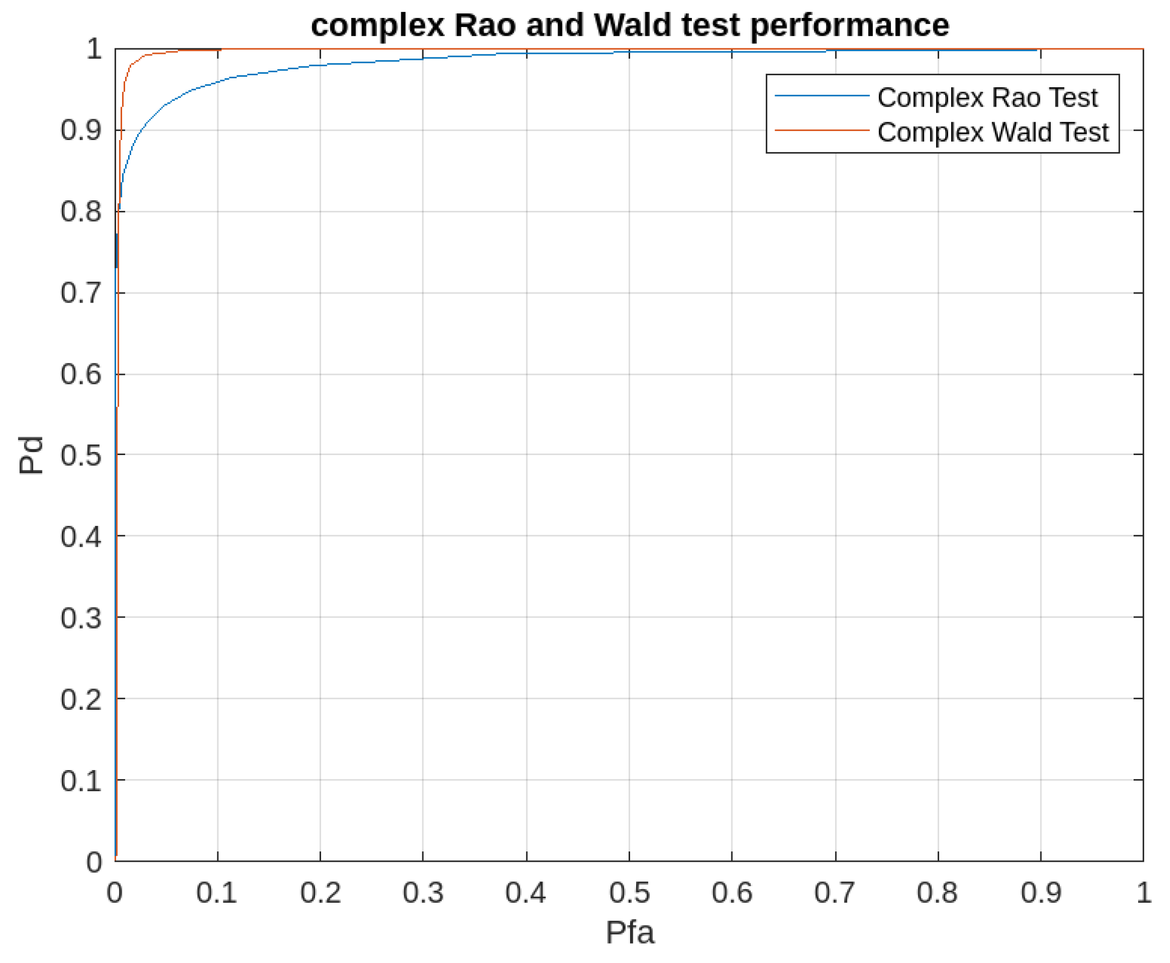
Next, we increase the number of IID samples from $N=4$ to $N=10$ and set the $b_1=0.3+0.3j$. The comparative performance of the two detectors is depicted in Figure 4. A comparative analysis with Figure 3 reveals a conspicuous enhancement in the performance of both detectors, attributable to the increased availability of data samples. Notably, it is discernible that in this scenario, the performance of the two detectors converges significantly, indicating that the Complex Rao and Wald tests exhibit asymptotic equivalence as the dataset size grows.

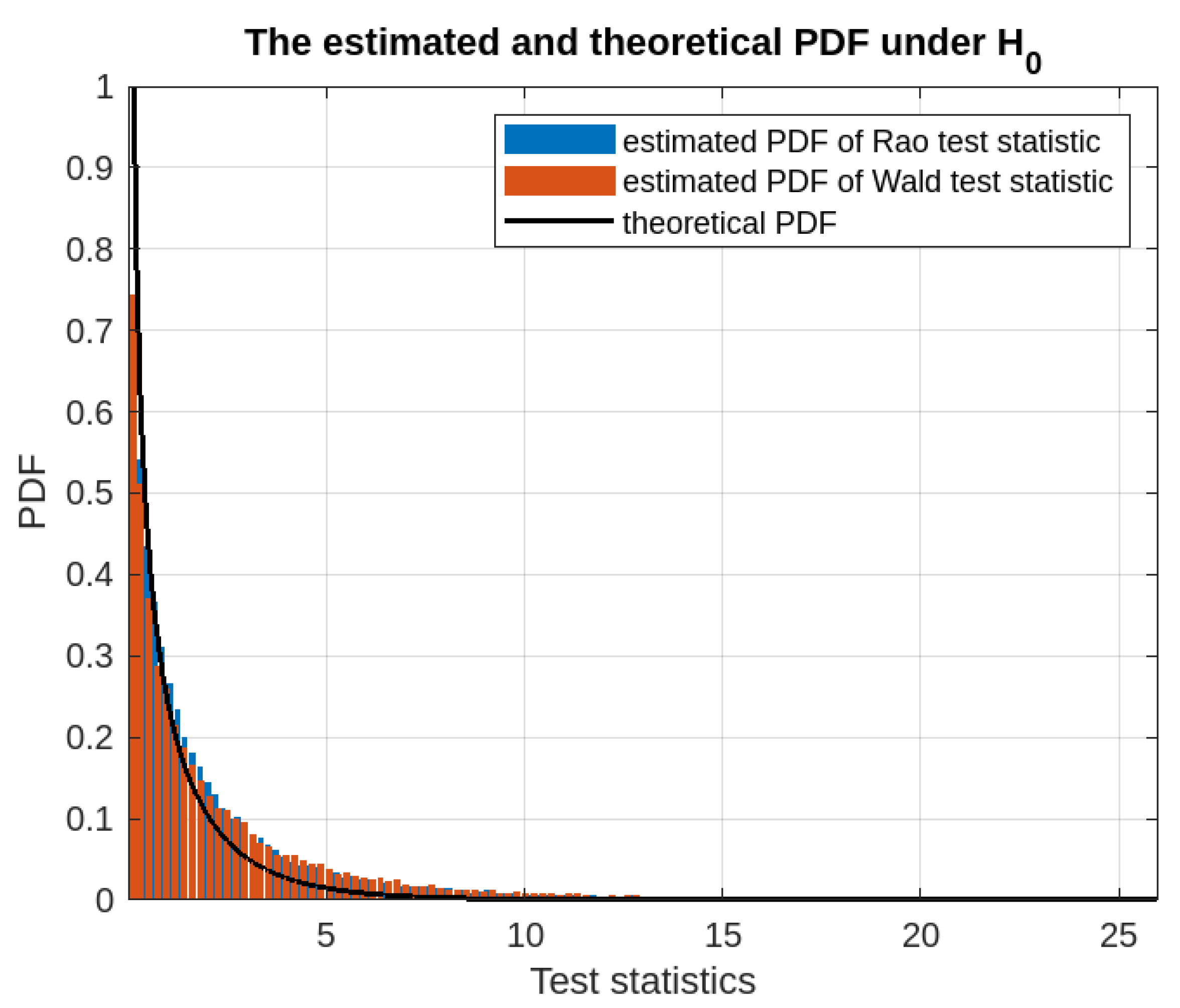
Both the Complex Rao test statistic and Complex Wald test under the null hypothesis ${\mathcal{H}}_0$ are chi-squared distributed with one degree of freedom, $T_R\left(\mathbf{X}\right)\sim {\chi }_1^2$ [28]. The performance of the Rao test and Wald test can be found asymptotically or as $N\to \infty$. Estimated probability density function (PDFs), shown as bar plots, for both the Rao test and the Wald test, and the theoretical asymptotic ${\chi }_1^2$ PDF are shown in Figure 5. Notably, even with a limited data record of $N=4$, the estimated PDFs remarkably align with the theoretical distribution.

The detectors’ performance is also dependent on the base matrix ${\mathbf{D}}_B$. Next, we double the magnitude of each element of ${\mathbf{D}}_B$; that is,

$${\mathbf{D}}_B=\left[\begin{array}{cccc}1.06& 0& 0& 0\\ -0.52+0.5j& 1.06& 0& 0\\ -0.24+0.2j& -0.66+0.56j& 1.02& 0\\ 0& -0.34-0.20j& 0.4-0.54j& 1.0\end{array}\right]$$

(50)

and keep the rest of the setup unchanged with $N=4$ and $b_1=0.5+0.5j$. The two detectors’ performances can be found in Figure 6.

In comparison with Figure 2, it is evident that both detectors’ performances have degraded due to the larger base matrix. Next, we show the detectors’ performance change when the base matrix become smaller. We half each element of ${\mathbf{D}}_B$; that is,

$${\mathbf{D}}_B=\left[\begin{array}{cccc}0.265& 0& 0& 0\\ -0.13+0.125j& 0.265& 0& 0\\ -0.06+0.05j& -0.165+0.14j& 0.255& 0\\ 0& -0.085-0.05j& 0.1-0.135j& 0.25\end{array}\right]$$

(51)

and keep the rest of the setup unchanged with $N=4$ and $b_1=0.5+0.5j$. The two detectors’ performances can be found in Figure 7. Compared with Figure 2, clearly both detectors’ performances have improved due to the smaller base matrix.

4.2. Equivalence among Complex Wald, Rao Test and GlRT for Linear Model

When the unknown parameter is present in the covariance matrix, the structure of the FIM does not attain the special form that allows one to use the Reduced Complex Wald Test and the Reduced Complex Rao Test [19]. One such case is the problem of testing the bandedness of the covariance matrix discussed above. As a counter example, in this section, we show the equivalence between the Complex Rao Test and the Complex Wald Test for an important case of general practical interest—the complex Gaussian linear model. A large number of signal processing, detection and estimation problems like radar signal processing and communications can be represented by a linear model, and hence it is of practical importance to discuss the topic.

4.2.1. Complex Classical Linear Model Testing Problem

First, we apply complex Wald test to the complex linear model problem. Assume the data are modeled according to [23]:

$$\tilde{\mathbf{x}}=\tilde{\mathbf{H}}\tilde{\mathit{\theta }}+\tilde{\mathbf{w}},$$

where $\tilde{\mathbf{H}}\in {\mathbb{C}}^{N\times p}$ is a known matrix with $N>p$ and full rank, $\tilde{\mathit{\theta }}$ is an unknown complex $p\times 1$ parameter vector, and $\tilde{\mathbf{w}}$ is a complex $N\times 1$ random vector with PDF $\tilde{\mathbf{w}}\sim \mathcal{CN}(\mathbf{0},\tilde{\mathbf{C}})$, with $\tilde{\mathbf{C}}\in {\mathbb{C}}^{N\times N}$. The testing problem is equivalent to deciding between two hypotheses:

$$\begin{array}{c}\hfill {\mathcal{H}}_0:\tilde{\mathit{\theta }}=\mathbf{0}\\ \hfill {\mathcal{H}}_1:\tilde{\mathit{\theta }}\ne \mathbf{0}\end{array}$$

Then, based on the properties of the complex Gaussian PDF

$$\tilde{\mathbf{x}}\sim \mathcal{CN}(\tilde{\mu },\tilde{\mathbf{C}})$$

so that $\tilde{\mu }=\tilde{\mathbf{H}}\tilde{\mathit{\theta }}$ and $\tilde{\mathbf{C}}\left(\tilde{\mathit{\theta }}\right)=\tilde{\mathbf{C}}$(not dependent on $\tilde{\mathit{\theta }}$ or ${\tilde{\mathit{\theta }}}^{*}$). The PDF is

$$p(\tilde{\mathbf{x}};\tilde{\mathit{\theta }})=\frac{1}{{\pi }^{N}det\left(\tilde{\mathbf{C}}\right)}exp[-{(\tilde{\mathbf{x}}-\tilde{\mathbf{H}}\tilde{\mathit{\theta }})}^H{\tilde{\mathbf{C}}}^{-1}(\tilde{\mathbf{x}}-\tilde{\mathbf{H}}\tilde{\mathit{\theta }})].$$

We have

$$\begin{array}{cc}\hfill \frac{\partial lnp(\tilde{\mathbf{x}};\tilde{\mathit{\theta }})}{\partial {\tilde{\mathit{\theta }}}^{*}}& =-\frac{\partial {(\tilde{\mathbf{x}}-\tilde{\mathbf{H}}\tilde{\mathit{\theta }})}^H{\tilde{\mathbf{C}}}^{-1}(\tilde{\mathbf{x}}-\tilde{\mathbf{H}}\tilde{\mathit{\theta }})}{\partial {\tilde{\mathit{\theta }}}^{*}}\hfill \\ & ={\tilde{\mathbf{H}}}^H{\tilde{\mathbf{C}}}^{-1}(\tilde{\mathbf{x}}-\tilde{\mathbf{H}}\tilde{\mathit{\theta }})\hfill \end{array}$$

Therefore, the MLE of $\tilde{\mathit{\theta }}$ under ${\mathcal{H}}_1$ is ${\widehat{\tilde{\mathit{\theta }}}}_1={\left({\tilde{\mathbf{H}}}^H{\tilde{\mathbf{C}}}^{-1}\tilde{\mathbf{H}}\right)}^{-1}{\tilde{\mathbf{H}}}^H{\tilde{\mathbf{C}}}^{-1}\tilde{\mathbf{x}}$. Also we have, as shown in [23],

$$\tilde{\mathbf{I}}\left(\tilde{\mathit{\theta }}\right)={\tilde{\mathbf{H}}}^H{\tilde{\mathbf{C}}}^{-1}\tilde{\mathbf{H}},$$

and the real FIM has the special form

$${\mathbf{I}}^{-1}\left(\mathit{\xi }\right)=\frac{1}{2}\left[\begin{array}{cc}\mathrm{Re}\{{\left({\tilde{\mathbf{H}}}^H{\tilde{\mathbf{C}}}^{-1}\tilde{\mathbf{H}}\right)}^{-1}\}& -Im\left\{{\left({\tilde{\mathbf{H}}}^H{\tilde{\mathbf{C}}}^{-1}\tilde{\mathbf{H}}\right)}^{-1}\right\}\\ Im\left\{{\left({\tilde{\mathbf{H}}}^H{\tilde{\mathbf{C}}}^{-1}\tilde{\mathbf{H}}\right)}^{-1}\right\}& \mathrm{Re}\{{\left({\tilde{\mathbf{H}}}^H{\tilde{\mathbf{C}}}^{-1}\tilde{\mathbf{H}}\right)}^{-1}\}\end{array}\right].$$

4.2.2. Generalized Likelihood Ratio Test (GlRT)

The GLRT decides ${\mathcal{H}}_1$ if

$$L_G\left(\tilde{\mathbf{x}}\right)=\frac{p(\tilde{\mathbf{x}};{\widehat{\tilde{\mathit{\theta }}}}_1)}{p(\tilde{\mathbf{x}};{\tilde{\mathit{\theta }}}_0=\mathbf{0})}>\gamma$$

(52)

We have

$$\begin{array}{ccc}\hfill 2ln{L}_G\left(\tilde{\mathbf{x}}\right)& =& 2ln\frac{p(\tilde{\mathbf{x}};{\widehat{\tilde{\mathit{\theta }}}}_1)}{p(\tilde{\mathbf{x}};{\tilde{\mathit{\theta }}}_0=\mathbf{0})}\hfill \\ & =& 2\left({\tilde{\mathbf{x}}}^H{\tilde{\mathbf{C}}}^{-1}\tilde{\mathbf{x}}-{(\tilde{\mathbf{x}}-\tilde{\mathbf{H}}{\widehat{\tilde{\mathit{\theta }}}}_1)}^H{\tilde{\mathbf{C}}}^{-1}(\tilde{\mathbf{x}}-\tilde{\mathbf{H}}{\widehat{\tilde{\mathit{\theta }}}}_1)\right)\hfill \\ & =& 2({\tilde{\mathbf{x}}}^H{\tilde{\mathbf{C}}}^{-1}\tilde{\mathbf{x}}-{\tilde{\mathbf{x}}}^H{\tilde{\mathbf{C}}}^{-1}\tilde{\mathbf{x}}\hfill \\ & & +{\tilde{\mathbf{x}}}^H{\tilde{\mathbf{C}}}^{-1}\tilde{\mathbf{H}}{\left({\tilde{\mathbf{H}}}^H{\tilde{\mathbf{C}}}^{-1}\tilde{\mathbf{H}}\right)}^{-1}{\tilde{\mathbf{H}}}^H{\tilde{\mathbf{C}}}^{-1}\tilde{\mathbf{x}}\hfill \\ & & +{\tilde{\mathbf{x}}}^H{\tilde{\mathbf{C}}}^{-1}\tilde{\mathbf{H}}{\left({\tilde{\mathbf{H}}}^H{\tilde{\mathbf{C}}}^{-1}\tilde{\mathbf{H}}\right)}^{-1}{\tilde{\mathbf{H}}}^H{\tilde{\mathbf{C}}}^{-1}\tilde{\mathbf{x}}\hfill \\ & & -{\tilde{\mathbf{x}}}^H{\tilde{\mathbf{C}}}^{-1}\tilde{\mathbf{H}}{\left({\tilde{\mathbf{H}}}^H{\tilde{\mathbf{C}}}^{-1}\tilde{\mathbf{H}}\right)}^{-1}{\tilde{\mathbf{H}}}^H{\tilde{\mathbf{C}}}^{-1}\tilde{\mathbf{H}}{\left({\tilde{\mathbf{H}}}^H{\tilde{\mathbf{C}}}^{-1}\tilde{\mathbf{H}}\right)}^{-1}{\tilde{\mathbf{H}}}^H{\tilde{\mathbf{C}}}^{-1}\tilde{\mathbf{x}})\hfill \\ & =& 2{\tilde{\mathbf{x}}}^H{\tilde{\mathbf{C}}}^{-1}\tilde{\mathbf{H}}{\left({\tilde{\mathbf{H}}}^H{\tilde{\mathbf{C}}}^{-1}\tilde{\mathbf{H}}\right)}^{-1}{\tilde{\mathbf{H}}}^H{\tilde{\mathbf{C}}}^{-1}\tilde{\mathbf{x}}\hfill \end{array}$$

(53)

4.2.3. Complex Rao Test

The complex Rao test is [19]

$$\begin{array}{ccc}\hfill T_{\tilde{R}}\left(\tilde{\mathbf{x}}\right)& =& 2{\frac{\partial ln{p}_{\tilde{\mathbf{x}}}(\tilde{\mathbf{x}};\tilde{\mathit{\theta }})}{\partial {\tilde{\mathit{\theta }}}^{*}}}^H{\tilde{\mathbf{I}}}^{-1}\left(\tilde{\mathit{\theta }}\right)\frac{\partial ln{p}_{\tilde{\mathbf{x}}}(\tilde{\mathbf{x}};\tilde{\mathit{\theta }})}{\partial {\tilde{\mathit{\theta }}}^{*}}{|}_{\tilde{\mathit{\theta }}={\tilde{\mathit{\theta }}}_0}\hfill \\ & =& 2{\left[{\tilde{\mathbf{H}}}^H{\tilde{\mathbf{C}}}^{-1}(\tilde{\mathbf{x}}-\tilde{\mathbf{H}}\tilde{\mathit{\theta }})\right]}^H{\left({\tilde{\mathbf{H}}}^H{\tilde{\mathbf{C}}}^{-1}\tilde{\mathbf{H}}\right)}^{-1}\left[{\tilde{\mathbf{H}}}^H{\tilde{\mathbf{C}}}^{-1}(\tilde{\mathbf{x}}-\tilde{\mathbf{H}}\tilde{\mathit{\theta }})\right]{|}_{\tilde{\mathit{\theta }}=\mathbf{0}}\hfill \\ & =& 2{\tilde{\mathbf{x}}}^H{\tilde{\mathbf{C}}}^{-1}\tilde{\mathbf{H}}{\left({\tilde{\mathbf{H}}}^H{\tilde{\mathbf{C}}}^{-1}\tilde{\mathbf{H}}\right)}^{-1}{\tilde{\mathbf{H}}}^H{\tilde{\mathbf{C}}}^{-1}\tilde{\mathbf{x}}\hfill \end{array}$$

(54)

4.2.4. Complex Wald Test

The real FIM of this problem has a special form, so Theorem 2 applies. The complex Wald test is

$$\begin{array}{ccc}\hfill T_{\tilde{W}}\left(\tilde{\mathbf{x}}\right)& =& 2{(\tilde{\mathit{\theta }}-{\tilde{\mathit{\theta }}}_0)}^H\tilde{\mathbf{I}}\left(\tilde{\mathit{\theta }}\right)(\tilde{\mathit{\theta }}-{\tilde{\mathit{\theta }}}_0){|}_{\tilde{\mathit{\theta }}={\widehat{\tilde{\mathit{\theta }}}}_1}\hfill \\ & =& 2{\left[{\left({\tilde{\mathbf{H}}}^H{\tilde{\mathbf{C}}}^{-1}\tilde{\mathbf{H}}\right)}^{-1}{\tilde{\mathbf{H}}}^H{\tilde{\mathbf{C}}}^{-1}\tilde{\mathbf{x}}\right]}^H\left({\tilde{\mathbf{H}}}^H{\tilde{\mathbf{C}}}^{-1}\tilde{\mathbf{H}}\right){\left({\tilde{\mathbf{H}}}^H{\tilde{\mathbf{C}}}^{-1}\tilde{\mathbf{H}}\right)}^{-1}{\tilde{\mathbf{H}}}^H{\tilde{\mathbf{C}}}^{-1}\tilde{\mathbf{x}}\hfill \\ & =& 2{\tilde{\mathbf{x}}}^H{\tilde{\mathbf{C}}}^{-1}\tilde{\mathbf{H}}{\left({\tilde{\mathbf{H}}}^H{\tilde{\mathbf{C}}}^{-1}\tilde{\mathbf{H}}\right)}^{-1}{\tilde{\mathbf{H}}}^H{\tilde{\mathbf{C}}}^{-1}\tilde{\mathbf{x}}\hfill \end{array}$$

(55)

Compared with the results obtained by using GLRT and the complex Rao Test for the same problem, all three detectors are equivalent in this case. Next, we show the root cause of this equivalence.

4.2.5. The Root Cause of the Equivalence

First,

$$\frac{\partial ln{p}_{\tilde{\mathbf{x}}}(\tilde{\mathbf{x}};\tilde{\mathit{\theta }})}{\partial {\tilde{\mathit{\theta }}}^{*}}=\tilde{\mathbf{I}}\left(\tilde{\mathit{\theta }}\right)(\widehat{\tilde{\mathit{\theta }}}-\tilde{\mathit{\theta }})$$

(56)

where $\tilde{\mathit{\theta }}$ is the true value. Because the complex FIM is not dependent on the true value of the unknown parameters, $\tilde{\mathbf{I}}\left(\tilde{\mathit{\theta }}\right)=\tilde{\mathbf{I}}\left({\widehat{\tilde{\mathit{\theta }}}}_1\right)$, we have

$$\frac{\partial ln{p}_{\tilde{\mathbf{x}}}(\tilde{\mathbf{x}};\tilde{\mathit{\theta }})}{\partial {\tilde{\mathit{\theta }}}^{*}}=\tilde{\mathbf{I}}\left({\widehat{\tilde{\mathit{\theta }}}}_1\right)(\widehat{\tilde{\mathit{\theta }}}-\tilde{\mathit{\theta }})$$

(57)

So, by integrating with respect to ${\tilde{\mathit{\theta }}}^{*}$, it produces

$$ln{p}_{\tilde{\mathbf{x}}}(\tilde{\mathbf{x}};\tilde{\mathit{\theta }})=-{(\widehat{\tilde{\mathit{\theta }}}-\tilde{\mathit{\theta }})}^H\tilde{\mathbf{I}}\left(\widehat{\tilde{\mathit{\theta }}}\right)(\widehat{\tilde{\mathit{\theta }}}-\tilde{\mathit{\theta }})+c\left(\widehat{\tilde{\mathit{\theta }}}\right)$$

(58)

since the constant of integration must be $c\left(\widehat{\tilde{\mathit{\theta }}}\right)=ln{p}_{\tilde{\mathbf{x}}}(\tilde{\mathbf{x}};\widehat{\tilde{\mathit{\theta }}})$.

The GLRT becomes

$$L_G\left(\tilde{\mathbf{x}}\right)=\frac{p(\tilde{\mathbf{x}};{\widehat{\tilde{\mathit{\theta }}}}_1)}{p(\tilde{\mathbf{x}};{\tilde{\mathit{\theta }}}_0)}=\frac{p(\tilde{\mathbf{x}};{\widehat{\tilde{\mathit{\theta }}}}_1)}{p(\tilde{\mathbf{x}};{\widehat{\tilde{\mathit{\theta }}}}_1)exp\left[-{({\widehat{\tilde{\mathit{\theta }}}}_1-{\tilde{\mathit{\theta }}}_0)}^H\tilde{\mathbf{I}}\left({\widehat{\tilde{\mathit{\theta }}}}_1\right)({\widehat{\tilde{\mathit{\theta }}}}_1-{\tilde{\mathit{\theta }}}_0)\right]}$$

(59)

Thus,

$$2ln{L}_G\left(\tilde{\mathbf{x}}\right)=2{({\widehat{\tilde{\mathit{\theta }}}}_1-{\tilde{\mathit{\theta }}}_0)}^H\tilde{\mathbf{I}}\left({\widehat{\tilde{\mathit{\theta }}}}_1\right)({\widehat{\tilde{\mathit{\theta }}}}_1-{\tilde{\mathit{\theta }}}_0)$$

(60)

This explains why the GLRT and the complex Wald test coincide for the complex linear model. Furthermore, to establish the equivalence between the complex Rao test and the Generalized Likelihood Ratio Test (GLRT), we use Equation (56)

$$(\widehat{\tilde{\mathit{\theta }}}-\tilde{\mathit{\theta }})={\tilde{\mathbf{I}}}^{-1}\left(\tilde{\mathit{\theta }}\right)\frac{\partial ln{p}_{\tilde{\mathbf{x}}}(\tilde{\mathbf{x}};\tilde{\mathit{\theta }})}{\partial {\tilde{\mathit{\theta }}}^{*}}$$

(61)

Specially,

$$({\widehat{\tilde{\mathit{\theta }}}}_1-{\tilde{\mathit{\theta }}}_0)={\tilde{\mathbf{I}}}^{-1}\left({\tilde{\mathit{\theta }}}_0\right)\frac{\partial ln{p}_{\tilde{\mathbf{x}}}(\tilde{\mathbf{x}};\tilde{\mathit{\theta }})}{\partial {\tilde{\mathit{\theta }}}^{*}}{|}_{\tilde{\mathit{\theta }}={\tilde{\mathit{\theta }}}_0}$$

(62)

By substituting (62) to (60), we have

$$\begin{array}{c}\hfill \begin{array}{cc}\hfill 2ln{L}_G\left(\tilde{\mathbf{x}}\right)& =2{\left({\tilde{\mathbf{I}}}^{-1}\left({\tilde{\mathit{\theta }}}_0\right)\frac{\partial ln{p}_{\tilde{\mathbf{x}}}(\tilde{\mathbf{x}};\tilde{\mathit{\theta }})}{\partial {\tilde{\mathit{\theta }}}^{*}}{|}_{\tilde{\mathit{\theta }}={\tilde{\mathit{\theta }}}_0}\right)}^H\tilde{\mathbf{I}}\left({\widehat{\tilde{\mathit{\theta }}}}_1\right)\left({\tilde{\mathbf{I}}}^{-1}\left({\tilde{\mathit{\theta }}}_0\right)\frac{\partial ln{p}_{\tilde{\mathbf{x}}}(\tilde{\mathbf{x}};\tilde{\mathit{\theta }})}{\partial {\tilde{\mathit{\theta }}}^{*}}{|}_{\tilde{\mathit{\theta }}={\tilde{\mathit{\theta }}}_0}\right)\hfill \\ & =2\frac{\partial ln{p}_{\tilde{\mathbf{x}}}(\tilde{\mathbf{x}};\tilde{\mathit{\theta }})}{\partial {\tilde{\mathit{\theta }}}^{*}}{|}_{\tilde{\mathit{\theta }}={\tilde{\mathit{\theta }}}_0}^H{\tilde{\mathbf{I}}}^{-1}\left({\tilde{\mathit{\theta }}}_0\right)\tilde{\mathbf{I}}\left({\widehat{\tilde{\mathit{\theta }}}}_1\right){\tilde{\mathbf{I}}}^{-1}\left({\tilde{\mathit{\theta }}}_0\right)\frac{\partial ln{p}_{\tilde{\mathbf{x}}}(\tilde{\mathbf{x}};\tilde{\mathit{\theta }})}{\partial {\tilde{\mathit{\theta }}}^{*}}{|}_{\tilde{\mathit{\theta }}={\tilde{\mathit{\theta }}}_0}\hfill \\ & =2\frac{\partial ln{p}_{\tilde{\mathbf{x}}}(\tilde{\mathbf{x}};\tilde{\mathit{\theta }})}{\partial {\tilde{\mathit{\theta }}}^{*}}{|}_{\tilde{\mathit{\theta }}={\tilde{\mathit{\theta }}}_0}^H{\tilde{\mathbf{I}}}^{-1}\left({\tilde{\mathit{\theta }}}_0\right)\frac{\partial ln{p}_{\tilde{\mathbf{x}}}(\tilde{\mathbf{x}};\tilde{\mathit{\theta }})}{\partial {\tilde{\mathit{\theta }}}^{*}}{|}_{\tilde{\mathit{\theta }}={\tilde{\mathit{\theta }}}_0}\hfill \end{array}\end{array}$$

(63)

where we have used the property of $\tilde{\mathbf{I}}\left(\tilde{\mathit{\theta }}\right)=\tilde{\mathbf{I}}\left({\tilde{\mathit{\theta }}}_0\right)=\tilde{\mathbf{I}}\left({\widehat{\tilde{\mathit{\theta }}}}_1\right)$. This completes the proof that the complex Rao test and the GLRT are equivalent for the complex linear model. Consequently, it also proves the equivalence among the aforementioned three detectors for the complex linear model. In summary, the equivalence stems from the fact that the complex FIM of the linear model $\tilde{\mathbf{I}}\left(\tilde{\mathit{\theta }}\right)={\tilde{\mathbf{H}}}^H{\tilde{\mathbf{C}}}^{-1}\tilde{\mathbf{H}}$ does not depend on the true value of $\tilde{\mathit{\theta }}$. In particular, we have $\tilde{\mathbf{I}}\left(\tilde{\mathit{\theta }}\right)=\tilde{\mathbf{I}}\left({\tilde{\mathit{\theta }}}_0\right)=\tilde{\mathbf{I}}\left({\widehat{\tilde{\mathit{\theta }}}}_1\right)$, and hence the complex Rao test and Wald test are both equivalent to the GLRT without extra constraints.

5. Conclusions

The utilization of banding techniques has gained prominence in the estimation of covariance matrices, particularly in scenarios with limited sample sizes within high-dimensional signal processing. Before adopting such techniques, assessing the matrix’s ‘bandability’ becomes crucial. To this end, we have derived both the complex Rao test and the complex Wald test, specifically tailored for evaluating the bandedness of the Cholesky factor matrix within the inverse of the covariance matrix. The computational cost of the Rao test is comparatively lower, while implementing the complex Wald test demands obtaining maximum likelihood estimates under the alternative hypothesis. Consequently, the latter proofs more challenging to derive and incur higher computational expenses. We present examples and simulations to assess the performance of these proposed detectors. In our evaluations, the Wald test exhibits slightly superior performance in cases with smaller ‘signal’ magnitudes and significantly outperforms the complex parameter Rao test as the tested parameter grows larger. However, as the sample size increases, the performance gap between the two detectors diminishes. Notably, both detectors demonstrate asymptotic optimality with a substantial volume of available data.These derived detectors can serve as a preparatory step before implementing banding techniques for covariance matrix estimation. Furthermore, they extend applicability beyond bandedness assessment by enabling tests for zero elements within a matrix, achieved by appropriately modifying the basis matrix ${\mathbf{\Phi }}_k$. Moreover, our investigation reveals the equivalence between the complex Rao test, Wald test, and GLRT within the general complex Gaussian linear model, shedding light on the underlying mechanisms of this equivalence. In our forthcoming research, we aim to delve deeper into the computational costs associated with these two detectors.

References

- Melvin, W.L. A STAP Overview. IEEE AES Syst. Mag.—Spec. Tutor. Issue 2004, 19, 19–35. [Google Scholar] [CrossRef]
- Anderson, T. An Introduction to Multivariate Statistical Analysis, 3rd ed.; Wiley: Hoboken, NJ, USA, 2003. [Google Scholar]
- Melvin, W.L.; Showman, G.A. An Approach to Knowledge-Aided Covariance Estimation. IEEE Trans. Aerosp. Electron. Syst. 2006, 42, 1021–1042. [Google Scholar] [CrossRef]
- Bickel, P.J.; Levina, E. Covariance regularization by thresholding. Ann. Statist. 2008, 36, 2577–2604. [Google Scholar] [CrossRef] [PubMed]
- Rothman, A.; Levina, L.; Zhu, J. Generalized thresholding of large covariance matrices. J. Am. Statist. Assoc. 2009, 104, 177–186. [Google Scholar] [CrossRef]
- Bickel, P.J.; Levina, E. Regularized estimation of large covariance matrices. Ann. Statist. 2008, 36, 199–227. [Google Scholar] [CrossRef]
- Cai, T.T.; Zhang, C.; Zhou, H. Optimal rates of convergence for covariance matrix estimation. Ann. Statist. 2010, 38, 2118–2144. [Google Scholar] [CrossRef]
- Rothman, A.; Levina, L.; Zhu, J. A new approach to Cholesky-based covariance regularization in high dimensions. Biometrika 2010, 97, 539–550. [Google Scholar] [CrossRef]
- An, B.; Guo, J.; Liu, Y. Hypothesis testing for band size detection of high-dimensional banded precision matrices. Biometrika 2014, 101, 477–483. [Google Scholar] [CrossRef]
- Wu, W.B.; Pourahmadi, M. Nonparametric estimation of large covariance matrices of longitudinal data. Biometrika 2003, 90, 831–844. [Google Scholar] [CrossRef]
- Qian, F.; Zhang, W.; Chen, Y. Adaptive banding covariance estimation for high-dimensional multivariate longitudinal data. Can. J. Stat. 2021, 49, 906–938. [Google Scholar] [CrossRef]
- Wiesel, A.; Bibi, O.; Globerson, A. Time varying autoregressive moving average models for covariance estimation. IEEE Trans. Signal Process. 2013, 61, 2791–2801. [Google Scholar] [CrossRef]
- Zhu, Z.; Kay, S. On Bayesian Exponentially Embedded Family for model order selection. IEEE Trans. Signal Process. 2018, 66, 933–943. [Google Scholar] [CrossRef]
- Qiu, Y.-M.; Chen, S.X. Test for bandedness of high dimensional covariance matrices with bandwidth estimation. Ann. Stat. 2002, 40, 1285–1314. [Google Scholar] [CrossRef]
- Peng, L.; Chen, S.X.; Zhou, W. More powerful tests for sparse high-dimensional covariances matrices. J. Multivar. Anal. 2016, 149, 124–143. [Google Scholar] [CrossRef]
- Zhu, Z.; Kay, S.; Raghavan, R.S. Information-theoretic optimal radar waveform design. IEEE Signal Process. Lett. 2017, 24, 274–278. [Google Scholar] [CrossRef]
- Schreier, P.J.; Scharf, L.L. Statistical Signal Processing of Complex-Valued Data: The Theory of Improper and Noncircular Signals; Cambridge University Press: Cambridge, UK, 2010. [Google Scholar]
- Adali, T.; Schreier, P.J.; Scharf, L.L. Complex-valued signal processing: The proper way to deal with impropriety. IEEE Trans. Signal Process. 2011, 59, 5101–5125. [Google Scholar] [CrossRef]
- Kay, S.; Zhu, Z. The complex parameter Rao test. IEEE Trans. Signal Process. 2016, 94, 6580–6588. [Google Scholar] [CrossRef]
- Sun, M.; Liu, W.; Liu, J.; Hao, C. Complex parameter Rao, Wald, Gradient, and Durbin Tests for multichannel signal detection. IEEE Trans. Signal Process. 2021, 70, 117–131. [Google Scholar] [CrossRef]
- Liu, W.; Xie, W.; Wang, Y. Rao and Wald tests for distributed targets detection with unknown signal steering. IEEE Signal Process. Lett. 2013, 20, 1086–1089. [Google Scholar]
- De Maio, A.; Iommelli, S. Coincidence of the Rao Test, Wald Test, and GLRT in partially homogeneous environment. IEEE Signal Process. Lett. 2008, 15, 385–388. [Google Scholar] [CrossRef]
- Kay, S. Fundamentals of Statistical Signal Processing: Estimation Theory; Prentice-Hall: Englewood Cliffs, NJ, USA, 1993. [Google Scholar]
- Liu, W.; Wang, Y.; Xie, W. Fisher information matrix, Rao test, and Wald test for complex-valued signals and their applications. Signal Process. 2014, 94, 1–5. [Google Scholar] [CrossRef]
- Zhu, Z.; Kay, S.; Cogun, F.; Raghavan, R.S. On detection of nonstationarity in radar signal processing. In Proceedings of the 2016 IEEE Radar Conference (RadarConf), Philadelphia, PA, USA, 2–6 May 2016; pp. 1–4. [Google Scholar]
- Zhu, Z.; Kay, S. The Rao test for testing handedness of complex-valued covariance matrix. In Proceedings of the 2016 IEEE International Conference on Acoustics, Speech and Signal Processing (ICASSP), Shanghai, China, 20–25 March 2016; pp. 3960–3963. [Google Scholar]
- Huang, B.; Basit, A.; Wang, W.; Zhang, S. Adaptive detection with Bayesian framework for FDA-MIMO radar. IEEE Geosci. Remote Sens. Lett. 2021, 19, 3509505. [Google Scholar] [CrossRef]
- Kay, S. Fundamentals of Statistical Signal Processing: Detection Theory; Prentice-Hall: Englewood Cliffs, NJ, USA, 1998. [Google Scholar]
Figure 1.
Illustration of Monte Carlo Simulation Steps for each simulation setup.
Figure 2.
ROC curve of the complex Rao and Wald test detector with .
Figure 3.
Figure 4.
ROC curve of the complex Rao and Wald test detector with and .
Figure 5.
Estimated and theoretical PDFs of the test statistic for N = 4.
Figure 6.
Complex Rao and Wald test performance with “larger” .
Figure 7.
Complex Rao and Wald test performance with “smaller” .
Disclaimer/Publisher’s Note: The statements, opinions and data contained in all publications are solely those of the individual author(s) and contributor(s) and not of MDPI and/or the editor(s). MDPI and/or the editor(s) disclaim responsibility for any injury to people or property resulting from any ideas, methods, instructions or products referred to in the content. |
© 2024 by the author. Licensee MDPI, Basel, Switzerland. This article is an open access article distributed under the terms and conditions of the Creative Commons Attribution (CC BY) license (https://creativecommons.org/licenses/by/4.0/).
Share and Cite
MDPI and ACS Style
Zhu, Z. Complex Parameter Rao and Wald Tests for Assessing the Bandedness of a Complex-Valued Covariance Matrix. Signals 2024, 5, 1-17. https://doi.org/10.3390/signals5010001
AMA Style
Zhu Z. Complex Parameter Rao and Wald Tests for Assessing the Bandedness of a Complex-Valued Covariance Matrix. Signals. 2024; 5(1):1-17. https://doi.org/10.3390/signals5010001
Chicago/Turabian StyleZhu, Zhenghan. 2024. "Complex Parameter Rao and Wald Tests for Assessing the Bandedness of a Complex-Valued Covariance Matrix" Signals 5, no. 1: 1-17. https://doi.org/10.3390/signals5010001