

Benford’s Law and Perceptual Features for Face Image Quality Assessment

Ronin Institute, Montclair, NJ 07043, USA
Signals 2023, 4(4), 859-876; https://doi.org/10.3390/signals4040047
Submission received: 18 August 2023
/
Revised: 14 September 2023
/
Accepted: 27 November 2023
/
Published: 5 December 2023
(This article belongs to the Special Issue The 2022 7th International Conference on Intelligent Information Processing)
Abstract
:The rapid growth in multimedia, storage systems, and digital computers has resulted in huge repositories of multimedia content and large image datasets in recent years. For instance, biometric databases, which can be used to identify individuals based on fingerprints, facial features, or iris patterns, have gained a lot of attention both from academia and industry. Specifically, face image quality assessment (FIQA) has become a very important part of face recognition systems, since the performance of such systems strongly depends on the quality of input data, such as blur, focus, compression, pose, or illumination. The main contribution of this paper is an analysis of Benford’s law-inspired first digit distribution and perceptual features for FIQA. To be more specific, I investigate the first digit distributions in different domains, such as wavelet or singular values, as quality-aware features for FIQA. My analysis revealed that first digit distributions with perceptual features are able to reach a high performance in the task of FIQA.
1. Introduction
Face image quality assessment (FIQA) is a field of research that focuses on evaluating the quality of face digital images. The goal of FIQA is to develop objective measures or algorithms that can assess the visual quality of face images, taking into account factors such as resolution, sharpness, noise, illumination, occlusions, and other image degradations. The importance of FIQA arises from its various practical applications. Accurate and reliable face image quality assessment is crucial in several domains, including biometrics, surveillance systems, facial recognition, identity verification, and image forensics. By determining the quality of face images, FIQA techniques help improve the performance and reliability of these systems by selecting or rejecting images based on their quality. Current approaches in face image quality assessment involve both subjective and objective methods [1]:
- 1.
- Subjective assessment: In this approach, human observers are involved in rating or scoring the quality of face images. These subjective ratings are collected through controlled experiments, where observers evaluate images based on specific quality attributes. The collected ratings are then used to create subjective quality databases or models.
- 2.
- Objective assessment: These methods aim to automate the process by developing computational algorithms that can predict image quality without human involvement. These methods utilize various features and metrics extracted from face images to quantify their quality. Some commonly used features include sharpness, contrast, noise, blur, and distortion. Machine learning techniques, such as regression or classification models, are often employed to train algorithms using annotated datasets [2].
- 3.
- Hybrid approaches: These methods combine subjective and objective methods to enhance the accuracy and reliability of face image quality assessment. These approaches leverage both human ratings and computational metrics to create more robust quality models. Machine learning algorithms can be trained using subjective ratings as the ground truth, allowing them to learn from human perception.
Recent advancements in deep learning have also impacted the field of FIQA. Convolutional neural networks (CNNs) have been employed to automatically learn features and classify face images based on their quality [3]. Overall, the goal of face image quality assessment is to provide reliable measures or algorithms that can assess the visual quality of face images objectively, enabling an improved performance and reliability in applications such as biometrics [4], surveillance [5], and facial recognition systems [6,7]. Face image quality assessment has also gained importance as a critical component of smart home and smart city applications that rely on facial recognition technology. Namely, it enhances security, access control, public safety, user experience, data accuracy, ethical considerations, and resource efficiency [8,9].
The goal of this study is to give a detailed analysis about the performance of Benford’s law-inspired and perceptual features in FIQA. The contributions of this study are as follows:
- 1.
- First, I investigate the first digit distributions (FDDs) of different image domains for FIQA.
- 2.
- Second, I empirically corroborate that the FDD of an image domain is a rather mediocre predictor for face image quality. However, taking the fusion of different domains’ FDDs results in a strong predictor whose performance can be further increased by considering several simple perceptual features, such as colorfulness, the global contrast factor, the dark channel feature, entropy, and phase congruency.
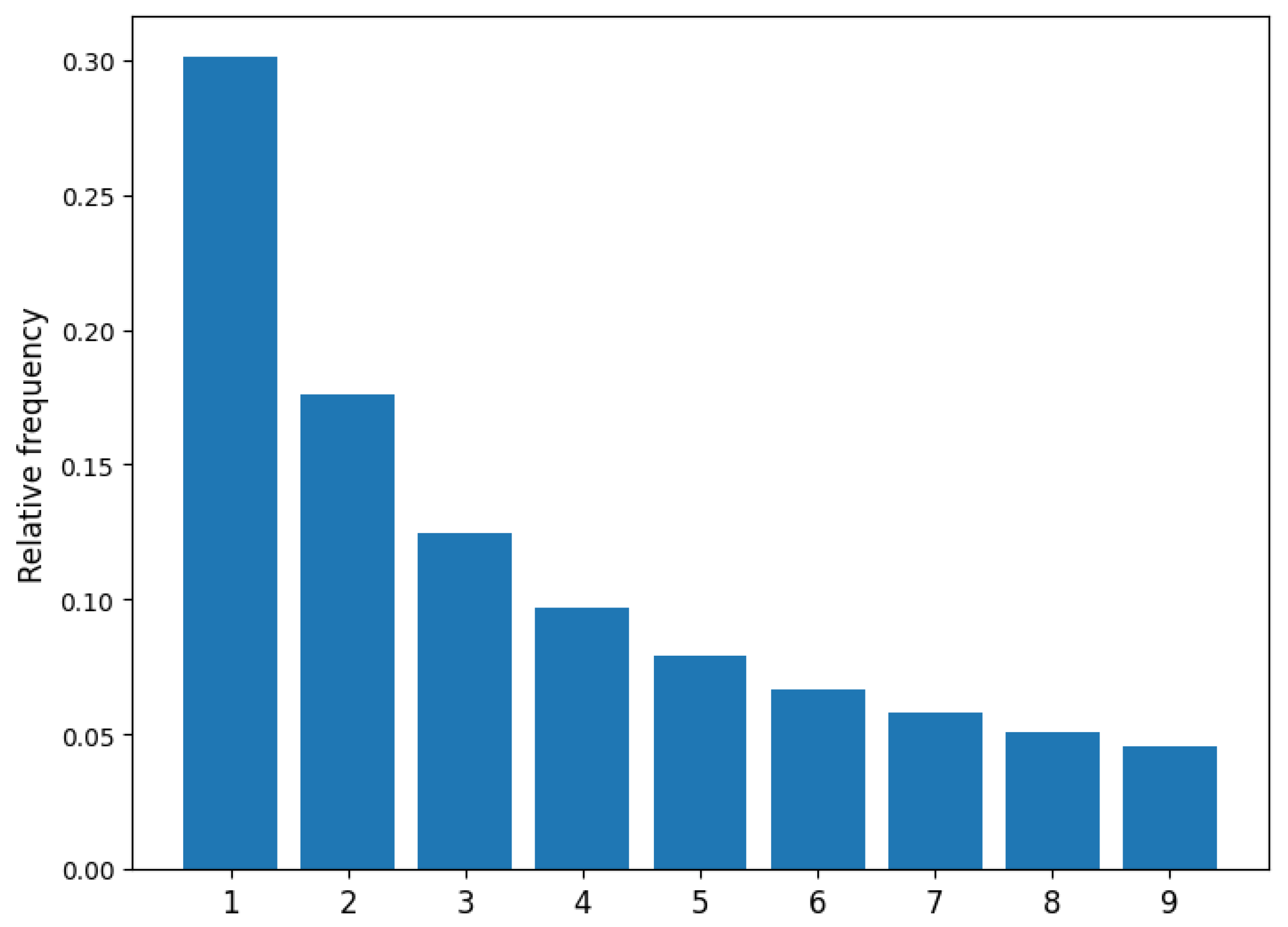
Benford’s law, also known in the literature as the law of anomalous numbers or first digit law, refers to an empirical observation that describes the frequency of leading digits in many numerical datasets, such as population numbers [10], geographical data [11], or physical constants [12]. Namely, the leading digits are not uniformly distributed but follow a pattern, which can be given as
where denotes the leading digit and is its relative frequency in a numerical dataset. The distribution defined by Equation (1) is depicted in Figure 1.
The remaining sections of this research study are organized as follows. Section 2 provides a brief overview about related and previous works. Next, Section 3 includes a detailed explanation of my methodology investigating Benford’s law-inspired and perceptual features for FIQA. Section 4 contains a brief description of the used benchmark database, the performance metrics, my experimental results, and my analysis. Section 5 includes the overall conclusion with future work.
2. Literature Review
2.1. Benford’s Law
The applications of Benford’s law are diverse and can be found in various fields, including the following:
- 1.
- Financial auditing: Benford’s law is used as a tool for detecting anomalies and potential fraud in financial statements, such as identifying irregularities in tax returns, accounting records, or expense reports. Deviations from the expected distribution of leading digits can indicate data manipulation [13].
- 2.
- 3.
- Election fraud detection: Benford’s law has been used to analyze election results, particularly in detecting potential irregularities or fraud. Significant deviations from Benford’s law’s expected distribution could signal suspicious patterns in the reported vote counts [16].
- 4.
- 5.
Benford’s law has also found several interesting applications in image processing. Namely, Benford’s law has been employed as a tool for detecting image forgeries or tampering. When an image is manipulated or altered, the distribution of pixel values may deviate from the natural patterns expected in genuine images. By examining the first digit distribution (FDD) of pixel values in different regions of an image, inconsistencies can be detected. Significant deviations from the expected distribution may indicate potential areas of tampering or manipulation. For instance, Zhao et al. [21] elaborated a method for detecting unknown JPEG compression levels in semi-fragile watermarked images by examining FDDs of JPEG coefficients. In contrast, Milani et al. [22] utilized FDDs for identifying multiple JPEG compressions of digital images. Further, the authors proved that the proposed method exhibits robustness against scaling and rotation. Similarly, Pasquini et al. [23] elaborated a method for multiple JPEG compression identification in digital images, but Benford–Fourier analysis was applied. Later, the same authors gave a similar solution for the detection of previous JPEG compression [24]. In [25], the authors empirically corroborated that differentiating between contrast-enhanced and unaltered images is possible by applying Benford’s law-inspired features. Similarly, Makrushin et al. [26] pointed out that Benford’s law-inspired features extracted from discrete cosine transform (DCT) coefficients are suitable for differentiating between morphed and unaltered face images.
2.2. Face Image Quality Assessment
FIQA can be considered a specific subfield of image quality assessment (IQA), which has been a popular research topic in the literature recently [27,28]. A general overview about the field of IQA can be found in [29,30,31,32]. Although FIQA is closely related to IQA, the biometric context and specific facial features are also taken into consideration for FIQA [33]. An illustrative example is the work of Gao et al. [34], where the authors elaborated a symmetry-based procedure. Namely, the authors estimated facial asymmetries generated by lighting or pose. In contrast, Wasnik et al. [7] utilized vertical edge density of face images to quantify pose and trained a random forest regressor to evaluate face image quality. With the advent of deep learning, CNNs have become a popular tool for FIQA [3,35,36,37].
3. Methodology
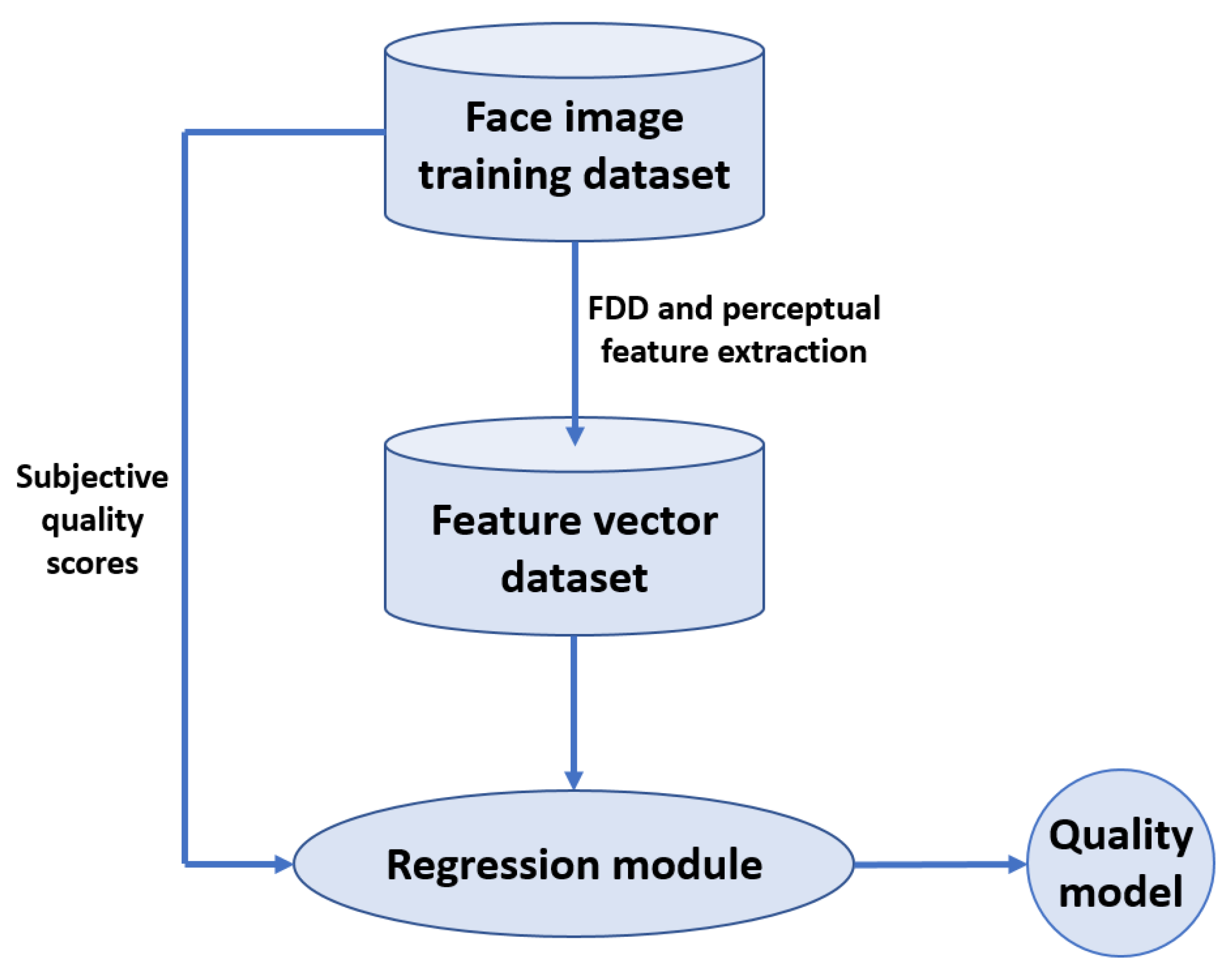
A high-level overview of the proposed FIQA methodology is depicted in Figure 2. There are normally two steps in each machine learning-based IQA system: the training process and the testing phase. Features are taken from a huge set of quality annotated photos during the training phase. This is a typical time-consuming step that is determined by the amount of training pictures used in the training system. The result of the training phase is a quality model obtained with the help of a regression algorithm. Later in the testing phase, this quality model is utilized to evaluate the perceptual quality of previously unseen test images.
Features
In this subsection, the proposed quality-aware Benford’s law-inspired and perceptual features are introduced. The applied features and their descriptions are summarized in Table 1 and discussed in detail in the following paragraphs. As one can observe based on the information provided in Table 1, FDDs are extracted from the wavelet domain, discrete cosine transform coefficients, singular values, and shearlet domain. Further, FDDs are boosted with several popular perceptual features, i.e., colorfulness, the global contrast factor, the dark channel feature, entropy, and the mean of the phase congruency image, which are consistent with human quality judgment [30,31].
Two-dimensional wavelets and filter banks are commonly applied in image processing [38]. Namely, wavelets are a general way to represent and analyze multiresolution images. In the case of one-dimensional discrete wavelet transform (DWT), a one-dimensional input signal is recursively decomposed into approximation and detail at the next lower resolution. The computation of 1D DWT [39] can be described as
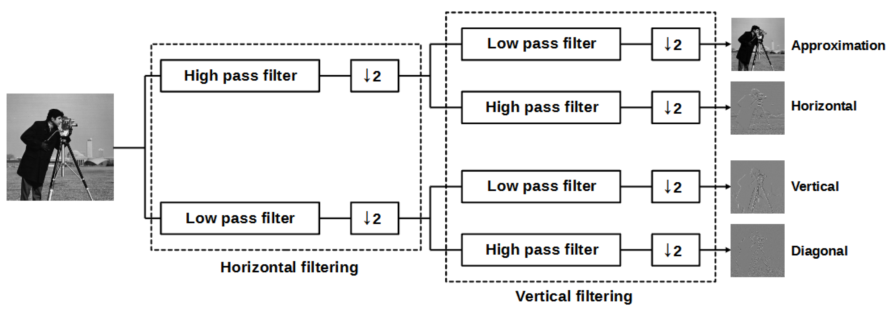
where and are the approximation and detail at level i, respectively. In contrast to 1D DWT, the 2D DWT applies 2D filters, which can be separable or non-separable. Specifically, in the case of separable filters the 2D DWT decomposes an image into an approximation and three detailed images (horizontal, vertical, and diagonal features), as depicted in Figure 3. In this study, Daubechies mother wavelets were applied. Finally, FDDs in horizontal, vertical, and diagonal coefficients were utilized as quality-aware features.
The two-dimensional discrete cosine transform (DCT) is a commonly used tool to compress images [40]. Namely, the two-dimensional DCT can interpreted as a representation for an image in terms of a weighted sum of basis images, since 2D DCT expresses an image I as
where
and represent the 2D DCT coefficients. The FDDs of 2D DCT coefficients were used as quality-aware features.
The singular value decomposition (SVD) is a factorization method that decomposes a matrix into three matrices. Formally, it can be written for every real-valued matrix [41]:
where and are unitary matrices with orthonormal columns and is a diagonal matrix.
The shearlets proposed in 2006 [42] are a mathematical framework and a type of multiscale analysis tool used in signal and image processing. They were introduced as an extension of wavelets to overcome some of their limitations in capturing and representing complex geometrical structures, such as edges, corners, and textures, at different scales and orientations. Shearlets employ a system of shear operations, which involve affine transformations that stretch and rotate a basic analyzing function, called a mother shearlet, to capture the local geometric features of a signal or an image. These shear operations allow shearlets to adapt to the local geometry of the data, enabling them to efficiently represent highly anisotropic features. To define a continuous shearlet system, you need a parabolic scale matrix
and a shear matrix
A continuous shearlet system can be given for as
and the following mapping is the corresponding continuous shearlet transform
In the literature, various ways can be found for discretezing a shearlet system [43]. In this study, one of the most common ones was utilized and can be given as
Subsequently, the discrete shearlet system generated by can be given as
and the following mapping is the corresponding discrete shearlet transform
The FDD of the absolute shearlet coefficients was used as a quality-aware feature.
Colorfulness (CF) refers to the perceived intensity or vibrancy of colors in an image [44]. In other words, it measures how rich and diverse the colors appear in a digital image. A colorful image generally has a wide range of distinct, vivid, and saturated colors. In general, humans tend to perceive more colorful images as visually attractive and engaging [45,46]. For measuring the colorfulness of an image, the model of Hasler and Suesstrunk was adopted in this paper, which can be expressed as
where and denote the mean and standard deviation of matrices in the subscripts. Further, and where R, G, and B denote the red, green, and blue color channels, respectively.
The contrast of an image refers to the difference in brightness, color, or intensity between different elements or regions within the image. It measures the degree of variation and separation between light and dark areas or between colors in the image. In other words, contrast quantifies the distinguishing ability and visual separation of different image features [47]. In this paper, Matkovic et al.’s [48] model—called the global contrast factor (GCF)—was used to quantify the contrast of face images. Formally, it can be expressed as
where
and
Further,
where L denotes the pixel values after a gamma correction .
The dark channel of an image is a concept introduced in the context of haze and fog removal techniques [49]. It represents a low-intensity channel that contains information about the presence of haze or fog in the image. The dark channel is used to estimate the atmospheric light and assist in the restoration of a haze-free image. Specifically, He et al. [50] defined dark pixels as those locations in the image where the value of at least one color channel is low. Consequently, the definition of dark channel can be given formally as
where stands for the value of the color channel . Further, in Equation (20) represents an image patch around pixel x. Based on the above information and denoting the area of the image by S, the definition of the dark channel feature can be given as
The entropy of an image [51] is a measure of the randomness or uncertainty in the distribution of pixel intensities. It quantifies the amount of information or complexity present in the image. Images with a higher entropy have more complex and varied pixel patterns, while images with a lower entropy have more repetitive and predictable pixel patterns. Entropy is typically calculated based on the histogram of pixel intensities in the image:
where represents the probability of intensity n, and the summation is performed over all intensity levels in the histogram.
Phase congruency (PC) analysis [52,53] is commonly used in image processing tasks, such as image feature detection, texture analysis, object recognition, and image quality assessment. Namely, PC is a measure that captures the presence and strength of local structures, such as edges or textures, in an image. It is based on the analysis of phase information in the frequency domain of an image. Originally, PC [54] was defined as
where stands for signal x’s energy and is the nth Fourier amplitude of signal x. Several modifications were carried out in the above equation by Kovesi [55] to introduce noise compensation. Formally, it can be written as
where is the floor function, T is a constant that represents an estimation for the noise level, is a constant used for avoiding division by 0, and are weights for frequency spread. Further, the phase difference can be expressed as
where denotes the nth Fourier component at x and stands for the average phase at x. In this study, the mean of the PC image was used as a perceptual feature.
4. Results
4.1. Evaluation Protocol
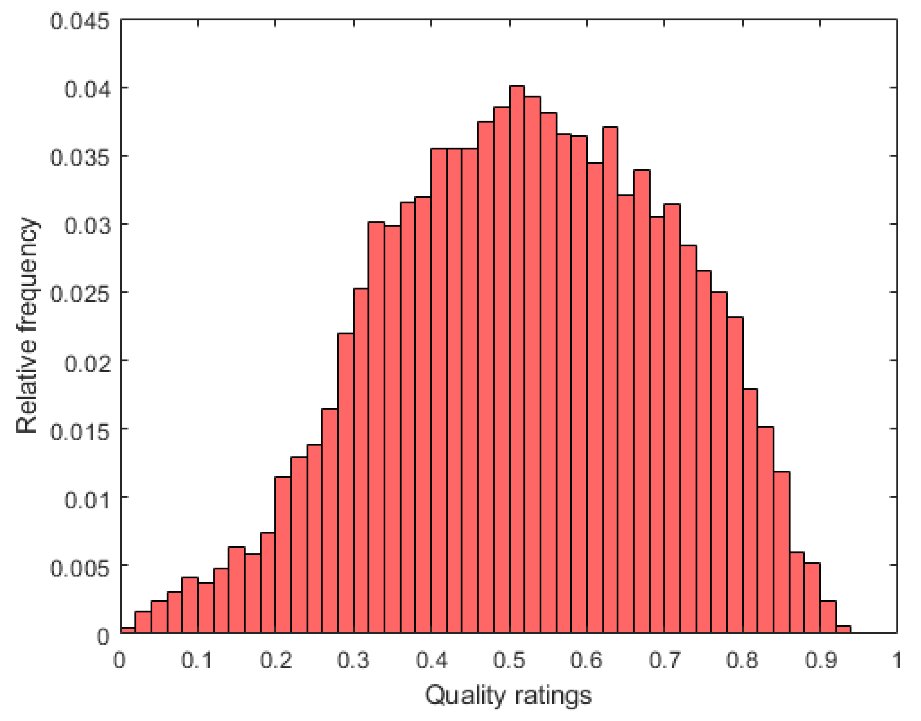
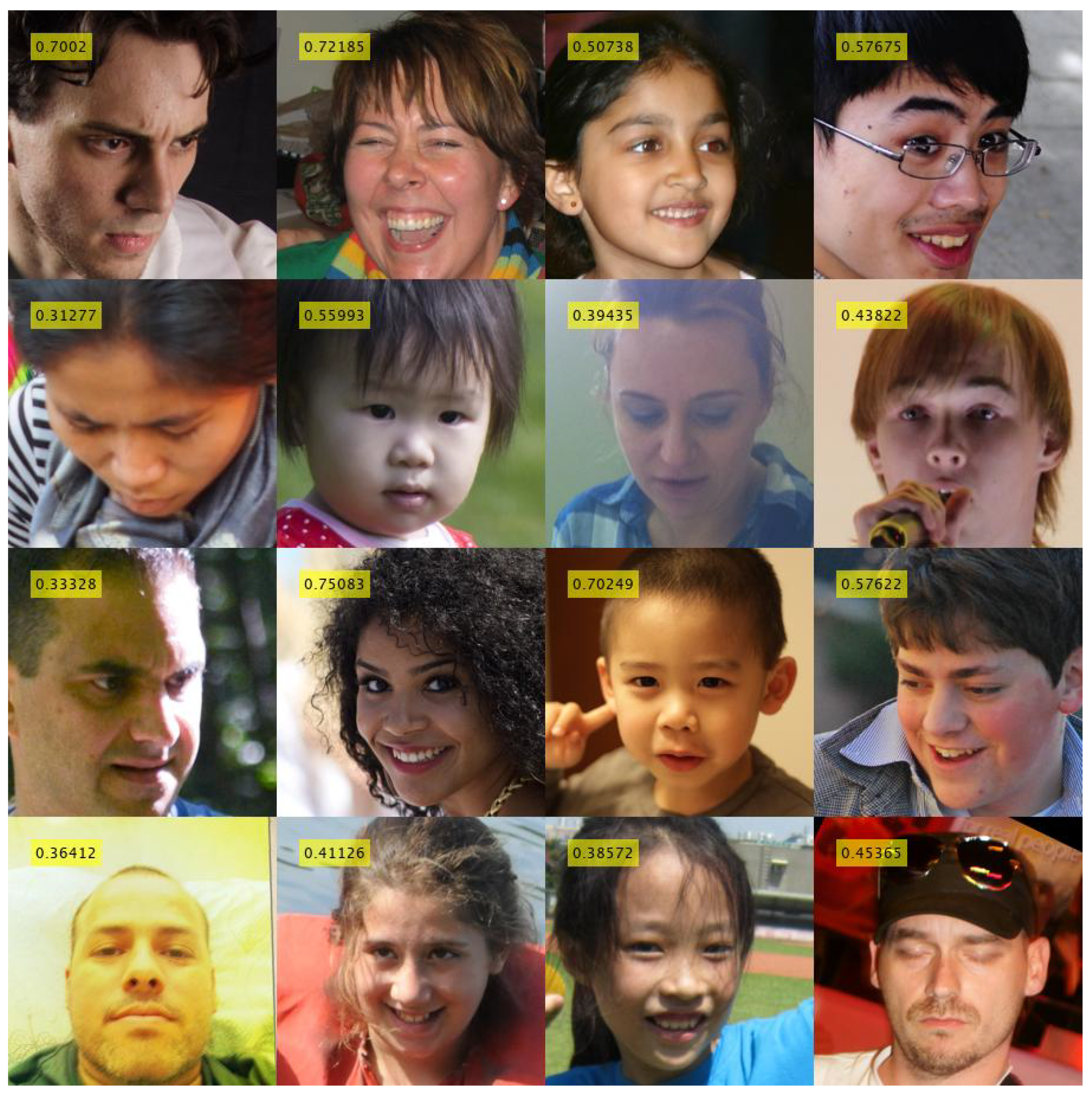
To evaluate the performance of Benford’s law-inspired and perceptual features for FIQA, the generic face image quality assessment 20k database (GFIQA-20k) [56] was utilized, which is currently the largest publicly available one in the literature. The images of this database were sampled from the Yahoo Flickr creative commons 100 million dataset (YFCC100M) [57] and were evaluated by freelancers using the standard five-point absolute category rating [58] scale (bad, poor, fair, good, excellent). On the whole, this database contains 20,000 quality-annotated face images with a resolution. Further, the quality ratings are in the range where a higher rating indicates better visual quality. The distribution of quality ratings is shown in Figure 4. Further, Figure 5 depicts several face images from the GFIQA-20k [56] database with the corresponding quality values.
Machine learning-based methods were evaluated on the GFIQA-20k [56] database as follows. First, the database is randomly divided into training (appx. 80% of images) and test (appx. 20% of images) sets. Second, a machine learning-based FIQA algorithm is trained on the training set. Third, the Pearson’s linear correlation coefficient (PLCC), Spearman’s rank order correlation coefficient (SROCC), and Kendall’s rank order correlation coefficient (KROCC) are computed between the quality labels of the test set and the predicted quality labels. This process is repeated 100 times. Finally, the median PLCC, SROCC, and KROCC values are reported.
4.2. Parameter Study
The goal of the parameter study presented in this subsection is twofold. First, a bunch of regression algorithms are tested to find the one that fits the best to the fusion of Benford’s law-inspired and perceptual features. Second, my goal is to prove with the experiments that all parts of the proposed fusion of Benford’s law-inspired and perceptual features are relevant and important.
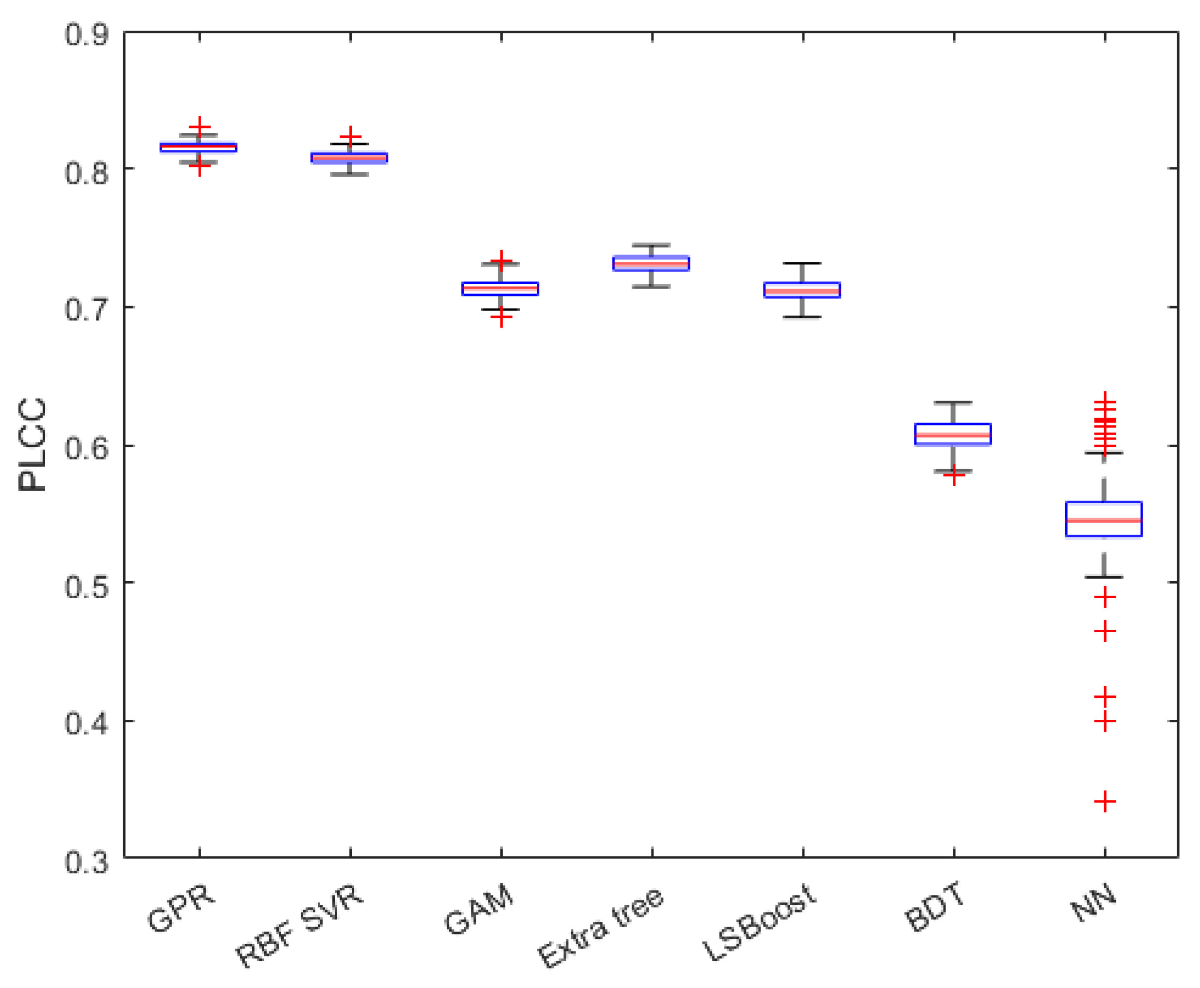
Seven different regression methods, the Gaussian process regressor (GPR) with a rational quadratic kernel function [59], support vector regressor (SVR) with a radial basis function (RBF) [60], generalized additive model (GAM) [61], extra tree [62], LSBoost [63], binary decision tree [64], and regression neural network (NN) [65] with one hidden layer consisting of 10 neurons, were tested to identify the best performing from them. The numerical results with respect to the different regression methods are summarized in Table 2 from which it can be observed that the GPR with a quadratic kernel function performs slightly better than the RBF SVR and significantly better than all the other considered regression algorithms. The obtained PLCC, SROCC, and KROCC values are visually depicted in Figure 6, Figure 7 and Figure 8 in the form of box plots. In each box plot, the median value is denoted by the central mark. Moreover, the 25th and 75th percentiles correspond to the bottom and top edges, respectively. The outliers are represented by red plus signs, and the whiskers extend to the most extreme values, which are not considered outliers.
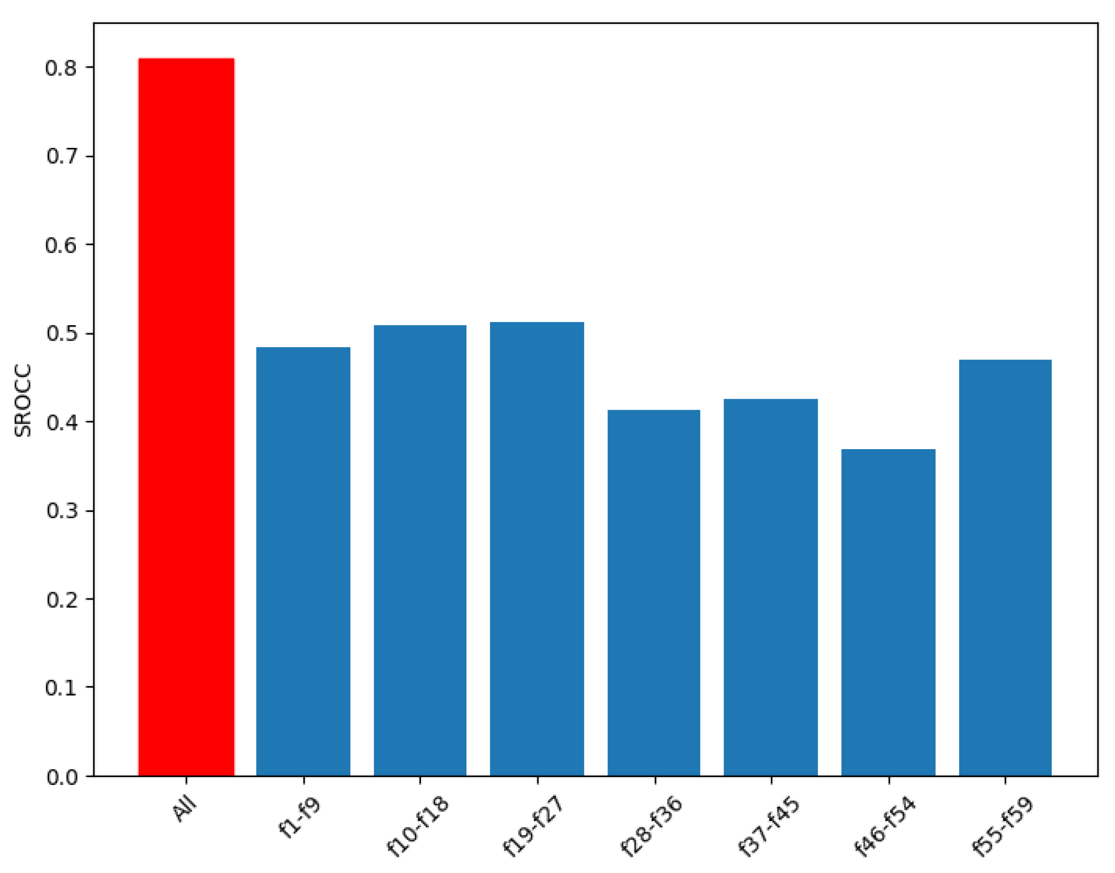
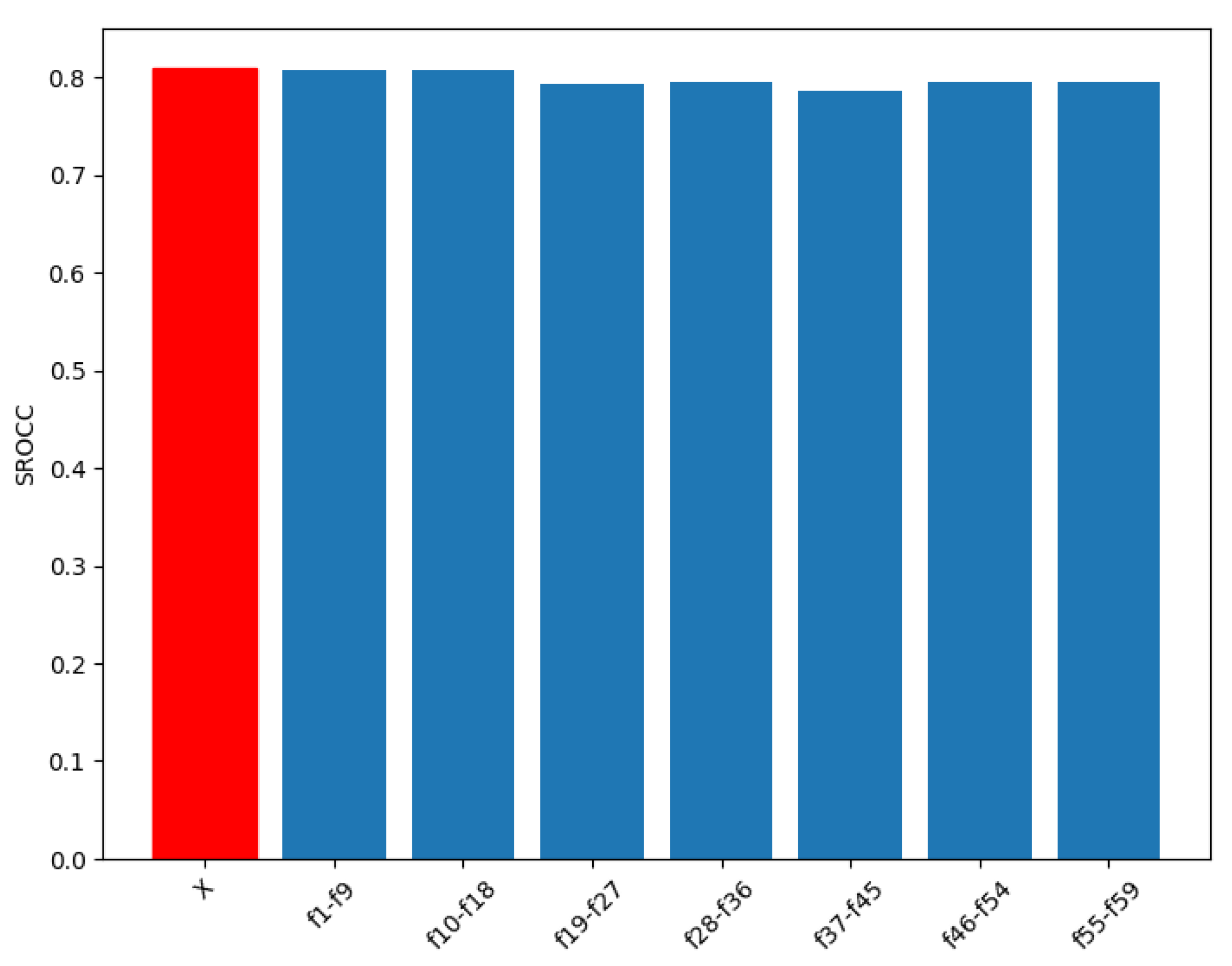
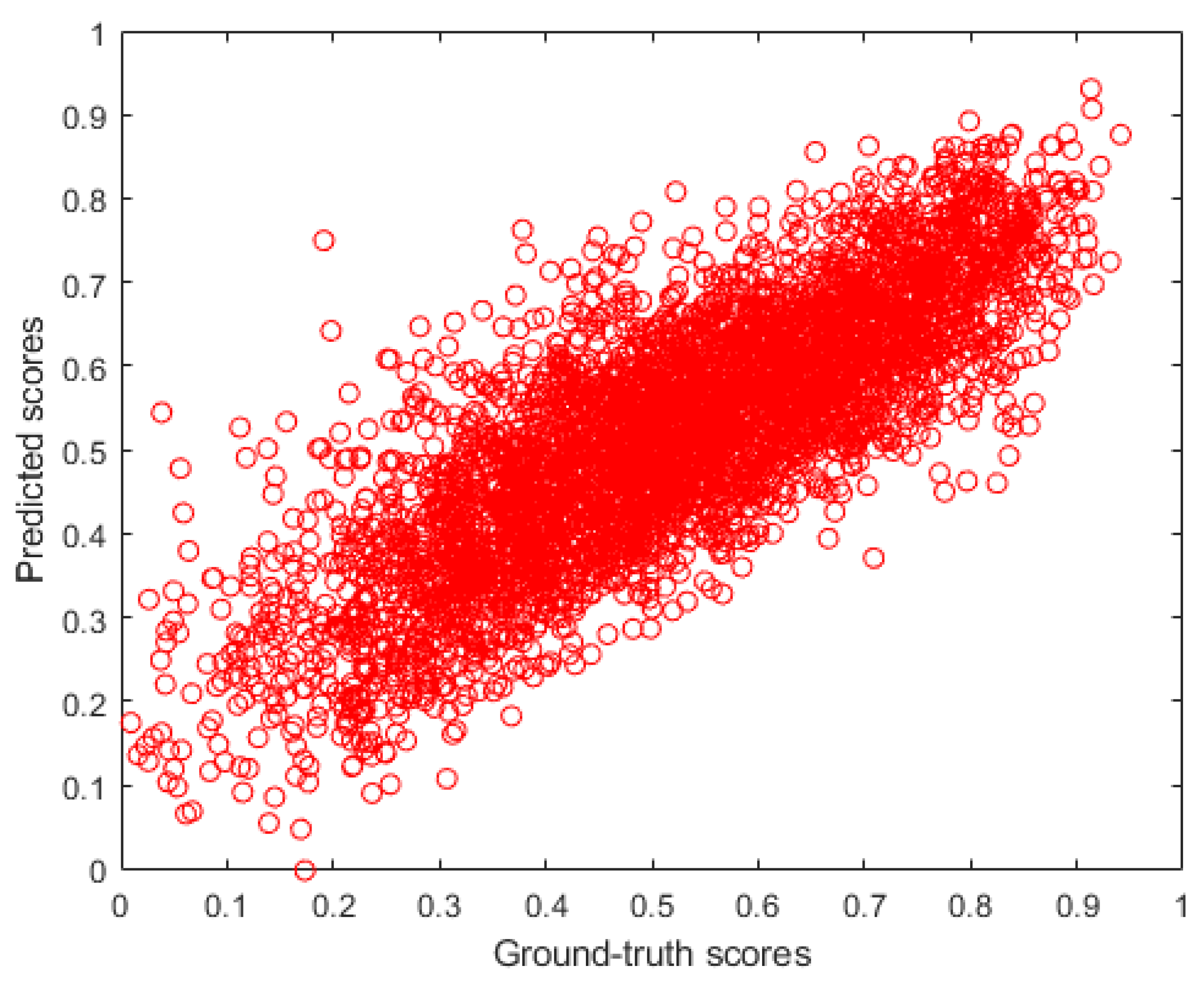
To prove that in the fusion of Benford’s law-inspired and perceptual features for FIQA all parts are important and relevant, the following experiments were applied. First, the performance of the individual parts was measured over 100 random train–test splits. Second, a part of the feature vector was removed, and then the performance of the remaining part was measured over 100 random train–test splits. The results of these two experiment are summarized in Figure 9 and Figure 10 in terms of the median SROCC. From these figures, it can be concluded that the applied Benford’s law-inspired and perceptual features are rather mediocre predictors of face image quality, but their fusion is able to provide a high correlation with the ground-truth quality scores. However, if any part of the proposed feature vector is removed, the correlation strength between the ground-truth and predicted quality scores decreases. Interestingly, some parts of the feature vector (for example, the FDD of singular values), whose removals from the whole feature vector cause a larger performance drop, do not have outstanding individual performances. This indicates that all parts of the feature vector are important and relevant. Moreover, the parts complement each other. Figure 11 depicts a ground-truth versus predicted quality scores scatterplot on a GFIQA-20k [56] test set.
4.3. Comparison to the State-of-the-Art Methods
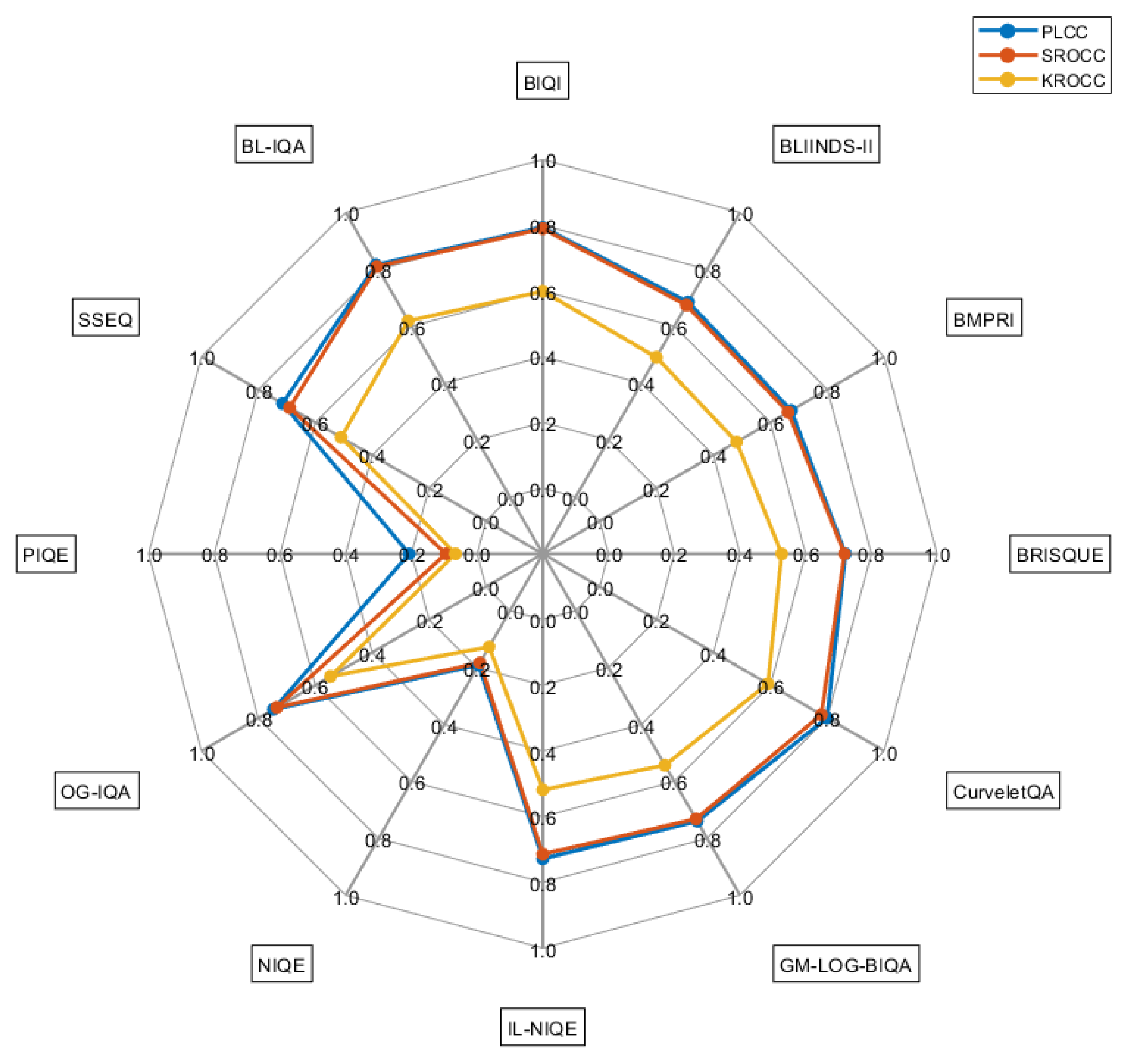
In this subsection, the proposed method relying on Benford’s law-inspired and perceptual features is compared to several other state-of-the-art NR-IQA methods (BIQI [66], BLIINDS-II [67], BMPRI [68], BRISQUE [69], CurveletQA [70], GM-LOG-BIQA [71], IL-NIQE [72], NIQE [73], OG-IQA [74], PIQE [75], SSEQ [76]) on face images. As already mentioned, the results were obtained using the GFIQA-20k [56] benchmark database. Further, all methods using some kind of machine learning method were evaluated using exactly the same protocol. Namely, the database was randomly divided into training (appx. 80% of images) and test sets (appx. 20% of images). Next, the PLCC, SROCC, and KROCC were computed between the labels of tests and the predicted quality scores. This process was repeated 100 times, and the median PLCC, SROCC, and KROCC values are reported in this study. In contrast, opinion-unaware methods, i.e., IL-NIQE [72], NIQE [73], and PIQE [75], were directly evaluated on the entire database without any prior partition of the database, since these methods do not rely on any machine learning techniques. The numerical results of this comparison are summarized in Table 3. From this table, it can be concluded that the fusion of Benford’s law-inspired and perceptual features has proved to be an effective image representation for the estimation of perceptual image quality. Specifically, the proposed BL-IQA is the one from the examined methods that provides the highest median PLCC, SROCC, and KROCC values. Namely, these values are appx. 0.02 higher than those provided by the second-best-performing CurveletQA [70] in terms of the SROCC and KROCC and the BIQI [66] in terms of the PLCC. The numerical results of the comparison to the state-of-the-art methods are visually summarized using radar graphs in Figure 12.
5. Conclusions
In this study, I investigated the effectiveness of Benford’s law-inspired FDD and perceptual features for FIQA. To be more specific, FDDs of multiple image domains, such as wavelet, DCT, singular value, and shearlet domains, were analyzed for FIQA. Our analysis revealed that the FDD of an image domain is a rather mediocre predictor for face image quality. However, the fusion of different FDDs is able to provide a high correlation with the ground-truth quality scores. Moreover, the performance of FDD fusion can be further increased by considering several simple perceptual features, such as colorfulness, the global contrast factor, the dark channel feature, entropy, and phase congruency. Detailed experimental results were presented on the recently published GFIQA-20k [56], which is currently the biggest database containing quality-labeled face images. My future work involves the real-time implementation of FDD feature extraction using CUDA C++ for real-world applications.
Funding
This research received no external funding.
Institutional Review Board Statement
Not applicable.
Informed Consent Statement
Not applicable.
Data Availability Statement
The GFIQA-20k dataset is publically available from http://database.mmsp-kn.de/gfiqa-20k-database.html (accessed on 12 January 2023).
Acknowledgments
I thank the anonymous reviewers and the academic editor for their careful reading of my manuscript and their many insightful comments and suggestions.
Conflicts of Interest
The author declares no conflict of interest.
Abbreviations
The following abbreviations are used in this manuscript:
| BDT | binary decision tree |
| CF | colorfulness |
| DCF | dark channel feature |
| DWT | discrete wavelet transform |
| E | entropy |
| FDD | first digit distribution |
| FIQA | face image quality assessment |
| GAM | generalized additive model |
| GFIQA-20k | generic face image quality assessment 20k database |
| GPR | Gaussian process regression |
| JPEG | joint photographic experts group |
| IQA | image quality assessment |
| KROCC | Kendall’s rank order correlation coefficient |
| NN | neural network |
| PC | phase congruency |
| PLCC | Pearson’s linear correlation coefficient |
| RBF | radial basis function |
| SROCC | Spearman’s rank order correlation coefficient |
| SVD | singular value decomposition |
| SVR | support vector regressor |
| YHCC100M | Yahoo Flickr creative commons 100 million dataset |
References
- Khodabakhsh, A.; Pedersen, M.; Busch, C. Subjective versus objective face image quality evaluation for face recognition. In Proceedings of the 2019 3rd International Conference on Biometric Engineering and Applications, Stockholm, Sweden, 29–31 May 2019; pp. 36–42. [Google Scholar]
- Krizhevsky, A.; Sutskever, I.; Hinton, G.E. Imagenet classification with deep convolutional neural networks. Adv. Neural Inf. Process. Syst. 2012, 25, 1097–1105. [Google Scholar] [CrossRef]
- Boutros, F.; Fang, M.; Klemt, M.; Fu, B.; Damer, N. CR-FIQA: Face image quality assessment by learning sample relative classifiability. In Proceedings of the IEEE/CVF Conference on Computer Vision and Pattern Recognition, Vancouver, BC, Canada, 17–24 June 2023; pp. 5836–5845. [Google Scholar]
- Sang, J.; Lei, Z.; Li, S.Z. Face image quality evaluation for ISO/IEC standards 19794-5 and 29794-5. In Proceedings of the Advances in Biometrics: Third International Conference, ICB 2009, Alghero, Italy, 2–5 June 2009; Proceedings 3. Springer: Berlin/Heidelberg, Germany, 2009; pp. 229–238. [Google Scholar]
- Vignesh, S.; Priya, K.M.; Channappayya, S.S. Face image quality assessment for face selection in surveillance video using convolutional neural networks. In Proceedings of the 2015 IEEE Global Conference on Signal and Information Processing (GlobalSIP), Orlando, FL, USA, 14–16 December 2015; pp. 577–581. [Google Scholar]
- Sellahewa, H.; Jassim, S.A. Image-quality-based adaptive face recognition. IEEE Trans. Instrum. Meas. 2010, 59, 805–813. [Google Scholar] [CrossRef]
- Wasnik, P.; Raja, K.B.; Ramachandra, R.; Busch, C. Assessing face image quality for smartphone based face recognition system. In Proceedings of the 2017 5th International Workshop on Biometrics and Forensics (IWBF), Coventry, UK, 4–5 April 2017; pp. 1–6. [Google Scholar]
- Kuru, K.; Ansell, D. TCitySmartF: A comprehensive systematic framework for transforming cities into smart cities. IEEE Access 2020, 8, 18615–18644. [Google Scholar] [CrossRef]
- Thakur, N.; Han, C.Y. An intelligent ubiquitous activity aware framework for smart home. In Human Interaction, Emerging Technologies and Future Applications III, Proceedings of the 3rd International Conference on Human Interaction and Emerging Technologies: Future Applications (IHIET 2020), Paris, France, 27–29 August 2020; Springer: Berlin/Heidelberg, Germany, 2021; pp. 296–302. [Google Scholar]
- Mir, T.A. The Benford law behavior of the religious activity data. Phys. Stat. Mech. Appl. 2014, 408, 1–9. [Google Scholar] [CrossRef]
- Nigrini, M.J.; Miller, S.J. Benford’s law applied to hydrology data—Results and relevance to other geophysical data. Math. Geol. 2007, 39, 469–490. [Google Scholar] [CrossRef]
- Burke, J.; Kincanon, E. Benford’s law and physical constants: The distribution of initial digits. Am. J. Phys. 1991, 59, 952. [Google Scholar] [CrossRef]
- Alali, F.A.; Romero, S. Benford’s Law: Analyzing a decade of financial data. J. Emerg. Technol. Account. 2013, 10, 1–39. [Google Scholar] [CrossRef]
- Fu, D.; Shi, Y.Q.; Su, W. A generalized Benford’s law for JPEG coefficients and its applications in image forensics. In Proceedings of the Security, Steganography, and Watermarking of Multimedia Contents IX. SPIE, San Jose, CA, USA, 28 January 2007; Volume 6505, pp. 574–584. [Google Scholar]
- Kossovsky, A.E. Benford’s Law: Theory, the General Law of Relative Quantities, and Forensic Fraud Detection Applications; World Scientific: Singapore, 2014; Volume 3. [Google Scholar]
- Mebane, W.R., Jr. Election forensics: Vote counts and Benford’s law. In Proceedings of the Summer Meeting of the Political Methodology Society, UC-Davis, Davis, CA, USA, 20–22 July 2006; Volume 17. [Google Scholar]
- Gonzalez-Garcia, M.J.; Pastor, M.G.C. Benford’s Law and Macroeconomic Data Quality; International Monetary Fund: Washington, DC, USA, 2009. [Google Scholar]
- Li, F.; Han, S.; Zhang, H.; Ding, J.; Zhang, J.; Wu, J. Application of Benford’s law in Data Analysis. J. Phys. Conf. Ser. 2019, 1168, 032133. [Google Scholar] [CrossRef]
- Gottwald, G.A.; Nicol, M. On the nature of Benford’s Law. Phys. Stat. Mech. Appl. 2002, 303, 387–396. [Google Scholar] [CrossRef]
- Sambridge, M.; Tkalčić, H.; Jackson, A. Benford’s law in the natural sciences. Geophys. Res. Lett. 2010, 37, 1–5. [Google Scholar] [CrossRef]
- Zhao, X.; Ho, A.T.; Shi, Y.Q. Image forensics using generalised Benford’s law for accurate detection of unknown JPEG compression in watermarked images. In Proceedings of the 2009 16th International Conference on Digital Signal Processing, Santorini, Greece, 5–7 July 2009; pp. 1–8. [Google Scholar]
- Milani, S.; Tagliasacchi, M.; Tubaro, S. Discriminating multiple JPEG compressions using first digit features. APSIPA Trans. Signal Inf. Process. 2014, 3, e19. [Google Scholar] [CrossRef]
- Pasquini, C.; Boato, G.; Pérez-González, F. Multiple JPEG compression detection by means of Benford-Fourier coefficients. In Proceedings of the 2014 IEEE International Workshop on Information Forensics and Security (WIFS), Atlanta, GA, USA, 3–5 December 2014; pp. 113–118. [Google Scholar]
- Pasquini, C.; Boato, G.; Pérez-González, F. Statistical detection of JPEG traces in digital images in uncompressed formats. IEEE Trans. Inf. Forensics Secur. 2017, 12, 2890–2905. [Google Scholar] [CrossRef]
- Moin, S.S.; Islam, S. Benford’s law for detecting contrast enhancement. In Proceedings of the 2017 Fourth International Conference on Image Information Processing (ICIIP), Shimla, India, 21–23 December 2017; pp. 1–4. [Google Scholar]
- Makrushin, A.; Kraetzer, C.; Neubert, T.; Dittmann, J. Generalized Benford’s law for blind detection of morphed face images. In Proceedings of the 6th ACM Workshop on Information Hiding and Multimedia Security, Innsbruck, Austria, 20–22 June 2018; pp. 49–54. [Google Scholar]
- Wiedemann, O.; Hosu, V.; Lin, H.; Saupe, D. Disregarding the big picture: Towards local image quality assessment. In Proceedings of the 2018 Tenth International Conference on Quality of Multimedia Experience (QoMEX), Cagliari, Italy, 29 May–1 June 2018; pp. 1–6. [Google Scholar]
- Götz-Hahn, F.; Hosu, V.; Lin, H.; Saupe, D. KonVid-150k: A Dataset for No-Reference Video Quality Assessment of Videos in-the-Wild. IEEE Access 2021, 9, 72139–72160. [Google Scholar] [CrossRef]
- Akkaya, E.; Özbek, N. Comparison of the State-of-the-Art Image and Video Quality Assessment Metrics. In Proceedings of the 2021 29th Signal Processing and Communications Applications Conference (SIU), Istanbul, Turkey, 9–11 June 2021; pp. 1–4. [Google Scholar]
- Men, H. Boosting for Visual Quality Assessment with Applications for Frame Interpolation Methods. Ph.D. Thesis, University of Konstanz, Konstanz, Germany, 2022. [Google Scholar]
- Jenadeleh, M. Blind Image and Video Quality Assessment. Ph.D. Thesis, University of Konstanz, Konstanz, Germany, 2018. [Google Scholar]
- Xu, L.; Lin, W.; Kuo, C.C.J. Visual Quality Assessment by Machine Learning; Springer: Berlin/Heidelberg, Germany, 2015. [Google Scholar]
- Schlett, T.; Rathgeb, C.; Henniger, O.; Galbally, J.; Fierrez, J.; Busch, C. Face image quality assessment: A literature survey. ACM Comput. Surv. 2022, 54, 1–49. [Google Scholar] [CrossRef]
- Gao, X.; Li, S.Z.; Liu, R.; Zhang, P. Standardization of face image sample quality. In Proceedings of the Advances in Biometrics: International Conference, ICB 2007, Seoul, Republic of Korea, 27–29 August 2007; Proceedings. Springer: Berlin/Heidelberg, Germany, 2007; pp. 242–251. [Google Scholar]
- Terhorst, P.; Kolf, J.N.; Damer, N.; Kirchbuchner, F.; Kuijper, A. SER-FIQ: Unsupervised estimation of face image quality based on stochastic embedding robustness. In Proceedings of the IEEE/CVF Conference on Computer Vision and Pattern Recognition, Seattle, WA, USA, 13–19 June 2020; pp. 5651–5660. [Google Scholar]
- Ou, F.Z.; Chen, X.; Zhang, R.; Huang, Y.; Li, S.; Li, J.; Li, Y.; Cao, L.; Wang, Y.G. SDD-FIQA: Unsupervised face image quality assessment with similarity distribution distance. In Proceedings of the IEEE/CVF Conference on Computer Vision and Pattern Recognition, Nashville, TN, USA, 20–25 June 2021; pp. 7670–7679. [Google Scholar]
- Babnik, Ž.; Peer, P.; Štruc, V. DifFIQA: Face Image Quality Assessment Using Denoising Diffusion Probabilistic Models. arXiv 2023, arXiv:2305.05768. [Google Scholar]
- Prasad, L.; Iyengar, S.S. Wavelet Analysis with Applications to Image Processing; CRC Press: Boca Raton, FL, USA, 1997. [Google Scholar]
- Mallat, S.G. Multifrequency channel decompositions of images and wavelet models. IEEE Trans. Acoust. Speech Signal Process. 1989, 37, 2091–2110. [Google Scholar] [CrossRef]
- Cintra, R.J.; Bayer, F.M. A DCT approximation for image compression. IEEE Signal Process. Lett. 2011, 18, 579–582. [Google Scholar] [CrossRef]
- Brunton, S.L.; Kutz, J.N. Data-Driven Science and Engineering: Machine Learning, Dynamical Systems, and Control; Cambridge University Press: Cambridge, UK, 2022. [Google Scholar]
- Guo, K.; Kutyniok, G.; Labate, D. Sparse multidimensional representations using anisotropic dilation and shear operators. Wavelets Splines 2006, 14, 189–201. [Google Scholar]
- Häuser, S.; Steidl, G. Fast finite shearlet transform. arXiv 2012, arXiv:1202.1773. [Google Scholar]
- Yendrikhovskij, S.; Blommaert, F.J.; de Ridder, H. Optimizing color reproduction of natural images. In Proceedings of the Color and Imaging Conference. Society for Imaging Science and Technology, Scottsdale, AZ, USA, 17–20 November 1998; Volume 1998, pp. 140–145. [Google Scholar]
- Engeldrum, P.G. Extending image quality models. In Proceedings of the IS and TS Pics Conference. Society for Imaging Science & Technology, Portland, OR, USA, 7–10 April 2002; pp. 65–69. [Google Scholar]
- Yue, G.; Hou, C.; Zhou, T. Blind quality assessment of tone-mapped images considering colorfulness, naturalness, and structure. IEEE Trans. Ind. Electron. 2018, 66, 3784–3793. [Google Scholar] [CrossRef]
- Peli, E. Contrast in complex images. JOSA A 1990, 7, 2032–2040. [Google Scholar] [CrossRef] [PubMed]
- Matkovic, K.; Neumann, L.; Neumann, A.; Psik, T.; Purgathofer, W. Global contrast factor—A new approach to image contrast. In Proceedings of the Computational Aesthetics 2005: Eurographics Workshop on Computational Aesthetics in Graphics, Visualization and Imaging 2005, Girona, Spain, 18–20 May 2005; pp. 159–167. [Google Scholar]
- Lee, S.; Yun, S.; Nam, J.H.; Won, C.S.; Jung, S.W. A review on dark channel prior based image dehazing algorithms. Eurasip J. Image Video Process. 2016, 2016, 4. [Google Scholar] [CrossRef]
- He, K.; Sun, J.; Tang, X. Single image haze removal using dark channel prior. IEEE Trans. Pattern Anal. Mach. Intell. 2010, 33, 2341–2353. [Google Scholar] [PubMed]
- Gull, S.F.; Skilling, J. Maximum entropy method in image processing. IET 1984, 131, 646–659. [Google Scholar] [CrossRef]
- Kovesi, P. Image features from phase congruency. Videre J. Comput. Vis. Res. 1999, 1, 1–26. [Google Scholar]
- Kovesi, P. Phase congruency: A low-level image invariant. Psychol. Res. 2000, 64, 136–148. [Google Scholar] [CrossRef] [PubMed]
- Morrone, M.C.; Ross, J.; Burr, D.C.; Owens, R. Mach bands are phase dependent. Nature 1986, 324, 250–253. [Google Scholar] [CrossRef]
- Kovesi, P. Phase congruency detects corners and edges. In Proceedings of the Australian Pattern Recognition Society Conference: DICTA, Sydney, Australia, 10–12 December 2003; Volume 2003. [Google Scholar]
- Su, S.; Lin, H.; Hosu, V.; Wiedemann, O.; Sun, J.; Zhu, Y.; Liu, H.; Zhang, Y.; Saupe, D. Going the Extra Mile in Face Image Quality Assessment: A Novel Database and Model. arXiv 2022, arXiv:2207.04904. [Google Scholar] [CrossRef]
- Thomee, B.; Shamma, D.A.; Friedland, G.; Elizalde, B.; Ni, K.; Poland, D.; Borth, D.; Li, L.J. YFCC100M: The new data in multimedia research. Commun. ACM 2016, 59, 64–73. [Google Scholar] [CrossRef]
- Saupe, D.; Hahn, F.; Hosu, V.; Zingman, I.; Rana, M.; Li, S. Crowd workers proven useful: A comparative study of subjective video quality assessment. In Proceedings of the QoMEX 2016: 8th International Conference on Quality of Multimedia Experience, Lisbon, Portugal, 6–8 June 2016. [Google Scholar]
- Seeger, M. Gaussian processes for machine learning. Int. J. Neural Syst. 2004, 14, 69–106. [Google Scholar] [CrossRef]
- Smola, A.J.; Schölkopf, B. A tutorial on support vector regression. Stat. Comput. 2004, 14, 199–222. [Google Scholar] [CrossRef]
- Lou, Y.; Caruana, R.; Gehrke, J. Intelligible models for classification and regression. In Proceedings of the 18th ACM SIGKDD International Conference on Knowledge Discovery and Data Mining, Beijing, China, 12–16 August 2012; pp. 150–158. [Google Scholar]
- Geurts, P.; Ernst, D.; Wehenkel, L. Extremely randomized trees. Mach. Learn. 2006, 63, 3–42. [Google Scholar] [CrossRef]
- Breiman, L. Random forests. Mach. Learn. 2001, 45, 5–32. [Google Scholar] [CrossRef]
- Loh, W.Y. Regression tress with unbiased variable selection and interaction detection. Stat. Sin. 2002, 12, 361–386. [Google Scholar]
- Wright, S.; Nocedal, J. Numerical Optimization; Springer Science: Berlin/Heidelberg, Germany, 1999; Volume 35, p. 7. [Google Scholar]
- Moorthy, A.; Bovik, A. A modular framework for constructing blind universal quality indices. IEEE Signal Process. Lett. 2009, 17, 7. [Google Scholar]
- Saad, M.A.; Bovik, A.C. Blind quality assessment of videos using a model of natural scene statistics and motion coherency. In Proceedings of the 2012 Conference Record of the Forty Sixth Asilomar Conference on Signals, Systems and Computers (ASILOMAR), Pacific Grove, CA, USA, 4–7 November 2012; pp. 332–336. [Google Scholar]
- Min, X.; Zhai, G.; Gu, K.; Liu, Y.; Yang, X. Blind image quality estimation via distortion aggravation. IEEE Trans. Broadcast. 2018, 64, 508–517. [Google Scholar] [CrossRef]
- Mittal, A.; Moorthy, A.K.; Bovik, A.C. No-reference image quality assessment in the spatial domain. IEEE Trans. Image Process. 2012, 21, 4695–4708. [Google Scholar] [CrossRef]
- Liu, L.; Dong, H.; Huang, H.; Bovik, A.C. No-reference image quality assessment in curvelet domain. Signal Process. Image Commun. 2014, 29, 494–505. [Google Scholar] [CrossRef]
- Xue, W.; Mou, X.; Zhang, L.; Bovik, A.C.; Feng, X. Blind image quality assessment using joint statistics of gradient magnitude and Laplacian features. IEEE Trans. Image Process. 2014, 23, 4850–4862. [Google Scholar] [CrossRef]
- Zhang, L.; Zhang, L.; Bovik, A.C. A feature-enriched completely blind image quality evaluator. IEEE Trans. Image Process. 2015, 24, 2579–2591. [Google Scholar] [CrossRef]
- Mittal, A.; Soundararajan, R.; Bovik, A.C. Making a “completely blind” image quality analyzer. IEEE Signal Process. Lett. 2012, 20, 209–212. [Google Scholar] [CrossRef]
- Liu, L.; Hua, Y.; Zhao, Q.; Huang, H.; Bovik, A.C. Blind image quality assessment by relative gradient statistics and adaboosting neural network. Signal Process. Image Commun. 2016, 40, 1–15. [Google Scholar] [CrossRef]
- Venkatanath, N.; Praneeth, D.; Bh, M.C.; Channappayya, S.S.; Medasani, S.S. Blind image quality evaluation using perception based features. In Proceedings of the 2015 Twenty First National Conference on Communications (NCC), Maharashtra, India, 27 February–1 March 2015; pp. 1–6. [Google Scholar]
- Liu, L.; Liu, B.; Huang, H.; Bovik, A.C. No-reference image quality assessment based on spatial and spectral entropies. Signal Process. Image Commun. 2014, 29, 856–863. [Google Scholar] [CrossRef]
Figure 1.
Relative frequency of leading digits based on the prediction of Benford’s law.

Figure 2.
Process for investigating the effectiveness of Benford’s law-inspired and perceptual features for face image quality assessment.
Figure 2.
Process for investigating the effectiveness of Benford’s law-inspired and perceptual features for face image quality assessment.

Figure 3.
Illustration of two-dimensional discrete wavelet transform.

Figure 4.
Measured empirical distribution of GFIQA-20k’s [56] quality ratings.
Figure 4.
Measured empirical distribution of GFIQA-20k’s [56] quality ratings.

Figure 5.
Sample images from GFIQA-20k [56]. Quality ratings are printed on the face images in the upper left corners.
Figure 5.
Sample images from GFIQA-20k [56]. Quality ratings are printed on the face images in the upper left corners.

Figure 6.
PLCC values of different regression methods in the form of box plots. Measured over 100 random train–test splits on GFIQA-20k [56]. In each box plot, the median value is denoted by the central mark. Moreover, the 25th and 75th percentiles correspond to the bottom and top edges, respectively. The outliers are represented by red plus signs, and the whiskers extend to the most extreme values, which are not considered outliers.

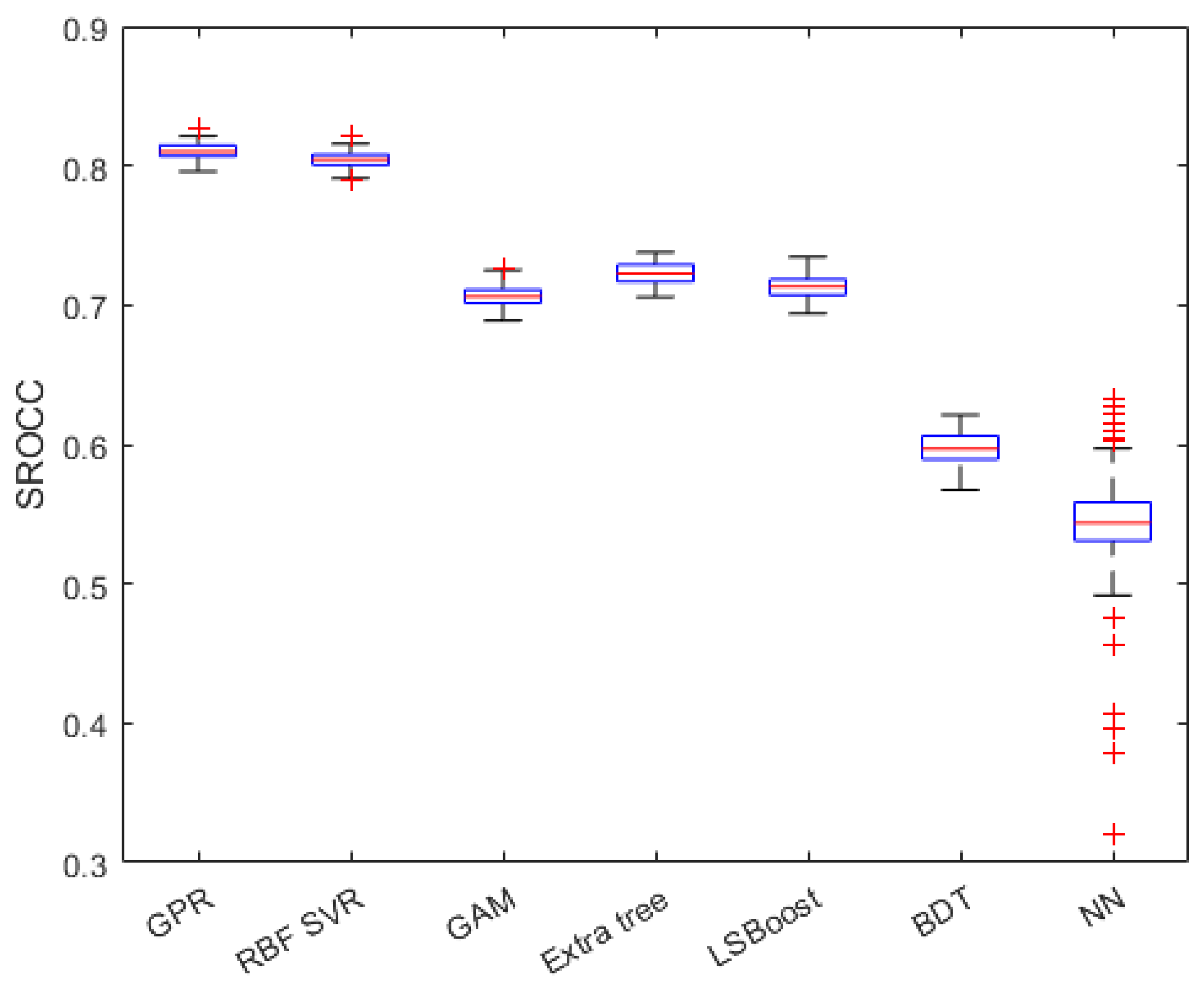
Figure 7.
SROCC values of different regression methods in the form of box plots. Measured over 100 random train–test splits on GFIQA-20k [56]. In each box plot, the median value is denoted by the central mark. Moreover, the 25th and 75th percentiles correspond to the bottom and top edges, respectively. The outliers are represented by red plus signs, and the whiskers extend to the most extreme values, which are not considered as outliers.

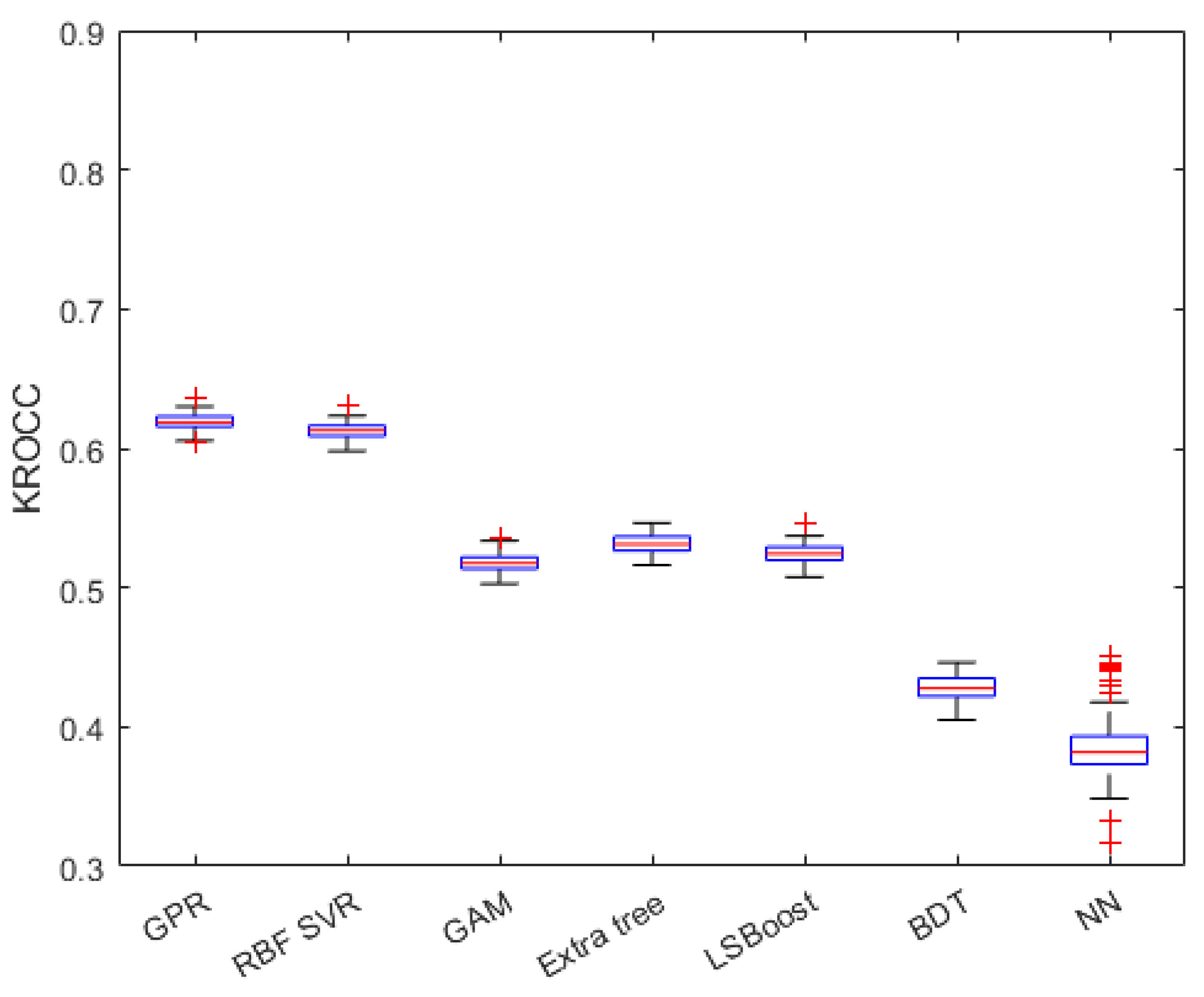
Figure 8.
KROCC values of different regression methods in the form of box plots. Measured over 100 random train–test splits on GFIQA-20k [56]. In each box plot, the median value is denoted by the central mark. Moreover, the 25th and 75th percentiles correspond to the bottom and top edges, respectively. The outliers are represented by red plus signs, and the whiskers extend to the most extreme values, which are not considered as outliers.

Figure 9.
Performance comparison of FDD and perceptual features. Median SROCC values were measured over 100 random train–test splits on GFIQA-20k [56].
Figure 9.
Performance comparison of FDD and perceptual features. Median SROCC values were measured over 100 random train–test splits on GFIQA-20k [56].

Figure 10.
Performance of the proposed feature vector in cases where a part of the feature vector was removed. The performance of the whole feature vector is denoted by ’X’. Median SROCC values were measured over 100 random train–test splits on GFIQA-20k [56].
Figure 10.
Performance of the proposed feature vector in cases where a part of the feature vector was removed. The performance of the whole feature vector is denoted by ’X’. Median SROCC values were measured over 100 random train–test splits on GFIQA-20k [56].

Figure 11.
Ground-truth vs. predicted quality scores scatterplot on a GFIQA-20k [56] test set.
Figure 11.
Ground-truth vs. predicted quality scores scatterplot on a GFIQA-20k [56] test set.

Figure 12.
Radar graph for the visual comparison of median PLCC, SROCC, and KROCC values obtained on GFIQA-20k [56] after 100 random train–test splits.
Figure 12.
Radar graph for the visual comparison of median PLCC, SROCC, and KROCC values obtained on GFIQA-20k [56] after 100 random train–test splits.


Table 1.
Quality-aware features applied in the proposed FIQA method.
| Feature Number | Description | Number of Features |
|---|---|---|
| f1–f9 | FDD of horizontal wavelet coefficients | 9 |
| f10–f18 | FDD of vertical wavelet coefficients | 9 |
| f19–f27 | FDD of diagonal wavelet coefficients | 9 |
| f28–f36 | FDD of DCT coefficients | 9 |
| f37–f45 | FDD of singular values | 9 |
| f46–f54 | FDD of absolute shearlet coefficients | 9 |
| f55–f59 | Perceptual features (colorfulness, global contrast factor, dark channel feature, entropy, mean of phase congruency) | 5 |
Table 2.
Comparison of different regression modules in terms of median PLCC, SROCC, and KROCC, which were measured on GFIQA-20k [56] over 100 random train–test splits. The standard deviation values are given in parentheses.
Table 2.
Comparison of different regression modules in terms of median PLCC, SROCC, and KROCC, which were measured on GFIQA-20k [56] over 100 random train–test splits. The standard deviation values are given in parentheses.
| Regressor | PLCC | SROCC | KROCC |
|---|---|---|---|
| GPR | 0.816 (0.005) | 0.810 (0.006) | 0.619 (0.006) |
| RBF SVR | 0.808 (0.005) | 0.805 (0.006) | 0.613 (0.006) |
| GAM | 0.713 (0.007) | 0.706 (0.008) | 0.518 (0.007) |
| Extra tree | 0.731 (0.007) | 0.723 (0.008) | 0.531 (0.007) |
| LSBoost | 0.711 (0.008) | 0.713 (0.008) | 0.524 (0.007) |
| BDT | 0.607 (0.012) | 0.597 (0.012) | 0.428 (0.009) |
| NN | 0.545 (0.116) | 0.544 (0.069) | 0.382 (0.050) |
Table 3.
Comparison to other state-of-the-art algorithms using GFIQA-20k [56] database. Median PLCC, SROCC, and KROCC values were measured over 100 random train–test splits. The best results are typed in red, the second-best results are typed green, and the third-best results are given in blue.
Table 3.
Comparison to other state-of-the-art algorithms using GFIQA-20k [56] database. Median PLCC, SROCC, and KROCC values were measured over 100 random train–test splits. The best results are typed in red, the second-best results are typed green, and the third-best results are given in blue.
| Method | PLCC | SROCC | KROCC |
|---|---|---|---|
| BIQI [66] | 0.794 | 0.790 | 0.599 |
| BLIINDS-II [67] | 0.685 | 0.674 | 0.491 |
| BMPRI [68] | 0.673 | 0.662 | 0.481 |
| BRISQUE [69] | 0.721 | 0.718 | 0.527 |
| CurveletQA [70] | 0.799 | 0.779 | 0.591 |
| GM-LOG-BIQA [71] | 0.740 | 0.732 | 0.543 |
| IL-NIQE [72] | 0.728 | 0.714 | 0.518 |
| NIQE [73] | 0.191 | 0.183 | 0.127 |
| OG-IQA [74] | 0.747 | 0.735 | 0.546 |
| PIQE [75] | 0.207 | 0.095 | 0.066 |
| SSEQ [76] | 0.715 | 0.690 | 0.509 |
| BL-IQA | 0.816 | 0.810 | 0.619 |
Disclaimer/Publisher’s Note: The statements, opinions and data contained in all publications are solely those of the individual author(s) and contributor(s) and not of MDPI and/or the editor(s). MDPI and/or the editor(s) disclaim responsibility for any injury to people or property resulting from any ideas, methods, instructions or products referred to in the content. |
© 2023 by the author. Licensee MDPI, Basel, Switzerland. This article is an open access article distributed under the terms and conditions of the Creative Commons Attribution (CC BY) license (https://creativecommons.org/licenses/by/4.0/).
Share and Cite
MDPI and ACS Style
Varga, D. Benford’s Law and Perceptual Features for Face Image Quality Assessment. Signals 2023, 4, 859-876. https://doi.org/10.3390/signals4040047
AMA Style
Varga D. Benford’s Law and Perceptual Features for Face Image Quality Assessment. Signals. 2023; 4(4):859-876. https://doi.org/10.3390/signals4040047
Chicago/Turabian StyleVarga, Domonkos. 2023. "Benford’s Law and Perceptual Features for Face Image Quality Assessment" Signals 4, no. 4: 859-876. https://doi.org/10.3390/signals4040047