High-Quality and Reproducible Automatic Drum Transcription from Crowdsourced Data

Abstract

Within the broad problem known as automatic music transcription, we considered the specific task of automatic drum transcription (ADT). This is a complex task that has recently shown significant advances thanks to deep learning (DL) techniques. Most notably, massive amounts of labeled data obtained from crowds of annotators have made it possible to implement large-scale supervised learning architectures for ADT. In this study, we explored the untapped potential of these new datasets by addressing three key points: First, we reviewed recent trends in DL architectures and focused on two techniques, self-attention mechanisms and tatum-synchronous convolutions. Then, to mitigate the noise and bias that are inherent in crowdsourced data, we extended the training data with additional annotations. Finally, to quantify the potential of the data, we compared many training scenarios by combining up to six different datasets, including zero-shot evaluations. Our findings revealed that crowdsourced datasets outperform previously utilized datasets, and regardless of the DL architecture employed, they are sufficient in size and quality to train accurate models. By fully exploiting this data source, our models produced high-quality drum transcriptions, achieving state-of-the-art results. Thanks to this accuracy, our work can be more successfully used by musicians (e.g., to learn new musical pieces by reading, or to convert their performances to MIDI) and researchers in music information retrieval (e.g., to retrieve information from the notes instead of audio, such as the rhythm or structure of a piece).

1. Introduction

In this work, we tackled the problem of generating an automatic music transcription (AMT) of a given audio recording. Depending on the desired content of the transcription and the nature of the audio recording, there exist different formulations of this problem. We focused on the transcription of drum onsets (both their timings and instruments involved), a task known as automatic drum transcription (ADT) in the context of polyphonic audio tracks—tracks that contain both melodic and drum instruments—since they represent the majority of musical tracks in the real world (e.g., any radio song). This specification of ADT is a challenging problem known as drum transcription in the presence of melodic instruments (DTM).

The main challenge of DTM comes from the fact that multiple sounds can be associated with one instrument, and the same sound can be associated with multiple instruments. On the one hand, something that is true for AMT as a whole, any instrument can be played with different techniques (e.g., rimshots, ghost notes, and flams) and undergo distinct recording procedures (depending, for example, on the recording equipment used, the characteristics of the instruments, and the audio effects added during the post-processing sessions). On the other hand, something that is specific to polyphonic recordings seen in DTM, melodic and percussive instruments can overlap and mask each other (e.g., the bass guitar may hide a bass drum onset) or have similar sounds, thus creating confusion between instruments (e.g., a bass drum may be misinterpreted for a low tom or yield to the perception of an extra low tom on top of it).

Due to this complexity, the most promising methods for DTM, as identified by the review work of Wu et al. [1], use supervised deep learning (DL) algorithms—large models trained with labeled datasets. However, despite their good performance, there is still a large margin for improvement. In fact, it is acknowledged that these algorithms are limited by the amount of training data available; by contrast, due to the fact that their generation is labor-intensive, existing datasets are usually small. Furthermore, because data are often copyrighted, datasets are made publicly available only in very few cases. As a result, the available data do not cover the huge diversity that is found in music and is needed to train DL algorithms to reach their full potential.

In response to this data paucity, most of the approaches either tackle a simplified variant of DTM or rely on techniques other than supervised learning. For example, the problem can be simplified by restricting the desired content of the transcription to a vocabulary that includes only the three most common drum instruments, i.e., the bass drum, snare drum, and hi-hat, or by using techniques such as transfer or unsupervised learning that can mitigate the lack of training data—indeed, one of the most competitive methods, proposed by Vogl et al., is based on transfer learning from a large amount of synthetic data [2].

Nevertheless, limiting the scope of the problem and mitigating the data paucity are not satisfying solutions. Instead, it would be preferable to increase the amount of training data, which has been shown to be possible with two recent large-scale datasets: ADTOF [3] and A2MD [4]. Thanks to the large amount of crowdsourced, publicly available, non-synthetic data from the Internet, these datasets have improved the supervised training of DTM models. However, these datasets have not yet been well exploited for three reasons: no exploration of an optimal DL architecture has been conducted; due to crowdsourcing, the data contain discrepancies and are biased to specific music genres; only a few training procedures have been evaluated. Our goal was to explore how these datasets can be efficiently used by addressing all three aforementioned issues:

• To identify an optimal architecture, we compared multiple architectures exploiting recent techniques in DL;
• To mitigate noise and bias in crowdsourced datasets, we curated a new dataset to be used conjointly with existing ones;
• To evaluate the datasets, we compared multiple training procedures by combining different mixtures of data.

We now present our three contributions in detail.

Before the current work, as the experiments involving ADTOF and A2MD were limited to the curation and validation of the datasets, different DL architectures able to leverage this data had still to be evaluated. In fact, only one architecture had been implemented with each dataset, without comparison to others. Here, instead, we present and assess a total of four different architectures that exploit two recent techniques: tatum synchronicity and self-attention mechanisms [5,6,7]. In terms of accuracy (the F-measure), we found that all these architectures are practically equivalent; hence, we concluded that, to a large extent, the favorable performance of our algorithm is not due to these recent improvements in DL.

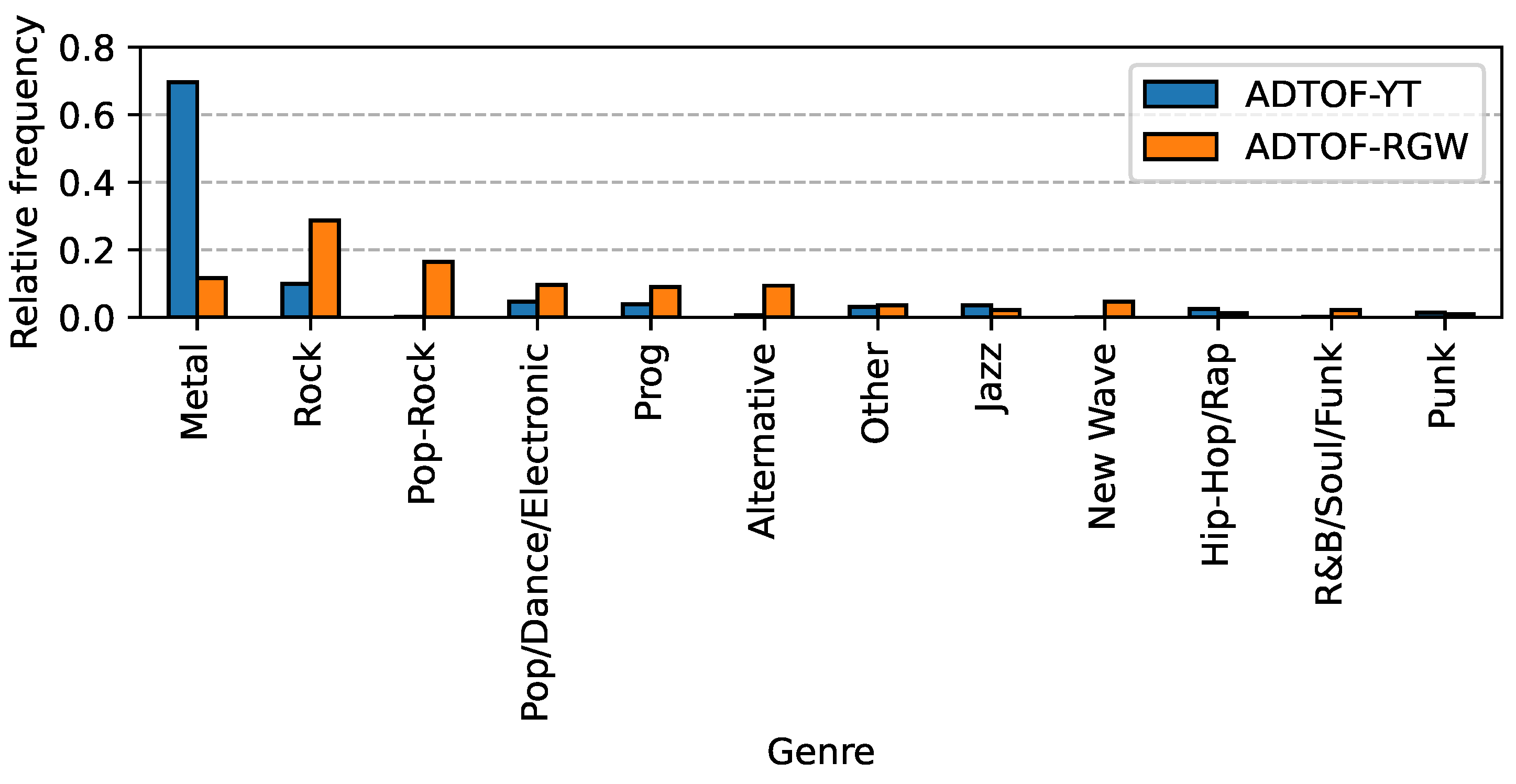
Second, recent studies involving ADTOF and A2MD showed that the crowdsourced nature of these datasets is likely to hinder the performance of the models trained on them. On the one hand, because different annotators have different levels of expertise, there are discrepancies in the annotations. To address this issue, we built a new dataset (adopting the same cleansing process employed in ADTOF), this time using tracks with high-quality annotations selected by the community of annotators. We named this set ADTOF-YT. The first part of the name (“ADTOF”) is a reference to the cleansing process, and the second part (“YT”) comes from the fact that many of the tracks curated are showcased on streaming platforms like YouTube. On the other hand, because this new set and ADTOF are biased toward different musical genres selected by the crowd, a model trained on either of them will suffer from a generalization error. To counter this issue, we trained on both sets at the same time; we then showed that the increased quantity and diversity of training data contributed largely to the performance of our algorithm.

Last, crowdsourced datasets have only been used to train models that were evaluated in a “zero-shot” setting (i.e., the models were evaluated on datasets that were not used for training), whereas the state-of-the-art model used as a reference was not (i.e., the model was evaluated on different divisions of the same datasets used for training). A zero-shot evaluation is more desirable than only splitting the datasets into “training” and “test” partitions because of the homogeneity inherent in the curation process; however, zero-shot evaluation is also a more challenging task. Since the crowdsourced datasets were previously evaluated only in zero-shot studies, their performance in non-zero-shot scenarios is still unknown. As a consequence, in this work we compared the training procedures as follows: We trained on a mixture of commonly used datasets, first with, and then without, a chosen dataset each time. Thus, we revealed both the contribution of the chosen dataset to the performance of the model when it was added to the training data, and the generalization capabilities of the model on the dataset when it was left out.

The remainder of this article is organized as follows: First, we present previous works on ADT in Section 2. We then describe the materials and methods of our experiments on the deep learning architectures and training procedures in Section 3. This part also presents the new dataset we curated. We continue by presenting and discussing the results in Section 4, before concluding and outlining future work in Section 5.

2. Related Works

ADT comprises a large body of research, of which Wu et al. [1] conducted an extensive review up to 2018. In their work, they analyzed three types of ADT with increasing levels of complexity: drum transcription of drum-only recordings (DTD); drum transcription in the presence of percussion (DTP) with additional, non-transcribed, percussion instruments; and drum transcription in the presence of melodic instruments (DTM), with “full-mixture music such as pop, rock, and jazz recordings”. Wu et al. reported that “reliable performances can be expected from the state-of-the-art systems” only for DTD, the simplest of the three. Indeed, as the tasks become more complex, as with DTP and even more so with DTM, there is “room for future improvement”. The authors also noticed that, among all the evaluated algorithms, deep learning (DL) methods seemed “to be the most promising approaches”, as long as sufficient training data are provided. This is something that Jacques and Roebel also realized while comparing multiple methods for DTM [8].

Since 2018, many other attempts at improvement (already identified by Wu et al.) have been pursued. A summary of the works concerned with enhancing ADT is provided in

Table 1. Overview of works related to ADT since 2018.

Year	Work	Task	Voc.	Architecture	Training Proc.	Training Data
2018	Cartwriht and Bello [9]	DTM + BD	14	CRNN	Supervised	ENST, MDB, RBMA, SDDS 1, etc.
2018	Jacques and Roebel [8]	DTM	3	CNN	Supervised	ENST, RWC 1
2018	Vogl et al. [2]	DTM	18	CRNN	Supervised	ENST, MDB, RBMA, TMIDT 1
2019	Choi and Cho [10]	DTP	11	CRNN	Unsupervised	In-house dataset
2019	Jacques and Roebel [11]	DTM	3	CNN	Supervised	MIREX 2018 2
2020	Callender et al. [12]	DTD + V	7	CRNN	Supervised	E-GMD 1,2
2020	Ishizuka et al. [5]	DTM	3	CRNN, LM	Supervised	RWC 3,4
2020	Manilow et al. [13]	MIT + SS	88	RNN	Supervised	MAPS, Slakh 1, GuitarSet
2020	Wang et al. [14]	DTM	Open	CNN	Few-shot	Slakh 1
2021	Cheuk et al. [15]	MIT	88	CNN-SelfAtt	Semi-supervised	MAPS 1, MusicNet
2021	Gardner et al. [16]	MIT	128	SelfAtt	Supervised	Cerberus4 1, Slakh 1, etc.
2021	Ishizuka et al. [6]	DTM	3	CNN-SelfAtt, LM	Supervised	Slakh 1,4, RWC 3,4
2021	Wei et al. [4]	DTM	3	CNN-SelfAtt	Supervised	A2MD (TS)
2021	Zehren et al. [3]	DTM	5	CRNN	Supervised	ADTOF
2022	Simon et al. [17]	MIT	128	SelfAtt	Self-supervised	In-house dataset, Cerberus4 1, etc.
2022	Cheuk et al. [18]	MIT+SS	128	CRNN	Supervised	Slakh 1

¹ Synthetic dataset. ² Data augmentation. ³ Source separation. ⁴ Tatum synchronicity. Acronyms: BD, beat detection; V, velocity estimation;MIT, multi-instrument transcription; SS, source separation; LM, language model.

, and they are described below by focusing first on the tasks and vocabulary included and then, separately, on the architectures, training procedures, and training data employed.

2.1. Tasksand Vocabulary

As the studies on ADT have evolved, we have witnessed an increasing interest in attempting thorough tasks that deliver more detailed transcriptions. These can be obtained through more versatile algorithms than those used in tasks such as DTD with a three-instrument vocabulary. As an illustration, most of the recent works in Table 1 focused on either DTM or multi-instrument transcriptions (MITs, where both percussive and melodic instruments are transcribed). In another example, Callender et al. tried to estimate the velocity (dynamics) of the drum notes [12] in drum-only recordings and showed that velocity played an important role in the perception of the quality of the transcription. Similarly, many works have tried to enlarge the typical three-instrument vocabulary comprising the bass drum (BD), snare drum (SD), and hi-hat (HH). However, the more complex these tasks become, the worse the generalization capabilities of the algorithms used to solve them (e.g., [16] (p. 18)). At the same time, the performances of these algorithms offer large margins for improvement.

Some works have leveraged multiple tasks at once to increase the quality of the transcription. This approach, known as multi-task learning, exploits related tasks of ADT in parallel to learn from their commonalities. For example, Manilow et al. trained a model on both MIT and audio source separation (SS) and found that it performed better on both tasks than the respective single-task models [13]. Cheuk et al. used a similar approach and also showed that “jointly trained music transcription and music source separation models are beneficial to each other” [18]. Conversely, Cartwright et al. performed both DTM and beat detection on datasets suited for only one of these tasks in order to expand the total amount of training data [9]. However, unlike Manilow and Cheuk, they found that their multi-task-trained models were more effective at beat detection and worse at ADT compared to the respective single-task models.

2.2. Architecture

To perform ADT, different deep neural networks are used, along with diverse architectures that can model specific characteristics of the drum instruments. For example, convolutional neural networks (CNNs) model the local acoustic features of the drum onsets to recognize the instruments by the shape they display in spectrograms [8,11,14]. Recurrent neural networks (RNNs), as opposed to CNNs, learn the long-term sequential (temporal) characteristics of the drum onsets to detect their presence within the global musical context [13]. Due to their success, CNNs and RNNs are used together in an architecture named CRNN to model both acoustic and sequential features [2,3,5,9,10,12]. Recently, however, RNNs have been more commonly replaced by self-attention mechanisms [7], since this technique offers parallel computation and better performance when sufficient data are provided [4,6,16]. Finally, the learning of long-term sequential features is also performed with the help of an extra model, external to the transcription model, known as a language model [5,6]. This model is meant to leverage symbolic data only (which are much more abundant than data from annotated audio) and is trained exclusively on them. Then, it is used to help train the transcription model (through regularization) by evaluating the probability of its estimations. In other words, the language model penalizes the estimation of “musically unnatural drum notes” from the transcription model.

2.3. Training Procedure

While most of the works considered here used supervised learning, some have exploited unsupervised learning to leverage a large amount of training data from unlabeled sets. In this manner, Choi et Cho trained a transcriber by converting its estimations to sound with the help of a synthesizer and minimizing the difference between the reconstructed and the original audio [10]. This approach is, however, limited to DTD. Wang et al. employed few-shot learning with a prototypical network that could transcribe an open vocabulary, as long as a few examples were provided by the user [14]. Cheuk et al. employed semi-supervised learning (supervised with unsupervised learning) by training on three different losses, which made the model able to generalize better [15]. However, the transcription consisted of a single piano roll that did not differentiate between percussive and melodic instruments. Lastly, Simon et al. used self-supervision by pre-training a model on monophonic recordings that were transcribed with a pitch tracker and mixed into (incoherent) polyphonic music tracks [17]. After fine-tuning on standard datasets, their models improved upon the state of the art in multi-instrument transcription; however, they did not comment on the performances for drum instruments.

2.4. Training Data

The choice of training data is also a major focus of recent publications. In particular, data undergo two possible manipulations: pre-processing and the curation of new datasets.

Different pre-processing techniques have been employed to make better use of the available datasets. For example, a strategy employed by Ishizuka et al. consisted in using a source separation (SS) algorithm, in this case Spleeter [19], to remove non-drum instruments from the signal [5,6]. Unfortunately, this method deteriorated the quality of the transcriber, as SS tends to generate artifacts. Another method consists in synchronizing the predictions of the models to the tatum (the smallest durational subdivision of the main beat), thus effectively avoiding bias during the learning process and separating the note sequence from the tempo (BPM) [4,5,6]. This technique improved the transcription when compared to the original frame synchronicity. Lastly, data augmentation has been used to increase the size of existing datasets by generating new training samples from artificial modifications of the original samples. These modifications entail pitch shifting, time stretching, and/or adding noise to the audio to increase the diversity of acoustic features [11]. Moreover, such modifications can also be applied to sequences of notes to generate new sequences or to increase the number of occurrences of drum instruments that play less often [2,12]. Data augmentation has been found to effectively improve the performance of algorithms when training data are limited.

The curation of new datasets has been explored by creating, for example, datasets synthesized from symbolic representations of the music, thus removing the labor required to annotate existing tracks. These symbolic representations can be obtained from one of three ways: captured from a live performance with an electronic drumkit [12]; created by an offline process performed apriori [2,9,13,20]; generated artificially [21]. These new datasets help train models, but they are not sufficient by themselves; in fact, in order to achieve better transcriptions, they must be complemented with data from non-synthetic music. To this end, such data have been collected from a large crowd of online annotators to curate much larger datasets than any of the existing non-synthetic ones.

Wei et al. used the annotations from the symbolic-only Lakh MIDI dataset [22] and developed a system to retrieve and align audio files from online platforms like YouTube [4]. Zehren et al. curated annotations and audio files made for rhythm games and repurposed them for ADT [3]. In both studies, due to the crowdsourced nature of these datasets, a quality check had to be performed to correct or filter out incorrectly annotated or aligned tracks.

3. Materials and Methods

At the core of this contribution lies the aforementioned large non-synthetic datasets, whose potential in the context of ADT is still unknown. Therefore, instead of relying on techniques devised for small datasets (e.g., unsupervised learning and data augmentation), we explored techniques better suited to leveraging large amounts of data. We achieved this through two steps: first, we investigated different deep learning architectures following two recent techniques—tatum synchronicity and self-attention mechanisms; then, we trained these architectures on many datasets at the same time.

3.1. Deep Learning Architectures

To perform the transcription, we used deep neural networks that infer the presence of notes at each time step of a musical track. For this purpose, all the networks follow an encoder–decoder architecture. We evaluated two different encoders, represented in Figure 1, and two different decoders, represented in Figure 2, for a total of four combinations. The overall architecture works as follows.

First, the encoder maps an input sequence of spectra (a spectrogram) into a sequence of latent features representing the local acoustic aspect of the notes. This is implemented by a CNN, following most of the studies in the literature (see Table 1). After the CNN, the frames of the sequence can be optionally pooled (aggregated) to the tatum, following the work of Ishizuka et al. [5,6]. This method improved their model compared to an encoder without tatum pooling. We evaluated both versions.

Then, the decoder takes the encoded input to infer the presence of onsets for each drum instrument transcribed. Its role is to model the long-term temporal aspect of the musical pattern by attending to all the positions in its input. This used to be implemented by RNNs, but they were recently replaced by the so-called self-attention mechanism (see Table 1). We evaluated both the RNN and self-attention versions.

We now describe these architectures in more detail, following the order of Figure 1 and Figure 2.

3.1.1. Frame- and Tatum-Synchronous Encoders

Input

The input of the encoder is a log-magnitude and log-frequency spectrogram computed with the library Madmom [23]. We used a window size and a hop size of 2048 and 441 audio samples, respectively, which corresponds to a frame rate of 100 Hz achieved by setting the audio sample rate to 44.1 kHz. The number of frames $T_F$ controls how much musical information is provided within a training sample. We used 400 frames (4 s) or a number of frames corresponding to 16 beats (8 s for a track at 120 bpm) for the frame- and tatum-synchronous encoders, respectively. The number of frequency bins $D_{STFT}$ was set to 12 triangular filters per octave between 20 and 20 kHz, which corresponds to 84 bins, computed on the mono-representation of the audio signal obtained by averaging samples across channels.

CNN

This input is fed into a stack of 2D convolutional layers and max-pooling with batch normalization and dropout. Following other works in the literature, we employed an increasing number of convolutional filters $C=\{32,32,64,64\}$ for the deeper layers in the stack. This accounts for the increase in the complexity of the patterns modeled through the layers, which intuitively leads to an increase in combinations of identifiable patterns encoded in the latent features $D_F$.

Tatum Max-Pooling

As a last step specific to the tatum-synchronous encoder, we synchronized the latent features to the tatums with a max-pooling layer, following the work of Ishizuka et al. [5,6]. The max-pooling layer simply aggregates each frame according to its closest tatum. Hence, the number of frames pooled, k, depends on the distance between the tatums, which varies with the tempo of the track. Tatum synchronicity has two benefits compared to frame synchronicity: First, because the tatum rate is slower (typically 8 Hz, considering 16th notes at 120 bpm) than the frame rate (100 Hz), this reduces the time dimensionality of the latent representation. Consequently, this reduces the sparsity of onsets and improves the balance of the data. Second, it makes the latent representation tempo independent, which effectively decomposes the sequence of notes from the speed at which it is played. However, because of the increased granularity of the tatums compared to the frames, some onsets might not be detectable any more.

This issue is explained by two, non-mutually exclusive effects quantified in

Table 2. Ratio of conflict and far onsets to all onsets from different tatum grids and datasets.

	Subdivision	ADTOF-RGW		ADTOF-YT		RBMA		ENST		MDB
		Conflict	Far	Conflict	Far	Conflict	Far	Conflict	Far	Conflict	Far
Madmom	4	1.21%	2.13%	6.05%	6.97%	5.44%	3.30%	1.84%	4.56%	3.25%	8.74%
	12	0.05%	0.05%	0.11%	0.07%	1.17%	0.01%	0.50%	0.24%	0.28%	0.28%
Ground Truth	4	1.52%	3.84%	6.65%	9.87%	6.14%	4.42%	-	-	-	-
	12	0.05%	0.06%	0.24%	0.22%	1.79%	0.39%	-	-	-	-

for different datasets (see Section 3.2.1 for a description of the datasets): “conflicts between onsets” and “far onsets” [5,6]. The first effect occurs when the tatum pooling aggregates frames containing multiple onsets from the same instrument. In this case, only one onset can be estimated, and we report the others as “conflict”. The second effect occurs when the tatum pooling aggregates frames containing onsets far from the tatum position (we used a tolerance of 50 ms [1,5]). In this case, any estimations of these onsets would be quantized to a position too far from the ground truth to be considered correct, and we report them as “far”. These two effects are due to an erroneous tatum grid—too coarse or misaligned—that is not compatible with the real smallest subdivision of the tracks.

To limit the far and conflict errors, we investigated different grids of tatums. Because a grid of tatums is deduced by evenly dividing the interval between beats, we had to identify two elements to compute it: (1) the position of the beats and (2) the number of subdivisions matching the tracks. (1) The position of the beats can be deduced from either an algorithmic approach or ground-truth human annotations (when available, which is not the case for ENST or MDB). In Table 2, we show that the position of the beats returned by the software Madmom led to a slightly better grid of tatums than the human annotations [24]. This trend is similar to what Ishizuka et al. found for different datasets. (The reader might wonder why the tatum grids derived from the ground-truth beats did not match the ground-truth onsets as well as, or better than, Madmom. A convincing explanation would require further investigation.) (2) The number of subdivisions of each beat is kept constant for the whole process and has been set to four (i.e., 16th notes) or eight (i.e., 32nd notes) in the literature [4,5,6]. However, these subdivisions do not account for compound time signatures where the beats are subdivided in multiples of three. To solve this issue, we proposed an alternative number of 12 subdivisions of the beats that effectively accommodates for both duplets and triplets, as represented in Figure 3. (We specifically used 12 as it is the lowest common multiple between four and three notes per beat, respectively, 16th notes and 8th-note triplets). In Table 2, we show that a tatum level set to 12 beat subdivisions did not miss many onsets. One could argue that this level is too fine and does not effectively reduce the time dimensionality of the model predictions, which is one of the two advantages of employing tatum synchronicity. However, we show in Figure 4 that even the tracks with the highest tempo in our datasets have a 12-beat subdivision level coarser than the frame rate of 100 Hz (i.e., all tatum intervals are longer than 10 ms); thus, some level of dimensionality reduction is effective. With an input sequence length set to 16 beats for the tatum-synchronous encoder and 12 tatums per beat, the encoded sequence length $T_N$ is 192.

3.1.2. RNN or Self-Attention Decoders

The decoder took the encoded (frame- or tatum-synchronous) input representation to estimate the location of the onsets in the whole sequence. By considering a large sequence T (either $T_F$ or $T_N$, corresponding to 4 s or 16 beats, respectively), it can model the musical context to produce a better estimation. The decoder was implemented in one of two possible architectures, as represented in Figure 2.

RNN

First, we implemented the decoder with a recurrent neural network because of its widespread use and proven performance in related works [2,3,5,9,10,12]. For this architecture, we used a stack of three bidirectional recurrent layers with 60 gated recurrent units (BiGRUs).

Self-Attention

Recently, attention mechanisms have been more commonly used as a replacement for RNNs [4,6,15,16]. This is because they are both faster at training, due to their ability to run in parallel, and more effective at global sequence modeling. In other words, compared to RNNs, for which it is harder to learn dependencies between distant positions, this architecture relates features without regard to their distance in the sequence.

Following this trend, we employed a stack of multi-head self-attention layers. The specifics of this architecture (i.e., positional encodings, key dimensions of the attention head, dropout, residual connection, and point-wise feed-forward networks) match those found in related works [6,7]. The number of heads I and layers L was set to five.

Output

Both versions of the encoder are followed by a densely connected output layer containing one sigmoid node for each of the five instruments transcribed. The output of each node is an activation function representing the probability of the presence of an onset. To binarize this output, we utilized Vogl’s peak picking procedure fitted, independently for each instrument, on the validation data [2].

3.2. Training Procedure

In order to fit a model for each of the different architectures presented above, we trained them on many datasets at the same time. Here, we present the different datasets used, summarized in

Table 3. List of datasets for DTM.

Dataset	Hours	Vocabulary	#Tracks	Real Music	Beat
ENST [25]	1.0	20	64	🗸
MDB [26]	0.4	21	23	🗸
RBMA [27]	1.7	24	30	🗸	🗸
TMIDT [2]	259	18	4197		🗸
A2MD [4]	35	3	1565	🗸	🗸
ADTOF-RGW [3]	114	5	1739	🗸	🗸
ADTOF-YT	245	5	2924	🗸	🗸

, and the sampling procedure.

3.2.1. Datasets

The first datasets considered were ENST, MDB, and RBMA, since they are publicly available and are often employed for ADT [25,26,27]. However, despite their wide use, these three datasets are very small and lack diversity in several aspects: ENST (we used the “minus-one” subset because it contains melodic instruments) contains recordings of a variety of musical genres, even though only three professionals on three different drum kits were involved in the performance; MDB also contains drum annotations for diverse musical genres, but only from 23 tracks of the Medley DB dataset [28]; and RBMA contains recordings of different artists from the 2013 Red Bull Music Academy (https://rbma.bandcamp.com/, accessed on 30 October 2023) but lacks diversity in musical genres as it focuses on electronic music. Consequently, these datasets do not effectively train complex models such as deep neural networks; this is especially true for drum instruments with very few onsets [2] (p. 4).

Such a paucity of data is due to the difficulty and time cost of creating the annotations. As a possible solution, synthetic datasets have been generated from symbolic tracks found online. One of these datasets is TMIDT, created by Vogl et al. [2], which contains an amount of data two orders of magnitude larger than ENST, MDB, and RBMA and is more effective in training complex models. Even though training on TMIDT shows surprisingly good results, the synthesized audio lacks both the realism and the acoustic diversity of real-world tracks, and intuitively this hinders the performance of models trained on it. This intuition is supported by the improvements that result from adding real-world music tracks after training on synthetic data. Therefore, we only used TMIDT for training and not for testing. Specifically, the training on this dataset, as in Vogl’s work, was performed in two steps: first, the model was fitted exclusively on TMIDT; then, it was refined on the other non-synthetic datasets.

An alternative to counter the aforementioned limitations of small or synthetic datasets is offered by crowdsourced annotations. This approach seeks to leverage the large number of annotations found on multiple sources online. Wei et al. [4] followed this procedure to curate A2MD, a dataset composed of MIDI and audio files scraped from the Internet. The MIDI files came from the symbolic-only Lakh MIDI dataset [22], and the audio files were downloaded from platforms such as YouTube. Then, the annotations were synthesized to identify and align them with the original audio tracks. A total of 35 h of annotated music was curated this way and used to train a model whose performance was comparable to that of models trained with ENST, MDB, and RBMA. However, Wei’s dataset was only used to train a model on three drum instruments, and the model was evaluated in a more challenging zero-shot manner compared to those trained with ENST, MDB, and RBMA. Because of these limitations, we did not make use of A2MD.

Instead, we used the dataset ADTOF [3], which for clarity we renamed here ADTOF-RGW (RGW is a reference to the Rhythm Gaming World website from which the tracks were downloaded). Compared to A2MD, this dataset contains more data, has a larger five-class vocabulary, and was curated from audio and annotations files built for rhythm video games (e.g., Rock Band, Phaseshit, and Clone Hero). Because the annotations were crowdsourced, a two-stage cleansing process was incorporated to make them compatible with the ADT task: First, the alignment of the annotations was improved by adjusting the positions of the annotated beats following the work of Driedger et al. [29]. Second, the video game annotations were mapped to their corresponding drum instrument(s) following an expert system informed by the guidelines of the community of annotators. After the cleansing process, we observed that the dataset trained a model better than the non-synthetic datasets (ENST, MDB, and RBMA), but only as well as Vogl’s two-step process with TMIDT. Moreover, the results indicated that ADTOF-RGW likely contains annotation errors despite the cleansing process.

In this work, we built a new dataset consisting of high-quality annotations chosen for their superiority by the community of rhythm game players and including virtually no duplicated tracks from ADTOF-RGW. We named this set ADTOF-YT because many annotated tracks were shared by players and annotators on platforms such as YouTube and Twitch. To cleanse the dataset, we adopted the same process as for ADTOF-RGW. Although the original video game annotations supported up to ten instruments as well as two levels of dynamics (normal and quiet notes), inconsistencies due to crowdsourcing persuaded us to use a smaller five-class vocabulary without velocity information: bass drum (KD), snare drum (SD), toms (TT), hi-hat (HH), and crash and ride cymbals (CY + RD). Moreover, we noticed that ADTOF-YT is biased toward the metal and rock musical genres, as displayed in Figure 5. A quantitative analysis of the cleansing procedure is provided in Appendix A, and the modalities and ethical considerations of both the ADTOF-RGW and ADTOF-YT datasets are discussed in Appendix B.

3.2.2. Sampling Procedure

In this section, we explain how we sampled the tracks during training to improve the models’ learning. This was achieved through two processes: mixing multiple datasets and pre-processing the annotations. First, since no single dataset is perfect, it is reasonable to train models on multiple datasets at the same time (in parallel), aiming to increase the diversity and amount of data (e.g., [16]). Second, because there is an imbalance in the distribution of the classes even on diverse datasets, we pre-processed the annotations to mitigate their bias. At the end of this section, we also provide further details for the sake of reproducibility.

Mixing Datasets

The training process involves the random drawing of audio sequences (and the associated ground truth) from the selected datasets. This occurs in two steps.

First, one of the available datasets is picked at random by the so-called “temperature sampling” (e.g., [16,30]). This procedure selects the datasets according to a probability proportional to the size of the datasets and a regulation factor ${(n_i/{\sum }_j{n}_j)}^{\alpha }$, where $n_i$ is the number of training samples in the ith dataset, and $\alpha$ is the regulation factor. When $\alpha <1$, the probability of picking the smaller datasets (i.e., ENST, MDB, and RBMA) is boosted, thus increasing the opportunities for the model to learn from them. We employed $\alpha =0.7$, as it slightly improved the results on the smaller datasets without penalizing too much the performance on the larger ones. Other common values used in the literature are $\alpha =0.3$, for which we noticed a substantial decrease in performance for the larger datasets, and $\alpha =1$ (i.e., no regularization), for which we noticed results equivalent to removing the small datasets altogether.

Second, once a dataset is selected, a four-second or 16-beat audio sequence is randomly drawn from it (random track and random position) without replacement. Once all the available sequences are drawn from the dataset, they can be selected again. These two steps were repeated 32 times to create a heterogeneous mini-batch for each training step.

Pre-Processing

In addition to drawing random audio sequences, we modified the associated ground truth to improve training. Indeed, in real-world audio tracks, there is a large imbalance between the number of occurrences of each instrument (e.g., the TT class usually appears less than the HH class) and between the number of empty and non-empty frames. This imbalance makes it harder for a model to transcribe rare events. To help the model train on unbalanced data, we employed two techniques.

First, we weighed the loss of the model, computed at each frame (or tatum) of the training sequences, in terms of the associated target. This was performed to boost the contribution of non-empty frames (or tatums) during training, especially when they contained infrequent instruments. The weight of the loss was computed as the sum of predefined weights associated with the instruments present at this frame (or tatum) according to the ground truth. The predefined weight given for each instrument was computed with the “inverse estimated entropy of their event activity distribution”, a technique presented by Cartwright and Bello [9] (p. 5) and used to give more weight to infrequent instruments. When the frame (or tatum) did not contain any onset, we weighed the loss with the default value of 1.

Second, following multiple works on beat transcription (e.g., [31,32]), we applied a target widening strategy by setting, independently for each class, a target value of $0.5$ at the neighboring frames of an annotated frame (target value of 1). This helped counter sparsity in the target and allowed more flexibility in the time precision of the GT annotations. This method was not used with tatum synchronicity.

Further Details

To obtain the training, validation, and test sets for each dataset, we used the same divisions and cross-validation strategy presented in our previous work [3]. Concretely, for RBMA, ENST, and MDB, we used the divisions defined by Vogl et al. [2]. For ADTOF-YT and ADTOF-RGW, we used the group K-fold strategy from Scikit-learn [33] to divide the tracks into sets without overlapping artists. This prevents information leakage from similar-sounding tracks between sets, even when datasets are mixed during training.

To perform the training, we used Adam optimization with an initial learning rate of $0.0005$ [34]. We reduced the learning rate by a factor of 5 when no improvement was achieved on the validation set for 10 epochs (in contrast to the standard definition of an epoch, which typically refers to a full pass over the training set, we defined it to be smaller; empirically, we observed that considering an epoch as sampling twice for each track in the training set worked well). Similarly, we stopped the training when no improvement was achieved after 25 epochs and saved the best weights identified. This whole procedure was implemented with Tensorflow [35] and Pretty MIDI [36], and each training took between one hour to one day, depending on the architecture and training datasets, on a single NVIDIA A100 Tensor Core GPU.

4. Results

To assess the potential of large crowdsourced datasets, we performed two studies: First, we investigated the impact of the model’s architecture, using the four versions described in Section 3.1, when training on all the datasets described in Section 3.2. Second, we investigated the contribution of the different datasets to the models’ performance and generalization capabilities.

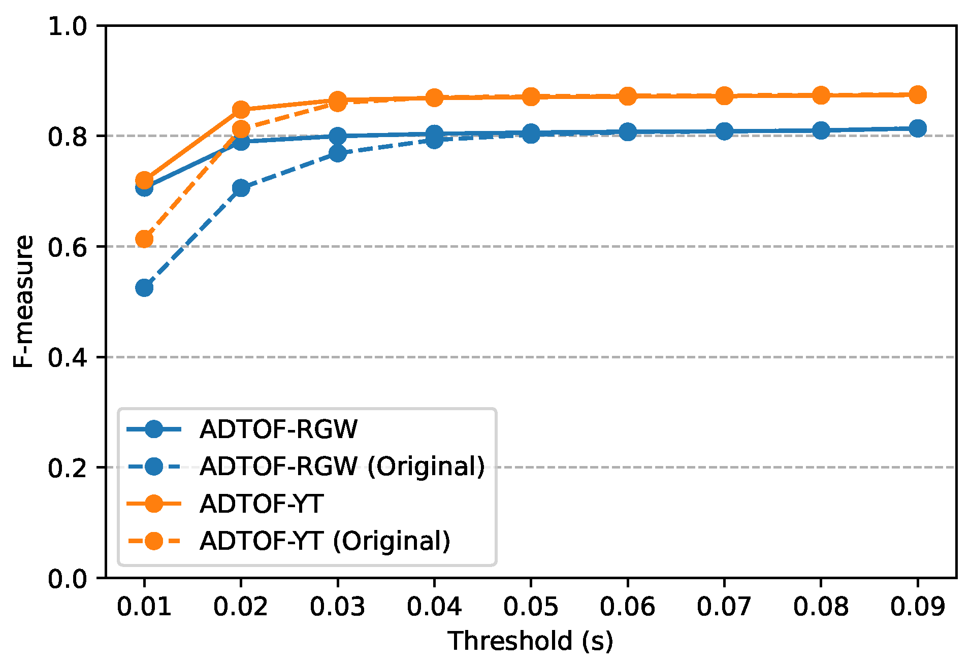
To evaluate each trained model, we compared its detected onsets to the ground-truth annotations independently for each dataset. The evaluation was based on the hit rate: An estimation was considered correct (a hit) if it was within 50 ms of an annotation, and all estimations and annotations were matched at most once (for the actual implementation, refer to the package mir_eval [37]). We counted the matched events as true positives (tp), the ground-truth annotations without a corresponding estimation as false negatives (fn), and the estimations not present in the ground-truth annotations as false positives (fp). Then, we computed the F-measure by summing the tp, fn, and fp across all tracks and all instruments in the test set of each dataset.

4.1. Evaluation of Architectures

Table 4. F-measure (between 0 and 1) for different architectures trained with all real-music datasets.

Architecture		ADTOF-RGW	ADTOF-YT	RBMA	ENST	MDB
Frame	RNN	0.83	0.85	0.65	0.78	0.81
	Self-att	0.83	0.85	0.64	0.79	0.79
Tatum	RNN	0.81	0.83	0.62	0.75	0.81
	Self-att	0.82	0.83	0.62	0.79	0.80

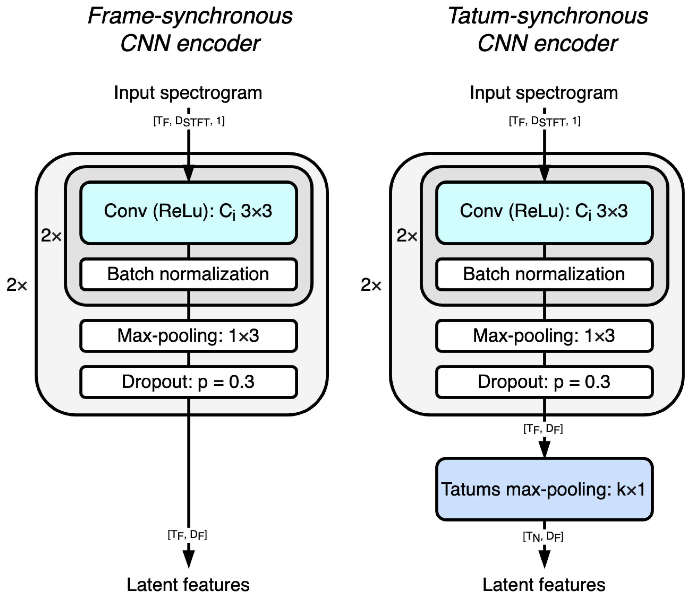
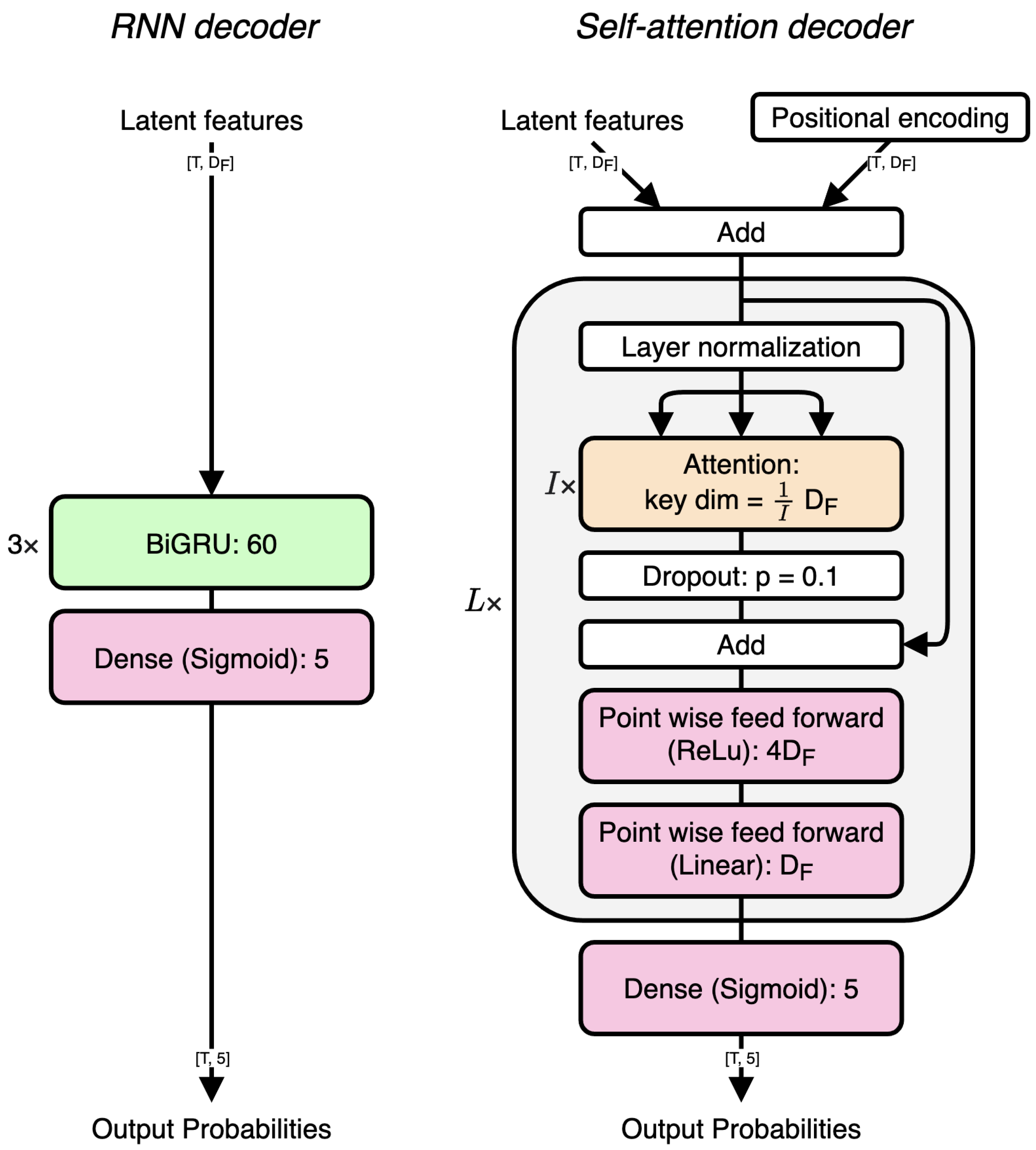
Values in bold are the best achieved on each dataset.

lists the four architectures we evaluated, specifically, a frame- or tatum-synchronous encoder, in combination with an RNN or self-attention decoder. In the following, we refer to the architecture consisting of the frame-synchronous encoder and RNN decoder as the “reference”.

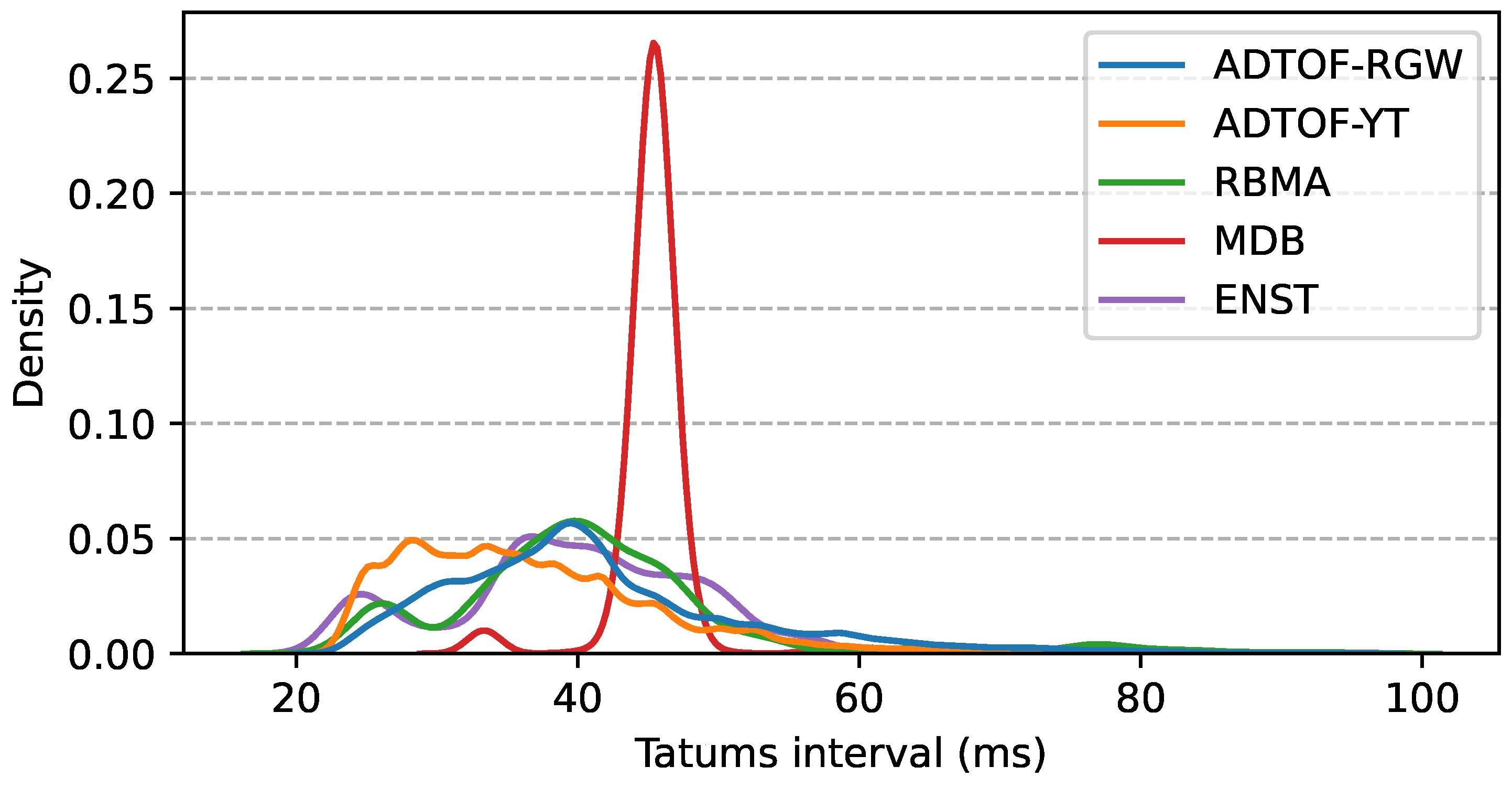
On average, the frame-synchronous models (top two rows in Table 4) performed slightly better than the tatum-synchronous models (bottom two rows). This empirical finding contrasts with both our intuition and the results of Ishizuka et al. [5,6], who observed that the tatum max-pooling layer always improved the F-measure achieved by the model. We hypothesize that the main reason behind the lower score for the tatum-synchronous models (compared to Ishizuka) lies in the lower quality of the tatum grid used for pooling. In fact, we computed an F-measure between Madmom and ground-truth beats of 0.71, 0.62, and 0.84 for ADTOF-RGW, ADTOF-YT, and RBMA, respectively, while Ishizuka et al. reported much higher scores of 0.93 and 0.96 on their two datasets. The disagreement between the estimated and annotated beats shows that the tatums we employed were likely based on erroneous beat positions, and this hindered the performance of the model.

By comparing the first two rows (frame-synchronous models) with one another, we conclude that the self-attention and RNN decoders obtained almost identical results. The same is true when comparing the third row with the fourth row (tatum-synchronous models). These results contrast with previous works, which tend to favor self-attention mechanisms over RNNs (see Table 1), especially in the presence of a large amount of training data, as in this study. An explanation is that the input sequence was short enough (4 s or 16 beats, T in Figure 2) to be fully modeled by an RNN, so no benefit was gained by employing the global sequence modeling capabilities of the self-attention mechanism.

While a finer hyperparameter search could slightly change the values presented in Table 4, the differences we observed among the four architectures were such that no clear winner emerged. Since neither the tatum synchronicity nor the self-attention mechanisms significantly improved the results, in the next experiment we focused on the simpler frame-synchronous RNN.

4.2. Evaluating Training Procedures

In the following, we evaluate the reference (frame-synchronous RNN) architecture when trained with nine different combinations of datasets. Specifically, we trained a model with and without specific datasets to measure (1) the contribution of the different datasets toward the model’s quality and (2) the generalization capabilities achieved on the datasets that were not used for the training. The results are presented in

Table 5. F-measure (between 0 and 1) for different training procedures achieved by the “frame RNN” architecture.

#	Training Dataset (s)		ADTOF-RGW	ADTOF-YT	RBMA	ENST	MDB
1		All five	0.83	0.85	0.65	0.78	0.81
2		ADTOF-RGW, ADTOF-YT	0.82	0.85	0.65	0.78	0.81
3		ADTOF-RGW (Zehren et al. [3])	0.79	0.73	0.63	0.72	0.76
4		ADTOF-YT	0.76	0.85	0.57	0.73	0.78
5		RBMA, ENST, MDB	0.63	0.48	0.57	0.73	0.74
6	pt TMIDT	All five	0.79	0.81	0.62	0.77	0.77
7		ADTOF-RGW, ADTOF-YT	0.79	0.81	0.62	0.76	0.77
8		RBMA, ENST, MDB (Vogl et al. [2])	0.70	0.56	0.63	0.76	0.75
9		-	0.70	0.62	0.60	0.75	0.68

Values in bold are the best achieved on each dataset. Zero-shot evaluations are highlighted in blue.

, where the top five rows refer to models trained without pre-training, while the bottom four rows refer to models that were pre-trained on the TMIDT dataset.

A comparison of the first two rows of Table 5 helps to understand the contribution (to the training) of the small non-crowdsourced datasets (RBMA, ENST, and MDB) when added to the crowdsourced data (ADTOF-RGW and YT). It can be observed that adding RBMA, ENST, and MDB to the training data did not improve the results of the model, except when testing on ADTOF-RGW, but only slightly (from 0.82 to 0.83). On the one hand, this reveals that the limited diversity of these datasets (RBMA, ENST, and MDB) prevented an improvement in the generalization of the model, even with the boosted sampling probability (Section 3.2). On the other hand, this also shows that the model trained exclusively on ADTOF-RGW and ADTOF-YT already performed well on other datasets (zero-shot performance of ADTOF-RGW plus ADTOF-YT on RBMA, ENST, and MDB).

By comparing rows 2 and 3, and rows 2 and 4, one can see the contribution of the datasets ADTOF-YT and ADTOF-RGW with respect to the training carried out using both. As expected, since these datasets are biased towards different music genres, their joint usage achieved noticeably better results for zero-shot performance. For instance, the addition of ADTOF-RGW to ADTOF-YT brought the F-score on RBMA from 0.57 to 0.65; likewise, the addition of ADTOF-YT to ADTOF-RGW brought the F-score on ENST and MDB from 0.72 and 0.76 to 0.78 and 0.81, respectively. In other words, since mixing these datasets increased the diversity of the training data, the zero-shot performance of the model also increased.

However, it is rather surprising to notice that while the addition of ADTOF-YT improved the performance on ADTOF-RGW (from 0.79 to 0.82), no improvement was observed on ADTOF-YT when ADTOF-RGW was added (the F-score stayed at 0.85). We attribute this behavior to the fact that ADTOF-RGW contains mistakes in the annotations and is smaller than ADTOF-YT. This effectively prevented the model trained exclusively on ADTOF-RGW from achieving the best performance on this dataset. Nonetheless, as already observed in [3], thanks to its large size and diversity, ADTOF-RGW was still better for training than any of the non-crowdsourced datasets (row 5).

Finally, we quantified the contribution of pre-training on the large synthetic dataset TMIDT, following a method suggested by Vogl et al. [2] and known to counter the data paucity of real-word recordings. We identified three trends with TMIDT: (i) Already before undergoing any refinement, the pre-trained model attained a performance (row 9) that on average outweighed that of the same model trained on RBMA, ENST, and MDB (row 5). This result, already identified by Vogl et al., is remarkable considering that during training the model was only exposed to synthesized data, i.e., data with limited acoustic diversity. (ii) When refining on RBMA, ENST, and MDB, the F-measure increased on these same datasets, but not on ADTOF-RGW nor ADTOF-YT (row 8). This is another indication that RBMA, ENST, and MDB did not contribute extensively to the quality of the models trained on them. (iii) Lastly, pre-training on TMIDT and then refining on ADTOF-RGW and ADTOF-YT yielded a lower F-measure than when no pre-training was performed (rows 6–7 compared to rows 1–2). This phenomenon, known as “ossification”, suggests that pre-training may have prevented the model from adapting to the fine-tuning distribution in the high data regime [38] (p. 7), that is, the model became stuck at a local minimum. Since pre-training did not help, this is an indication that ADTOF-RGW and ADTOF-YT likely contained enough (and diverse) data to train our model to its full potential.

We have so far discussed the results only for the reference architecture (frame- synchronous RNN). To ensure that the trends identified with the training data were not dependent on the architecture employed, we repeated the same evaluations with the frame-synchronous self-attention architecture, and we found scores that matched closely those in Table 5. We are thus confident that the trends we described hold in general. Nonetheless, we identified two key differences among the different architectures: First, when few data were available (i.e., when training exclusively on RBMA, ENST, and MDB), the model with the self-attention mechanism performed worse than when trained with the RNN. This matched the empirical results found by Ishizuka et al. [6], who claimed that the self-attention mechanism was affected more than the RNN by data size. Second, although pre-training on TMIDT still penalized the model through ossification, we noticed that the drop in performance was less significant with the self-attention mechanism than with the RNN. This occurred because the higher number of parameters in the self-attention architecture made it less prone to ossification, as Henandez suggested [38] (p. 7).

5. Conclusions

Given an input audio recording, we considered the task of automatically transcribing drums in the presence of melodic instruments. In this study, we introduced a new large crowdsourced dataset and addressed three issues related to the use of datasets of this type: the lack of investigations of deep learning architectures trained on them, the discrepancies and bias in crowdsourced annotations, and their limited evaluation.

Specifically, we first investigated four deep learning architectures that are well suited to leveraging large datasets. Starting from the well-known convolutional recurrent neural network (CRNN) architecture, we extended it to incorporate one or both of two mechanisms: tatum max-pooling and self-attention. We then mitigated discrepancies and bias in the training data by creating a new non-synthetic dataset (ADTOF-YT), which was significantly larger than other currently available datasets. ADTOF-YT was curated by gathering high-quality crowdsourced annotations, applying a cleansing procedure to make them compatible with the ADT task, and mixing it with other datasets to further diversify the training data. Finally, we evaluated many training procedures to quantify the contribution of each dataset to the performance of the model, in both zero-shot and non-zero-shot settings.

The results can be summarized as follows: (1) No noticeable difference was observed among the four architectures we tested. (2) The combination of the newly introduced dataset ADTOF-YT with the existing ADTOF-RGW proved to train models better than any previously used datasets, synthetic or not. (3) We quantified the generalization capabilities of the model when tested on unseen datasets and concluded that good generalization was achieved only when large amounts of crowdsourced data were included in the training procedure.

Thanks to this evaluation, we explored how to leverage crowdsourced datasets with different DL architectures and training scenarios. By achieving better results than the current state-of-the-art models, we improved the ability to retrieve information from music, be it for musicians who desire to learn a new musical piece, or for researchers who need to retrieve information from the location of the notes. Further, the models were approaching the Bayes error rate (irreducible error). In order to quantify the improvements that one can expect from a perfect classifier, in future work we aim to estimate this theoretical limit.

References

1. Wu, C.W.; Dittmar, C.; Southall, C.; Vogl, R.; Widmer, G.; Hockman, J.; Muller, M.; Lerch, A. A Review of Automatic Drum Transcription. IEEE/ACM Trans. Audio Speech Lang. Process. 2018, 26, 1457–1483. [Google Scholar] [CrossRef]
2. Vogl, R.; Widmer, G.; Knees, P. Towards multi-instrument drum transcription. In Proceedings of the 21th International Conference on Digital Audio Effects (DAFx-18), Aveiro, Portugal, 4–8 September 2018. [Google Scholar]
3. Zehren, M.; Alunno, M.; Bientinesi, P. ADTOF: A large dataset of non-synthetic music for automatic drum transcription. In Proceedings of the 22nd International Society for Music Information Retrieval Conference (ISMIR), Online, 7–12 November 2021; pp. 818–824. [Google Scholar]
4. Wei, I.C.; Wu, C.W.; Su, L. Improving Automatic Drum Transcription Using Large-Scale Audio-to-Midi Aligned Data. In Proceedings of the IEEE International Conference on Acoustics, Speech and Signal Processing (ICASSP), Toronto, ON, Canada, 6–11 June 2021; IEEE: Toronto, ON, Canada, 2021; pp. 246–250. [Google Scholar] [CrossRef]
5. Ishizuka, R.; Nishikimi, R.; Nakamura, E.; Yoshii, K. Tatum-Level Drum Transcription Based on a Convolutional Recurrent Neural Network with Language Model-Based Regularized Training. In Proceedings of the Asia-Pacific Signal and Information Processing Association Annual Summit and Conference (APSIPA ASC), Auckland, New Zealand, 7–10 December 2020; pp. 359–364. [Google Scholar]
6. Ishizuka, R.; Nishikimi, R.; Yoshii, K. Global Structure-Aware Drum Transcription Based on Self-Attention Mechanisms. Signals 2021, 2, 508–526. [Google Scholar] [CrossRef]
7. Vaswani, A.; Shazeer, N.; Parmar, N.; Uszkoreit, J.; Jones, L.; Gomez, A.N.; Kaiser, L.; Polosukhin, I. Attention Is All You Need. arXiv 2017, arXiv:1706.03762. [Google Scholar]
8. Jacques, C.; Roebel, A. Automatic drum transcription with convolutional neural networks. In Proceedings of the 21th International Conference on Digital Audio Effects (DAFx-18), Aveiro, Portugal, 4–8 September 2018; pp. 80–86. [Google Scholar]
9. Cartwright, M.; Bello, J.P. Increasing Drum Transcription Vocabulary Using Data Synthesis. In Proceedings of the 21th International Conference on Digital Audio Effects (DAFx-18), Aveiro, Portugal, 4–8 September 2018; pp. 72–79. [Google Scholar]
10. Choi, K.; Cho, K. Deep Unsupervised Drum Transcription. arXiv 2019, arXiv:1906.03697. [Google Scholar]
11. Jacques, C.; Roebel, A. Data Augmentation for Drum Transcription with Convolutional Neural Networks. arXiv 2019, arXiv:1903.01416. [Google Scholar]
12. Callender, L.; Hawthorne, C.; Engel, J. Improving Perceptual Quality of Drum Transcription with the Expanded Groove MIDI Dataset. arXiv 2020, arXiv:2004.00188. [Google Scholar]
13. Manilow, E.; Seetharaman, P.; Pardo, B. Simultaneous Separation and Transcription of Mixtures with Multiple Polyphonic and Percussive Instruments. In Proceedings of the IEEE International Conference on Acoustics, Speech and Signal Processing (ICASSP), Barcelona, Spain, 4–8 May 2020; IEEE: Barcelona, Spain, 2020; pp. 771–775. [Google Scholar] [CrossRef]
14. Wang, Y.; Salamon, J.; Cartwright, M.; Bryan, N.J.; Bello, J.P. Few-Shot Drum Transcription in Polyphonic Music. In Proceedings of the 21st International Society for Music Information Retrieval Conference (ISMIR), Montréal, QC, Canada, 11–15 October 2020; pp. 117–124. [Google Scholar]
15. Cheuk, K.W.; Herremans, D.; Su, L. ReconVAT: A Semi-Supervised Automatic Music Transcription Framework for Low-Resource Real-World Data. In Proceedings of the 29th ACM International Conference on Multimedia, Virtual Event, China, 20–24 October 2021; pp. 3918–3926. [Google Scholar] [CrossRef]
16. Gardner, J.; Simon, I.; Manilow, E.; Hawthorne, C.; Engel, J. MT3: Multi-Task Multitrack Music Transcription. In Proceedings of the International Conference on Learning Representations, Virtual, 3–7 May 2021; p. 21. [Google Scholar]
17. Simon, I.; Gardner, J.; Hawthorne, C.; Manilow, E.; Engel, J. Scaling Polyphonic Transcription with Mixtures of Monophonic Transcriptions. In Proceedings of the 23rd International Society for Music Information Retrieval Conference (ISMIR), Bengaluru, India, 4–8 December 2022; p. 8. [Google Scholar]
18. Cheuk, K.W.; Choi, K.; Kong, Q.; Li, B.; Won, M.; Hung, A.; Wang, J.C.; Herremans, D. Jointist: Joint Learning for Multi-instrument Transcription and Its Applications. arXiv 2022, arXiv:2206.10805. [Google Scholar]
19. Hennequin, R.; Khlif, A.; Voituret, F.; Moussallam, M. Spleeter: A fast and efficient music source separation tool with pre-trained models. J. Open Source Softw. 2020, 5, 2154. [Google Scholar] [CrossRef]
20. Manilow, E.; Wichern, G.; Seetharaman, P.; Le Roux, J. Cutting music source separation some Slakh: A dataset to study the impact of training data quality and quantity. In Proceedings of the IEEE Workshop on Applications of Signal Processing to Audio and Acoustics (WASPAA), New Paltz, NY, USA, 20–23 October 2019; IEEE: Piscataway, NJ, USA, 2019. [Google Scholar]
21. Ostermann, F.; Vatolkin, I.; Ebeling, M. AAM: A dataset of Artificial Audio Multitracks for diverse music information retrieval tasks. EURASIP J. Audio Speech Music. Process. 2023, 2023, 13. [Google Scholar] [CrossRef]
22. Raffel, C. Learning-Based Methods for Comparing Sequences, with Applications to Audio-to-MIDI Alignment and Matching; Columbia University: New York, NY, USA, 2016. [Google Scholar] [CrossRef]
23. Böck, S.; Korzeniowski, F.; Schlüter, J.; Krebs, F.; Widmer, G. madmom: A New Python Audio and Music Signal Processing Library. In Proceedings of the 24th ACM International Conference on Multimedia, Amsterdam, The Netherlands, 15–19 October 2016; pp. 1174–1178. [Google Scholar] [CrossRef]
24. Böck, S.; Krebs, F.; Widmer, G. Joint Beat and Downbeat Tracking with Recurrent Neural Networks. In Proceedings of the 17th International Society for Music Information Retrieval Conference (ISMIR), New York, NY, USA, 7–11 August 2016; pp. 255–261. [Google Scholar] [CrossRef]
25. Gillet, O.; Richard, G. ENST-Drums: An extensive audio-visual database for drum signals processing. In Proceedings of the 7th International Society for Music Information Retrieval Conference (ISMIR, Victoria, BC, Canada, 8–12 October 2006; pp. 156–159. [Google Scholar]
26. Southall, C.; Wu, C.W.; Lerch, A.; Hockman, J. MDB drums—An annotated subset of MedleyDB for Automatic Drum Transcription. In Proceedings of the 7th International Society for Music Information Retrieval Conference (ISMIR), Suzhou, China, 23–27 October 2017. [Google Scholar]
27. Vogl, R.; Dorfer, M.; Knees, P. Drum transcription from polyphonic music with recurrent neural networks. In Proceedings of the IEEE International Conference on Acoustics, Speech and Signal Processing (ICASSP), New Orleans, LA, USA, 5–9 March 2017; IEEE: New Orleans, LA, USA, 2017; pp. 201–205. [Google Scholar] [CrossRef]
28. Bittner, R.; Salamon, J.; Tierney, M.; Mauch, M.; Cannam, C.; Bello, J. MedleyDB: A multitrack dataset for annotation-intensive MIR research. In Proceedings of the 15th International Society for Music Information Retrieval Conference (ISMIR), Taipei, Taiwan, 27–31 October 2014; pp. 155–160. [Google Scholar]
29. Driedger, J.; Schreiber, H.; Bas de Haas, W.; Müller, M. Towards automatically correcting tapped beat annotations for music recordings. In Proceedings of the 20th International Society for Music Information Retrieval Conference (ISMIR), Delft, The Netherlands, 4–8 November 2019; pp. 200–207. [Google Scholar]
30. Xue, L.; Constant, N.; Roberts, A.; Kale, M.; Al-Rfou, R.; Siddhant, A.; Barua, A.; Raffel, C. mT5: A massively multilingual pre-trained text-to-text transformer. In Proceedings of the Conference of the North American Chapter of The Association for Computational Linguistics: Human Language Technologies, Online, 6–11 June 2021; pp. 483–498. [Google Scholar] [CrossRef]
31. Böck, S.; Davies, M.E.P. Deconstruct, Analyse, Reconstruct: How to improve Tempo, Beat, and Downbeat Estimation. In Proceedings of the 21st International Society for Music Information Retrieval Conference (ISMIR), Montréal, QC, Canada, 11–15 October 2020; pp. 574–582. [Google Scholar]
32. Hung, Y.N.; Wang, J.C.; Song, X.; Lu, W.T.; Won, M. Modeling Beats and Downbeats with a Time-Frequency Transformer. In Proceedings of the IEEE International Conference on Acoustics, Speech and Signal Processing (ICASSP), Singapore, 23–27 May 2022; pp. 401–405. [Google Scholar] [CrossRef]
33. Pedregosa, F.; Varoquaux, G.; Gramfort, A.; Michel, V.; Thirion, B.; Grisel, O.; Blondel, M.; Prettenhofer, P.; Weiss, R.; Dubourg, V.; et al. Scikit-learn: Machine learning in Python. J. Mach. Learn. Res. 2011, 12, 2825–2830. [Google Scholar]
34. Kingma, D.P.; Ba, J. Adam: A Method for Stochastic Optimization. arXiv 2017, arXiv:1412.6980. [Google Scholar]
35. Abadi, M.; Agarwal, A.; Barham, P.; Brevdo, E.; Chen, Z.; Citro, C.; Corrado, G.S.; Davis, A.; Dean, J.; Devin, M.; et al. TensorFlow: Large-scale machine learning on heterogeneous systems. arXiv 2016, arXiv:1603.04467. [Google Scholar]
36. Raffel, C.; Ellis, D.P.W. Intuitive Analysis, Creation and Manipulation of MIDI Data with pretty_midi. In Proceedings of the 15th International Society for Music Information Retrieval Conference, Taipei, Taiwan, 27–31 October 2014. [Google Scholar]
37. Raffel, C.; McFee, B.; Humphrey, E.J.; Salamon, J.; Nieto, O.; Liang, D.; Ellis, D.P.W. mir_eval: A transparent implementation of common MIR metrics. In Proceedings of the 15th International Society for Music Information Retrieval Conference (ISMIR), Taipei, Taiwan, 27–31 October 2014; pp. 367–372. [Google Scholar]
38. Hernandez, D.; Kaplan, J.; Henighan, T.; McCandlish, S. Scaling Laws for Transfer. arXiv 2021, arXiv:2102.01293. [Google Scholar]
39. Rolnick, D.; Veit, A.; Belongie, S.; Shavit, N. Deep Learning is Robust to Massive Label Noise. arXiv 2018, arXiv:1705.10694. [Google Scholar]
40. Nieto, O.; McCallum, M.; Davies, M.E.P.; Robertson, A.; Stark, A.; Egozy, E. The Harmonix Set: Beats, Downbeats, and Functional Segment Annotations of Western Popular Music. In Proceedings of the 20th International Society for Music Information Retrieval Conference (ISMIR), Delft, The Netherlands, 4–8 November 2019; pp. 565–572. [Google Scholar]
Figure 1. Detailed architecture for the frame-synchronous CNN encoder (left) and the tatum-synchronous CNN encoder (right). Each architecture has two stacks of two convolutional layers (cyan) with batch normalization, followed by max-pooling and dropout layers. Tatum synchronicity is achieved with max-pooling on the frame dimension (blue).
Signals 04 00042 g001
Figure 2. Detailed architecture for the RNN decoder (left) and the self-attention decoder (right). In summary, the RNN consists of three layers of bi-directional gated recurrent units (green). The self-attention mechanism consists of L stacks of multi-head self-attention (orange).
Signals 04 00042 g002
Figure 3. A beat divided into 12 even intervals accommodates 16th notes and 16th-note triplets.
Signals 04 00042 g003
Figure 4. Distribution of the tatum intervals, derived from Madmom’s beats subdivided 12 times, for each dataset.
Signals 04 00042 g004
Figure 5. Genre distribution for both ADTOF datasets.
Signals 04 00042 g005