Radix-2² Algorithm for the Odd New Mersenne Number Transform (ONMNT)

Abstract

This paper introduces a new derivation of the radix-$2^2$ fast algorithm for the forward odd new Mersenne number transform (ONMNT) and the inverse odd new Mersenne number transform (IONMNT). This involves introducing new equations and functions in finite fields, bringing particular challenges unlike those in other fields. The radix-$2^2$ algorithm combines the benefits of the reduced number of operations of the radix-4 algorithm and the simple butterfly structure of the radix-2 algorithm, making it suitable for various applications such as lightweight ciphers, authenticated encryption, hash functions, signal processing, and convolution calculations. The multidimensional linear index mapping technique is the conventional method used to derive the radix-$2^2$ algorithm. However, this method does not provide clear insights into the underlying structure and flexibility of the radix-$2^2$ approach. This paper addresses this limitation and proposes a derivation based on bit-unscrambling techniques, which reverse the ordering of the output sequence, resulting in efficient calculations with fewer operations. Butterfly and signal flow diagrams are also presented to illustrate the structure of the fast algorithm for both ONMNT and IONMNT. The proposed method should pave the way for efficient and flexible implementation of ONMNT and IONMNT in applications such as lightweight ciphers and signal processing. The algorithm has been implemented in C and is validated with an example.

1. Introduction

Number theoretic transforms (NTTs) [1] have many applications [2] in signal processing and cryptography [1]. Two well-known NTTs are the Mersenne number transform (MNT) [3,4] and the Fermat number transform (FNT) [5,6], which are based on Mersenne numbers and Fermat numbers, respectively. MNT has been given particular attention as it has simple arithmetic and favorable reduction operations compared to FNT. However, MNT has limitations in terms of its transform length, which is short and has limited factorability, making it unfeasible to use the fast algorithm.

To address the limitations of MNT, Bousssakta and Holt introduced the new Mersenne number transform (NMNT) [7]. Later, two new variants named the odd new Mersenne number transform (ONMNT) and the odd square new Mersenne number transform (O²NMNT) were proposed; these are known as generalized new Mersenne number transforms (GNMNTs) [8]. These two transforms have shown promising results in signal processing, image processing, and cryptography [9]. Parameterized implementation, strong diffusion performance, and simple arithmetic operations are critical advantages of NMNT-based cryptographic ciphers over conventional ciphers.

One of the advantages of the NMNT family of transforms is their suitability for fast algorithms, as their transform length is always a power of 2. A detailed discussion on different fast algorithms such as radix-2, radix-4, and split-radix for NMNT and GNMNT can be found in [9,10]. Hue et al. [11] presented a realization of NMNT using the Walsh–Hadamard Transform (WHT) to speed up the calculation. The split-radix algorithm has the lowest arithmetic complexity. It avoids the limitation of the radix-4 algorithm, which can only be applied for a transform length N with an odd power of 4. However, the structure of the split-radix algorithm is highly complex, and its implementation in a simple hardware system is challenging. A new class of fast algorithms called radix-$2^2$ [12] algorithms has been proposed, incorporating a twiddle factor decomposition technique in an efficient divide and conquer method, which leads to a regular signal flow graph structure. The structure of the radix is a crucial factor in determining the architecture of the fast Fourier transform (FFT) [13] processor. A simple and regular radix structure allows for an efficient implementation of the architecture [14]. The radix-$2^2$ algorithm retains both the low multiplicative complexity of the radix-4 algorithm and the simple structure of the radix-2 algorithm. Thus, it solves both these limitations. This algorithm can be used directly for even values of n, where $N=2^n$, and for odd values of n simply by utilizing a mixed-radix algorithm at the beginning or end of the radix-$2^2$ algorithm. The radix-$2^2$ algorithm can, therefore, be implemented for any value of N that is a power of 2. Moreover, significant memory savings have been achieved using this algorithm [15]. Therefore, multiple efficient implementations of the radix-$2^2$ FFT algorithm have been proposed for application-specific integrated circuits (ASIC) [16] and field-programmable gate arrays (FPGA) [16,17,18], primarily in the field of wireless communication.

Lightweight cryptography [19] is another area of research that can benefit from the efficient implementation of radix-$2^2$ algorithms in resource-constrained devices, such as in radio frequency identification (RFID), sensors, wireless Internet of Things (IoT) devices [20], smart home automation, telemedicine, smart money [21], healthcare, and military applications. Efficient hardware implementations [22] are important in lightweight cryptography. In recent years, number theoretic transform-based cryptographic systems have been proposed, especially for the IoT [23,24,25]. One of the advantages of number theoretic transforms such as ONMNT is the ability to use fast algorithms. As the radix-$2^2$ fast algorithm offers a simple butterfly structure while maintaining the multiplicative complexity of the radix-4 algorithm, the derivation of the radix-$2^2$ fast algorithm for ONMNT will improve the efficiency for ONMNT-based lightweight ciphers. In the literature, there are two main approaches to implementing the radix-$2^2$ algorithm. The first approach is based on multidimensional index mapping [26], while the second is the twiddle factor unscrambling technique [27]. In conventional multidimensional index mapping, the transform length N is mapped onto a multidimensional array, following a similar approach to the Cooley–Tukey algorithm. In the twiddle factor unscrambling technique [28], the segment is divided into $N/4$ equal segments, and each smaller butterfly is rearranged to be in base 2 or bit-reversed order rather than in base 4 or in word-reversed order, which is typical for the general radix-4 algorithm. This technique is comparatively efficient, and in this paper, we use the twiddle factor unscrambling technique to derive a radix-$2^2$ algorithm for ONMNT. The benefit of using the bit-unscrambling technique is that a higher-order radix, such as 4, 8, 16 or $2^i$, can use the same bit-unscrambling counter, which speeds up the calculation [29] without needing extra calculations and data processing. This fast algorithm can be used in a lightweight cipher, in which reducing the number of operations leads to a compact implementation and efficient convolution calculations in signal processing applications. In [30], the authors presented promising results on using the bit-unscrambling technique for radix $2^2$. It showed the dual advantages of a simpler structure and a reduced number of calculations. However, the paper was limited to NMNT. ONMNT is a more recent GNMNT, and it offers strong diffusion performance [9]. Unlike NMNT and O²NMNT, the kernel matrix for ONMNT is transposed in the inverse transform. Moreover, the derivation of the ONMNT fast algorithm requires considering retrograde points. Fast algorithms for ONMNT using radix $2^2$ have not been explored yet. Therefore, the aim of this paper is to develop the radix-$2^2$ fast algorithm for the calculation of the ONMNMT and IONMNT.

The original contributions of this paper are as follows:

• A novel mathematical derivation of a radix-$2^2$ algorithm for ONMNT and the inverse ONMNT (IONMNT) using the radix-$2^2$ bit-unscrambling technique.
• A detailed derivation of the transform kernel relationships incorporating retrograde points.
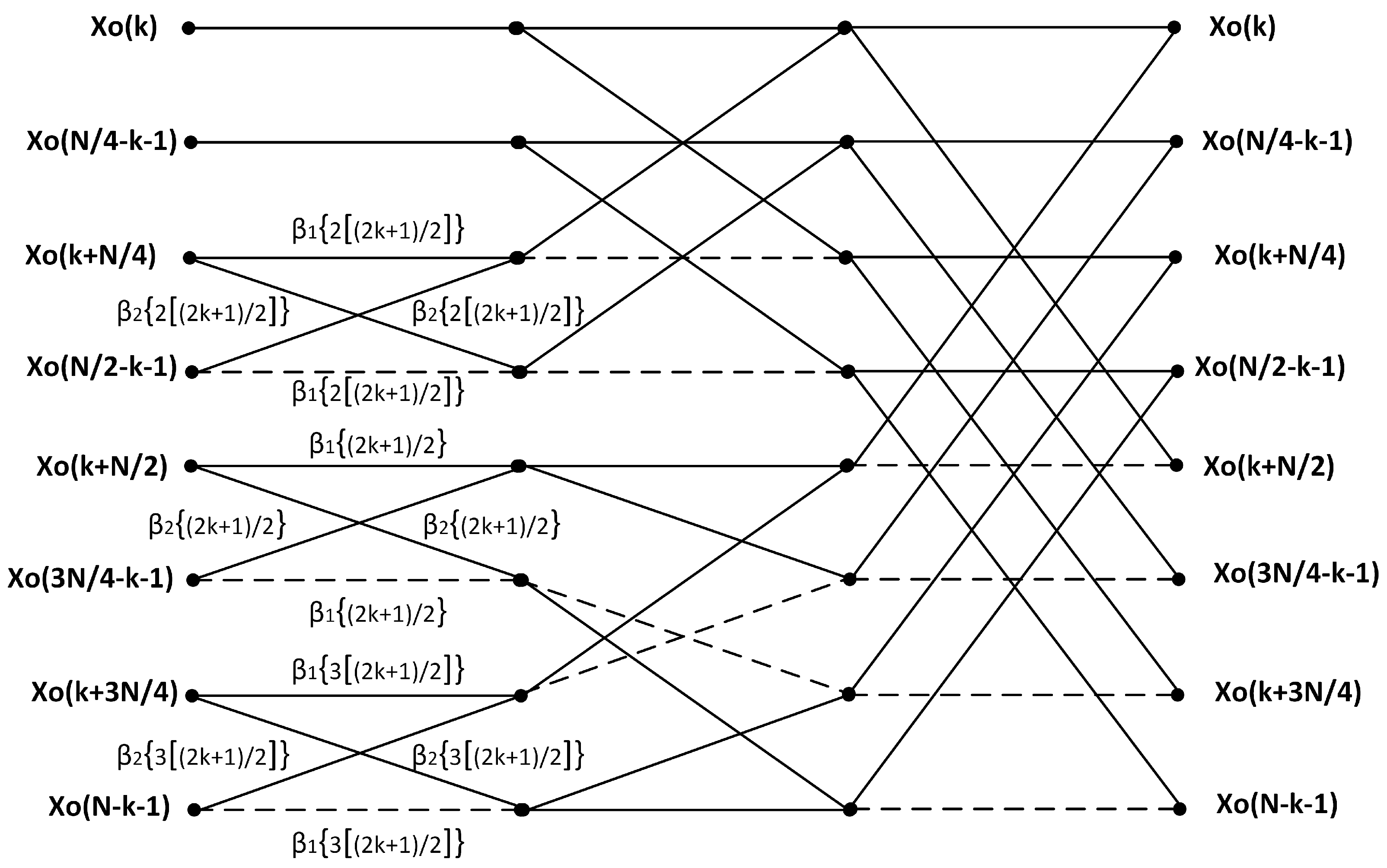
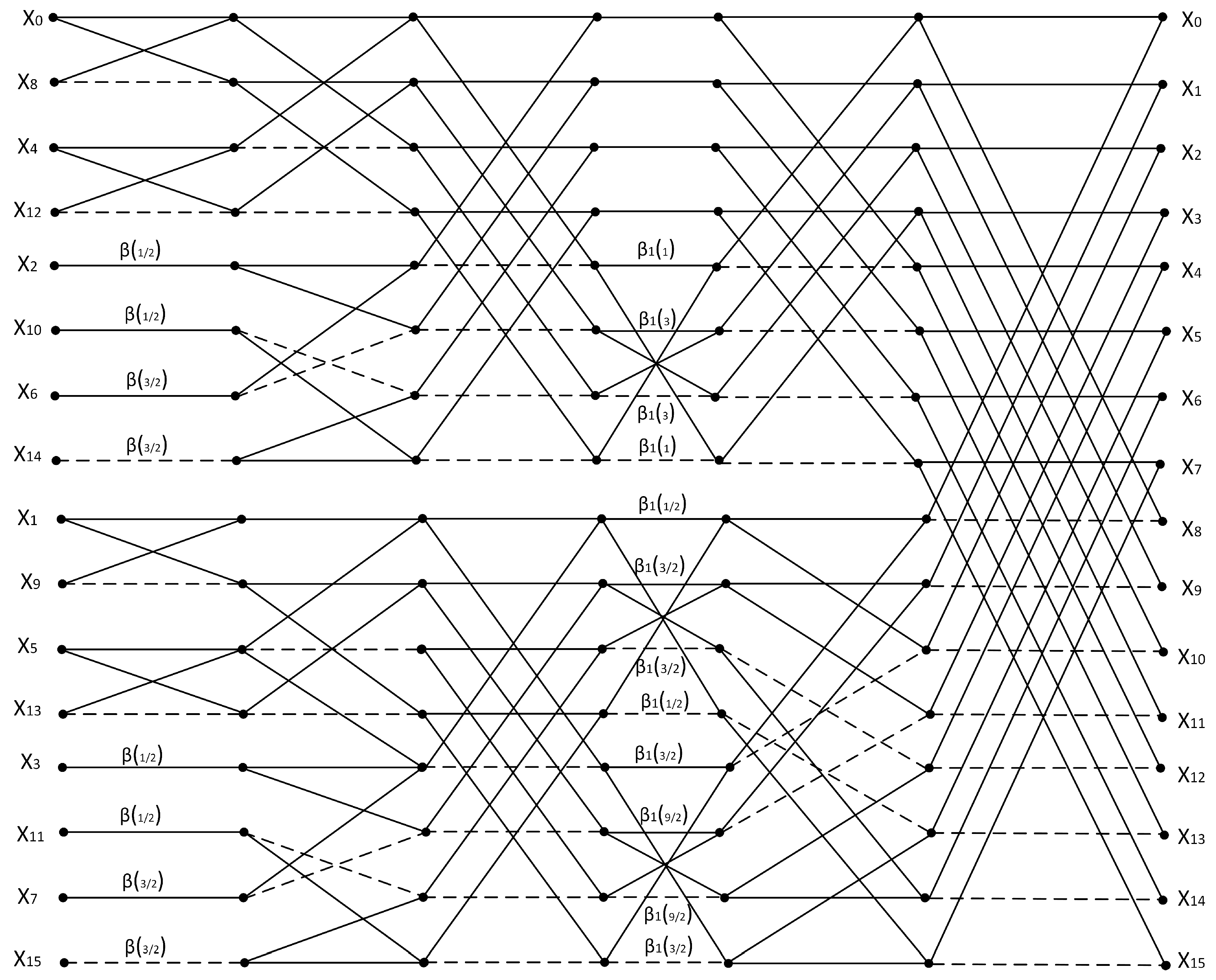
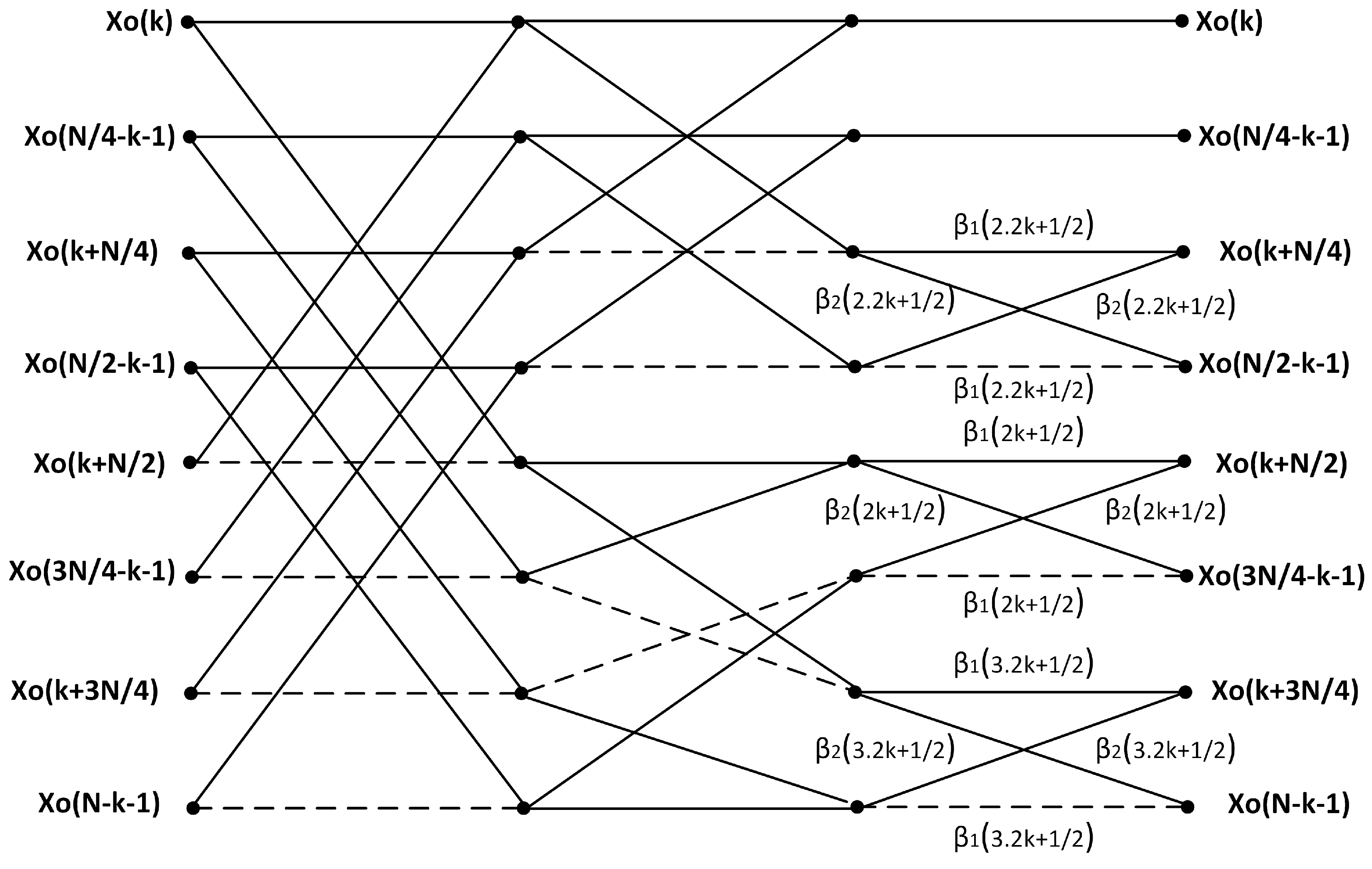
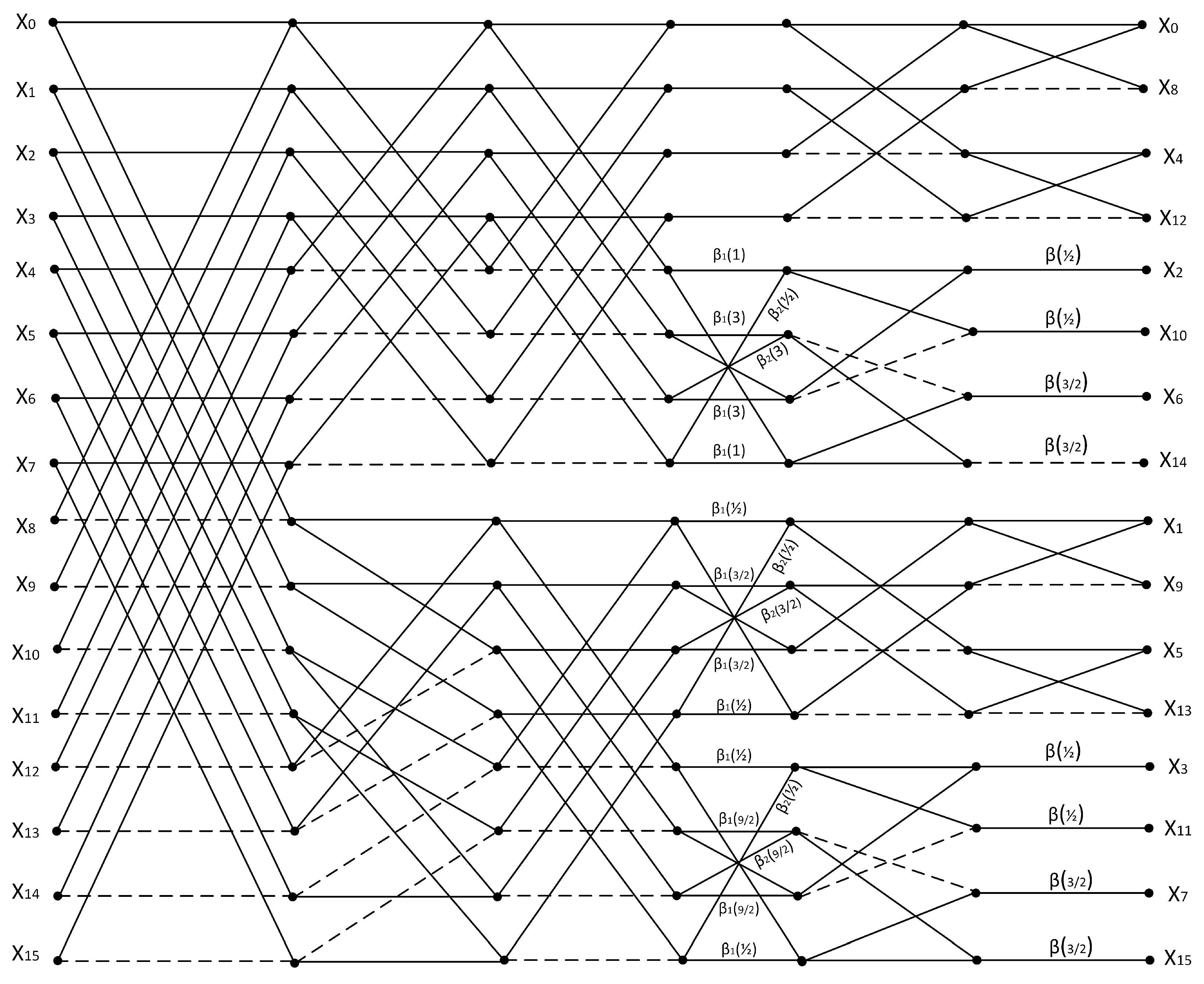
• Butterfly diagrams and signal flow graphs of the Radix-$2^2$ algorithm for ONMNT and IONMNT.

Regarding the rest of the paper, Section 2 describes the most common fast algorithms. Section 3 and Section 4 provide a detailed derivation of the radix-$2^2$ algorithm for the forward and inverse ONMNT with a butterfly diagram and a signal flow diagram, respectively. Section 5 discusses the arithmetic complexity of the proposed fast algorithm and compares it with direct calculation and radix-$2^2$. Section 6 presents an example to demonstrate the accuracy of the proposed fast algorithm. Section 7 concludes the paper and provides suggestions for future work.

2. Odd New Mersenne Number Transform

ONMNT is the first of the two new NMNT-based transforms introduced by Boussakta et al. [8]. An odd member of the transform parameter is chosen to form the kernel matrix.

The ONMNT of an integer sequence $x\left(n\right)$, where $n=0,1,2,3,\cdots ,N-1$ with transform length $N=2^m$ for $m=1,2,3,\cdots ,p-1$, is defined as follows:

$$X_o\left(k\right)={〈\sum _{n=0}^{N-1}x\left(n\right)\beta \left(\frac{n(2k+1)}{2}\right)〉}_{M_p}$$

(1)

where $k=0,1,2,\cdots ,N-1$, ${\langle .\rangle }_{M_p}$ represents modulo $M_p$ where $M_p=2^p-1$ is a Mersenne prime for $p=2,3,5,7,13,17,19,\cdots$ and $\beta \left(\frac{n(2k+1)}{2}\right)$ is the transform kernel. For the ONMNT, the transform kernel can be expressed by the following matrix:

$$M_{o_f}=\left[\begin{array}{cccc}\beta \left(0\right)& \beta \left(0\right)& \cdots & \beta \left(0\right)\\ \beta \left(\frac{1}{2}\right)& \beta \left(\frac{3}{2}\right)& \cdots & \beta \left(\frac{2N-1}{2}\right)\\ \beta \left(1\right)& \beta \left(3\right)& \cdots & \beta \left(2(N-1)\right)\\ \beta \left(\frac{3}{2}\right)& \beta \left(\frac{9}{2}\right)& \cdots & \beta \left\{\frac{3(2N-1)}{2}\right\}\\ ⋮& ⋮& \ddots & ⋮\\ \beta \left(\frac{N-1}{2}\right)& \beta \left\{\frac{3(N-1)}{2}\right\}& \cdots & \beta \left\{\frac{(2N-1)(N-1)}{2}\right\}\end{array}\right]$$

(2)

The IONMNT is defined as follows:

$$x\left(n\right)={〈N^{-1}\sum _{k=0}^{N-1}{X}_0\left(k\right)\beta \left(k\frac{2n+1}{2}\right)〉}_{M_p}$$

(3)

where $n=0,1,2,3,\cdots ,N-1$, $X_0\left(k\right)$ is the input sequence and $\beta \left(k\frac{2n+1}{2}\right)$ is the kernel parameter for IONMNT. When comparing (1) and (3), the IONMNT differs from the ONMNT in two ways: it has a scaling factor $N^{-1}$ and the transform matrix is transposed (i.e., $M_{o_i}=M_{o_f}^T$) to let the kernel matrix be orthogonal. Therefore, the following is the kernel matrix of the inverse ONMNT:

$$M_{o_i}=\left[\begin{array}{cccc}\beta \left(0\right)& \beta \left(\frac{1}{2}\right)& \cdots & \beta \left(\frac{N-1}{2}\right)\\ \beta \left(0\right)& \beta \left(\frac{3}{2}\right)& \cdots & \beta \left\{\frac{3(N-1)}{2}\right\}\\ \beta \left(0\right)& \beta \left(\frac{5}{2}\right)& \cdots & \beta \left\{\frac{5(2N-1)}{2}\right\}\\ ⋮& ⋮& \ddots & ⋮\\ \beta \left(0\right)& \beta \left(\frac{2N-1}{2}\right)& \cdots & \beta \left\{\frac{(N-1)(2N-1)}{2}\right\}\end{array}\right]$$

(4)

The maximum transform length for ONMNT is $N_{\max }=2^{p-1}$.

3. Derivation of Radix-${\mathbf{2}}^{\mathbf{2}}$ Algorithm for ONMNT

An ONMNT radix-$2^2$ algorithm can be developed by decomposing (1) into $2^2=4$ equal partial sums of transform length $\frac{N}{4}$, where $n=0,1,2,\cdots \frac{N}{4}-1$, and by replacing n with $4n+l$, where $l=0,1,2,\cdots \frac{N}{4}-1$. Therefore, (1) can be written as follows:

$$X^o\left(k\right)={〈\sum _{l=0}^3\sum _{n=0}^{N-1}x(4n+l).\beta \left((4n+l)\frac{2k+1}{2}\right)〉}_{M_p}$$

(5)

where $x(4n+l)$ is the input sequence of each segment, $\beta \left((4n+l)\frac{2k+1}{2}\right)$ is the kernel parameter of ONMNT and ${\langle .\rangle }_{M_p}$ means that the calculation is modulo a Mersenne prime. From the above equation, it can be seen that the output $X^o\left(k\right)$ of the ONMNT is the summation of four equal segments $X^o\left(k+\lambda \frac{N}{4}\right)$ with $\frac{N}{4}$ consecutive elements indexed by $\lambda$ and where $0\le \lambda \le 3$. A general equation for each partial sum or segment is

$$X^o\left(k+\lambda \frac{N}{4}\right)={〈\sum _{l=0}^3\sum _{n=0}^{\frac{N}{4}-1}x(4n+l)\beta \left\{(4n+l)\left(\frac{2k+1}{2}+\lambda \frac{N}{4}\right)\right\}〉}_{M_p}.$$

(6)

In the next step of the derivation, the twiddle factor, $\beta (.)$ from (3), is simplified as follows:

$$\beta \left\{(4n+l)\left(\frac{2k+1}{2}+\lambda \frac{N}{4}\right)\right\}=\beta \left[\left\{\left(\frac{2k+1}{2}\right)l+\lambda l\frac{N}{4}\right\}+\left\{4n\left(\frac{2k+1}{2}\right)+\lambda nN\right\}\right].$$

(7)

Equation (7) can be expanded using the $\beta$ properties of $\beta (m+n)={\beta }_1\left(m\right)\beta \left(n\right)+{\beta }_2\left(m\right)\beta (-n)$ from [31] as follows:

$$\begin{array}{c}\beta \left[\left\{\left(\frac{2k+1}{2}\right)l+\lambda l\frac{N}{4}\right\}+\left\{4n\left(\frac{2k+1}{2}\right)+\lambda nN\right\}\right]\hfill \\ \hspace{0.5em}\hspace{0.5em}\hspace{0.5em}\hspace{0.5em}={\beta }_1\left\{\left(\frac{2k+1}{2}\right)l+\lambda l\frac{N}{4}\right\}\beta \left\{4n\left(\frac{2k+1}{2}\right)+\lambda nN\right\}\\ \hfill \hspace{0.5em}\hspace{0.5em}\hspace{0.5em}\hspace{0.5em}\hspace{0.5em}\hspace{0.5em}\hspace{0.5em}\hspace{0.5em}\hspace{0.5em}\hspace{0.5em}\hspace{0.5em}\hspace{0.5em}\hspace{0.5em}\hspace{0.5em}\hspace{0.5em}+{\beta }_2\left\{\left(\frac{2k+1}{2}\right)l+\lambda l\frac{N}{4}\right\}\beta \left\{-4n\left(\frac{2k+1}{2}\right)+\lambda nN\right)\}\end{array}$$

(8)

where, using the periodic property of $\beta \left(n\right)$, i.e., $\beta (aN+m)=\beta \left(m\right)$ [30], (8) can be written as follows:

$$\begin{array}{c}\beta \left[\left\{\left(\frac{2k+1}{2}\right)l+\lambda l\frac{N}{4}\right\}+\left\{4n\left(\frac{2k+1}{2}\right)+\lambda nN\right\}\right]\hfill \\ \hspace{1em}\hspace{1em}\hspace{1em}\hspace{1em}\hspace{1em}\hspace{1em}\hspace{1em}={\beta }_1\left\{\left(\frac{2k+1}{2}\right)l+\lambda l\frac{N}{4}\right\}\beta \left\{4n\left(\frac{2k+1}{2}\right)\right\}\hfill \\ \hspace{1em}\hspace{1em}\hspace{1em}\hspace{1em}\hspace{1em}\hspace{1em}\hspace{1em}\hspace{1em}\hspace{1em}\hspace{1em}\hspace{1em}\hspace{1em}\hspace{1em}+{\beta }_2\left\{\left(\frac{2k+1}{2}\right)l+\lambda l\frac{N}{4}\right\}\beta \left\{-4n\left(\frac{2k+1}{2}\right)\right\}.\hfill \end{array}$$

(9)

Substituting ${\beta }_1(.)$ and ${\beta }_2(.)$ with the relations ${\beta }_1(m+n)={\beta }_1\left(m\right){\beta }_1\left(n\right)-{\beta }_2\left(m\right){\beta }_2\left(n\right)$ and ${\beta }_2(m+n)={\beta }_1\left(m\right){\beta }_2\left(n\right)+{\beta }_2\left(m\right){\beta }_1\left(n\right)$ from (9) into (7) yields the following:

$$\begin{array}{c}\beta \left\{(4n+l)\left(\frac{2k+1}{2}+\lambda \frac{N}{4}\right)\right\}=\left[{\beta }_1\left\{\left(\frac{2k+1}{2}\right)l\right\}{\beta }_1\left(\lambda l\frac{N}{4}\right)-{\beta }_2\left\{\left(\frac{2k+1}{2}\right)l\right\}{\beta }_2\left(\lambda l\frac{N}{4}\right)\right]\beta \left\{4n\frac{2k+1}{2}\right\}\hspace{0.5em}\hspace{0.5em}\hspace{0.5em}\hfill \\ \hfill +\left[{\beta }_1\left\{\left(\frac{2k+1}{2}\right)l\right\}{\beta }_2\left(\lambda l\frac{N}{4}\right)+{\beta }_2\left\{\left(\frac{2k+1}{2}\right)l\right\}{\beta }_1\left(\lambda l\frac{N}{4}\right)\right]\beta \left\{-4n\frac{2k+1}{2}\right\}.\end{array}$$

(10)

Substituting the values from (10) into (3), ignoring the modulo operator ${\langle \rangle }_{M_p}$ and rearranging yields

$$\begin{array}{cc}\hfill X^o\left(k+\lambda \frac{N}{4}\right)=\sum _{l=0}^3[& [\sum _{n=0}^{\frac{N}{4}-1}x(4n+l)\beta \left\{4n\left(\frac{2k+1}{2}\right)\right\}{\beta }_1\left(\lambda l\frac{N}{4}\right)\hfill \\ & +\sum _{n=0}^{\frac{N}{4}-1}x(4n+l)\beta \left\{4n\frac{2k+1}{2}\right\}{\beta }_2\left(\lambda l\frac{N}{4}\right)]{\beta }_1\left\{\left(\frac{2k+1}{2}\right)l\right\}\hfill \\ & +[\sum _{n=0}^{\frac{N}{4}-1}x(4n+l)\beta \left\{-4n\left(\frac{2k+1}{2}\right)\right\}{\beta }_1\left(\lambda l\frac{N}{4}\right)\hfill \\ & -\sum _{n=0}^{\frac{N}{4}-1}x(4n+l)\beta \left\{-4n\left(\frac{2k+1}{2}\right)\right\}{\beta }_2\left(\lambda l\frac{N}{4}\right)\left]{\beta }_2\left\{\left(\frac{2k+1}{2}\right)l\right\}\right]\hfill \end{array}$$

(11)

The following two sequences, where $l=0,1,2$ and 3, can be defined:

$$\begin{array}{c}{X}_l^o\left(k\right)=\sum _{n=0}^{\frac{N}{4}-1}x(4n+l)\beta \left\{4n\left(\frac{2k+1}{2}\right)\right\},\end{array}$$

(12)

$$\begin{array}{c}{X}_l^o\left(\frac{N}{4}-k-1\right)=\sum _{n=0}^{\frac{N}{4}-1}x(4n+l)\beta \left\{-4n\left(\frac{2k+1}{2}\right)\right\}.\end{array}$$

(13)

Substituting $X_l^o\left(k\right)$ and $X_l^o\left(\frac{N}{4}-k-1\right)$ from (12) and (13) into (11), and rearranging and applying re-indexing l of ${\beta }_1\left(\frac{2k+1}{2}l\right)$ and ${\beta }_2\left(\frac{2k+1}{2}l\right)$ from (11) according to the bit reverse order, yields the following:

$$\begin{array}{cc}\hfill X^o\left(k+\lambda \frac{N}{4}\right)=& X_0^o\left(k\right)\hfill \\ \hfill +& \left\{X_1^o\left(k\right){\beta }_1\left(\lambda \frac{N}{4}\right)+X_1^o\left(\frac{N}{4}-k-1\right){\beta }_2\left(\lambda \frac{N}{4}\right)\right\}{\beta }_1\left(2\frac{2k+1}{2}\right)\hfill \\ \hfill +& \left\{X_1^o\left(\frac{N}{4}-k-1\right){\beta }_1\left(\lambda \frac{N}{4}\right)-X_1^o\left(k\right){\beta }_2\left(\lambda \frac{N}{4}\right)\right\}{\beta }_2\left(2\frac{2k+1}{2}\right)\hfill \\ \hfill +& \left\{X_2^o\left(k\right){\beta }_1\left(\lambda \frac{N}{2}\right)+X_2^o\left(\frac{N}{4}-k-1\right){\beta }_2\left(\lambda \frac{N}{2}\right)\right\}{\beta }_1\left(\frac{2k+1}{2}\right)\hfill \\ \hfill +& \left\{X_2^o\left(\frac{N}{4}-k-1\right){\beta }_1\left(\lambda \frac{N}{2}\right)-X_2^o\left(k\right){\beta }_2\left(\lambda \frac{N}{2}\right)\right\}{\beta }_2\left(\frac{2k+1}{2}\right)\hfill \\ \hfill +& \left\{X_3^o\left(k\right){\beta }_1\left(\lambda \frac{3N}{4}\right)+X_3^o\left(\frac{N}{4}-k-1\right){\beta }_2\left(\lambda \frac{3N}{4}\right)\right\}{\beta }_1\left(3\frac{2k+1}{2}\right)\hfill \\ \hfill +& \left\{X_3^o\left(\frac{N}{4}-k-1\right){\beta }_1\left(\lambda \frac{3N}{4}\right)-X_3^o\left(k\right){\beta }_2\left(\lambda \frac{3N}{4}\right)\right\}{\beta }_2\left(3\frac{2k+1}{2}\right).\hfill \end{array}$$

(14)

Equation (14) is the general decomposition equation. The four main points for radix $2^2$ are $X^o\left(k\right)$, $X^o\left(k+\frac{N}{4}\right)$, $X^o\left(k+\frac{N}{2}\right)$ and $X^o\left(k+\frac{3N}{4}\right)$, which are derived by setting $\lambda =0,1,2,3$ in (14) and using the following beta relationships:

$${\beta }_1\left(0\right)=1$$

(15)

$${\beta }_2\left(0\right)=0$$

(16)

$${\beta }_1\left(a\frac{N}{4}\right)=\left\{\begin{array}{cc}{(-1)}^{\frac{a}{2}},\hfill & a\mathrm{is}\mathrm{even}\hfill \\ 0,\hfill & a\mathrm{is}\mathrm{odd}\hfill \end{array}\right.$$

(17)

$${\beta }_2\left(a\frac{N}{4}\right)=\left\{\begin{array}{cc}0,\hfill & a\mathrm{is}\mathrm{even}\hfill \\ {(-1)}^{\frac{a-1}{2}},\hfill & a\mathrm{is}\mathrm{odd}\hfill \end{array}\right.$$

(18)

$${\beta }_1\left(a\frac{N}{2}\right)={(-1)}^a$$

(19)

$${\beta }_2\left(a\frac{N}{2}\right)=0.$$

(20)

Then, the following mapping relations are applied:

$$X_0^o\left(k\right)=X^o\left(k\right)$$

(21)

$$X_1^o\left(k\right)=X^o\left(k+\frac{N}{4}\right)$$

(22)

$$X_1^o\left(\frac{N}{4}-k-1\right)=X^o\left(\frac{N}{2}-k-1\right)$$

(23)

$$X_2^o\left(k\right)=X^o\left(k+\frac{N}{2}\right)$$

(24)

$$X_2^o\left(\frac{N}{4}-k-1\right)=X^o\left(\frac{3N}{4}-k-1\right)$$

(25)

$$X_3^o\left(k\right)=X^o\left(k+\frac{3N}{4}\right)$$

(26)

$$X_3^o\left(k\right)=X^o\left(N-k-1\right)$$

(27)

$$\begin{array}{cc}\hfill X^o\left(k\right)=& X^o\left(k\right)\hfill \\ & +\left\{X^o\left(k+\frac{N}{4}\right){\beta }_1\left(2\frac{2k+1}{2}\right)+X^o\left(\frac{N}{2}-k-1\right){\beta }_2\left(2\frac{2k+1}{2}\right)\right\}\hfill \\ & +\left\{X^o\left(k+\frac{N}{2}\right){\beta }_1\left(\frac{2k+1}{2}\right)+X^o\left(\frac{3N}{4}-k-1\right){\beta }_2\left(\frac{2k+1}{2}\right)\right\}\hfill \\ & +\left\{X^o\left(k+\frac{3N}{4}\right){\beta }_1\left(3\frac{2k+1}{2}\right)+X^o(N-k-1){\beta }_2\left(3\frac{2k+1}{4}\right)\right\}\hfill \end{array}$$

(28)

$$\begin{array}{cc}\hfill X^o\left(k+\frac{N}{4}\right)=& X^o\left(k\right)\hfill \\ & +\left\{X^o\left(k+\frac{N}{4}\right){\beta }_1\left(2\frac{2k+1}{2}\right)+X^o\left(\frac{N}{2}-k-1\right){\beta }_2\left(2\frac{2k+1}{2}\right)\right\}\hfill \\ & -\left\{X^o\left(\frac{3N}{4}-k-1\right){\beta }_1\left(\frac{2k+1}{2}\right)-X^o\left(k+\frac{N}{2}\right){\beta }_2\left(\frac{2k+1}{2}\right)\right\}\hfill \\ & -\left\{X^o\left(N-k-1\right){\beta }_1\left(3\frac{2k+1}{2}\right)-X^o\left(k+\frac{3N}{4}\right){\beta }_2\left(3\frac{2k+1}{2}\right)\right\}\hfill \end{array}$$

(29)

$$\begin{array}{cc}\hfill X^o\left(k+\frac{N}{2}\right)=& X^o\left(k\right)\hfill \\ & +\left\{-X^o\left(k+\frac{N}{4}\right){\beta }_1\left(2\frac{2k+1}{2}\right)-X^o\left(\frac{N}{2}-k-1\right){\beta }_2\left(2\frac{2k+1}{2}\right)\right\}\hfill \\ & +\left\{X^o\left(k+\frac{N}{2}\right){\beta }_1\left(\frac{2k+1}{2}\right)+X^o\left(\frac{3N}{4}-k-1\right){\beta }_2\left(\frac{2k+1}{2}\right)\right\}\hfill \\ & +\left\{-X^o\left(\frac{3N}{4}+k\right){\beta }_1\left(3\frac{2k+1}{2}\right)-X^o\left(N-k-1\right){\beta }_2\left(3\frac{2k+1}{2}\right)\right\}\hfill \end{array}$$

(30)

$$\begin{array}{cc}\hfill X^o\left(k+\frac{3N}{4}\right)=& X^o\left(k\right)\hfill \\ & -\left\{X^o\left(k+\frac{N}{4}\right){\beta }_1\left(2\frac{2k+1}{2}\right)+X^0\left(\frac{N}{2}-k-1\right){\beta }_2\left(2\frac{2k+1}{2}\right)\right\}\hfill \\ & -\left\{X^o\left(\frac{3N}{4}-k-1\right){\beta }_1\left(\frac{2k+1}{2}\right)-X^o\left(k+\frac{N}{2}\right){\beta }_2\left(\frac{2k+1}{2}\right)\right\}\hfill \\ & +\left\{X^o(N-k-1){\beta }_1\left(3\frac{2k+1}{2}\right)-X^o\left(\frac{3N}{4}+k\right){\beta }_2\left(3\frac{2k+1}{2}\right)\right\}.\hfill \end{array}$$

(31)

There are also four retrograde points. The butterfly diagram consists of all eight points. For ONMNT, the four retrograde points, $X^o\left(\frac{N}{4}-k-1\right)$, $X^o\left(\frac{N}{2}-k-1\right)$, $X^o\left(\frac{3N}{4}-k-1\right)$ and $X^o\left(N-k-1\right)$, can be derived by replacing k with $-k$, where $-k=\frac{N}{4}-k-1$, in (28)–(31) and using the following beta relations:

$${\beta }_1\left\{\frac{2\left(\frac{N}{4}-k-1\right)+1}{2}\right\}={\beta }_2\left(\frac{2k+1}{2}\right)$$

(32)

$${\beta }_2\left\{\frac{2\left(\frac{N}{4}-k-1\right)+1}{2}\right\}={\beta }_1\left(\frac{2k+1}{2}\right)$$

(33)

$${\beta }_1\left\{2\frac{2\left(\frac{N}{4}-k-1\right)+1}{2}\right\}=-{\beta }_1\left(2\frac{2k+1}{2}\right)$$

(34)

$${\beta }_2\left\{2\frac{2\left(\frac{N}{4}-k-1\right)+1}{2}\right\}={\beta }_2\left(2\frac{2k+1}{2}\right)$$

(35)

$${\beta }_1\left\{3\frac{2\left(\frac{N}{4}-k-1\right)+1}{2}\right\}=-{\beta }_2\left(3\frac{2k+1}{2}\right)$$

(36)

$${\beta }_2\left\{3\frac{2\left(\frac{N}{4}-k-1\right)+1}{2}\right\}=-{\beta }_1\left(3\frac{2k+1}{2}\right)$$

(37)

The proof of the beta relations (32)–(37) is given in Appendix A.

Figure 1 shows the butterfly diagram for radix-$2^2$ ONMNT using the four main points and the four retrograde points. The signal flow graph (SFG) for different transform lengths can be drawn using the ONMNT butterfly diagram presented in Figure 1. For example, SFG for $N=16$ using the ONMNT butterfly diagram is shown in Figure 2.

4. Derivation of Radix-${\mathbf{2}}^{\mathbf{2}}$ Algorithm for IONMNT

The derivation of the radix-$2^2$ algorithm starts by replacing $\left(\frac{2k+1}{2}\right)$ with $\left(\frac{2k+1}{2}+\lambda \frac{N}{4}\right)$ and n with $4n+l$ in $\left(2\right)$, where $\lambda =0,1,2,3$ and $l=0,1,2,3$, ignoring $\left(N^{-1}\right)$ in (3):

$$x(4n+l)={〈\sum _{k=0}^{\frac{N}{4}-1}{X}_o\left(k\right)\sum _{\lambda =0}^3\beta \left\{(4n+l)\left(\frac{2k+1}{2}+\lambda \frac{N}{4}\right)\right\}〉}_{M_p}.$$

(38)

The twiddle factor from (38) can be written as follows:

$$\begin{array}{cc}\hfill & \beta \left\{(4n+l)\left(\frac{2k+1}{2}+\lambda \frac{N}{4}\right)\right\}\hfill \\ \hfill =& \beta \left\{\left(4n\frac{2k+1}{2}+\lambda nN\right)\left(\frac{2k+1}{2}l+\lambda l\frac{N}{4}\right)\right\}\hfill \\ \hfill =& \beta \left\{\left(\frac{2k+1}{2}l+\lambda l\frac{N}{4}\right)\left(4n\frac{2k+1}{2}+\lambda nN\right)\right\}\hfill \end{array}$$

(39)

Using the relationship $\beta (m+n)={\beta }_1\left(m\right).\beta \left(n\right)+{\beta }_2\left(m\right).\beta (-n)$ and the periodic properties of $\beta (.)$, (39) can be written as follows:

$$\begin{array}{c}\beta \left\{\left(\frac{2k+1}{2}l+\lambda l\frac{N}{4}\right)\left(4n\frac{2k+1}{2}+\lambda nN\right)\right\}\hfill \\ \hspace{0.5em}\hspace{0.5em}\hspace{0.5em}={\beta }_1\left(\frac{2k+1}{2}l+\lambda l\frac{N}{4}\right)\beta \left(4n\frac{2k+1}{2}\right)+{\beta }_2\left(\frac{2k+1}{2}l+\lambda l\frac{N}{4}\right)\beta \left(-4n\frac{2k+1}{2}\right)\hfill \end{array}$$

(40)

$${\beta }_1(m+n)={\beta }_1\left(m\right){\beta }_1\left(n\right)-{\beta }_2\left(m\right){\beta }_2\left(n\right)$$

(41)

$${\beta }_2(m+n)={\beta }_1\left(m\right){\beta }_2\left(n\right)+{\beta }_2\left(m\right){\beta }_1\left(n\right).$$

(42)

Using the relationships (41) and (42) yields

$${\beta }_1\left(\frac{2k+1}{2}l+\lambda l\frac{N}{4}\right)={\beta }_1\left(\frac{2k+1}{2}l\right){\beta }_1\left(\lambda l\frac{N}{4}\right)-{\beta }_2\left(\frac{2k+1}{2}l\right){\beta }_2\left(\lambda l\frac{N}{4}\right)$$

(43)

and

$${\beta }_2\left(\frac{2k+1}{2}l+\lambda l\frac{N}{4}\right)={\beta }_1\left(\frac{2k+1}{2}l\right){\beta }_2\left(\lambda l\frac{N}{4}\right)+{\beta }_2\left(\frac{2k+1}{2}l\right){\beta }_1\left(\lambda l\frac{N}{4}\right).$$

(44)

Substituting (43) and (44) into (40) gives the updated values of $\beta (.)$:

$$\begin{array}{cc}\hfill & \beta \left\{\left(\frac{2k+1}{2}l+\lambda l\frac{N}{4}\right)\left(4n\frac{2k+1}{2}+\lambda nN\right)\right\}\hfill \\ \hfill =& \left\{{\beta }_1\left(\frac{2k+1}{2}l\right){\beta }_1\left(\lambda l\frac{N}{4}\right)-{\beta }_2\left(\frac{2k+1}{2}l\right){\beta }_2\left(\lambda l\frac{N}{4}\right)\right\}\beta \left(4n\frac{2k+1}{2}\right)\hfill \\ & +\left\{{\beta }_1\left(\frac{2k+1}{2}l\right){\beta }_2\left(\lambda l\frac{N}{4}\right)+{\beta }_2\left(\frac{2k+1}{2}l\right){\beta }_1\left(\lambda l\frac{N}{4}\right)\right\}\beta \left(-4n\frac{2k+1}{2}\right)\hfill \\ \hfill =& {\beta }_1\left(\frac{2k+1}{2}l\right){\beta }_1\left(\lambda l\frac{N}{4}\right)\beta \left(4n\frac{2k+1}{2}\right)\hfill \\ & -{\beta }_2\left(\frac{2k+1}{2}l\right){\beta }_2\left(\lambda l\frac{N}{4}\right)\beta \left(4n\frac{2k+1}{2}\right)\hfill \\ & +{\beta }_1\left(\frac{2k+1}{2}l\right){\beta }_2\left(\lambda l\frac{N}{4}\right)\beta \left(-4n\frac{2k+1}{2}\right)\hfill \\ & +{\beta }_2\left(\frac{2k+1}{2}l\right){\beta }_1\left(\lambda l\frac{N}{4}\right)\beta \left(-4n\frac{2k+1}{2}\right).\hfill \end{array}$$

(45)

Rearranging and simplifying (45) results in the following:

$$\begin{array}{c}\beta \left\{\left(\frac{2k+1}{2}l+\lambda l\frac{N}{4}\right)\left(4n\frac{2k+1}{2}+\lambda nN\right)\right\}\hfill \\ \hspace{0.5em}\hspace{0.5em}\hspace{0.5em}=\left\{\beta \left(4n\frac{2k+1}{2}\right){\beta }_1\left(\lambda l\frac{N}{4}\right)+\beta \left(-4n\frac{2k+1}{2}\right){\beta }_2\left(\lambda l\frac{N}{4}\right)\right\}{\beta }_1\left(\frac{2k+1}{2}l\right)\hfill \\ \hspace{0.5em}\hspace{0.5em}\hspace{0.5em}+\left\{\beta \left(-4n\frac{2k+1}{2}\right){\beta }_1\left(\lambda l\frac{N}{4}\right)-\beta \left(4n\frac{2k+1}{2}\right){\beta }_2\left(\lambda l\frac{N}{4}\right)\right\}{\beta }_2\left(\frac{2k+1}{2}l\right).\hfill \end{array}$$

(46)

Substituting the value from (46) into (38) and ignoring ${\langle \rangle }_{M_p}$ for the derivation,

$$\begin{array}{cc}\hfill x(4n+l)=& \sum _{k=0}^{\frac{N}{4}-1}\sum _{\lambda =0}^3{X}_o\left(k+\lambda \frac{N}{4}\right)\hfill \\ & \left[\right\{\beta \left(4n\frac{2k+1}{2}\right){\beta }_1\left(\lambda l\frac{N}{4}\right)\hfill \\ & +\beta \left(-4n\frac{2k+1}{2}\right){\beta }_2\left(\lambda l\frac{N}{4}\right)\}{\beta }_1\left(\frac{2k+1}{2}l\right)\hfill \\ & +\{\beta \left(-4n\frac{2k+1}{2}\right){\beta }_1\left(\lambda l\frac{N}{4}\right)\hfill \\ & -\beta \left(4n\frac{2k+1}{2}\right){\beta }_2\left(\lambda l\frac{N}{4}\right)\left\}{\beta }_2\left(\frac{2k+1}{2}l\right)\right].\hfill \end{array}$$

(47)

Reorganizing the equation and factoring out the shared summation term ${\sum }_{\lambda =0}^3$ from (47) yields the following result:

$$\begin{array}{cc}\hfill x(4n+l)=\sum _{\lambda =0}^3& [\left\{\sum _{k=0}^{\frac{N}{4}-1}{X}_o\left(k+\lambda \frac{N}{4}\right){\beta }_1\left(\frac{2k+1}{2}l\right)\beta \left(4n\frac{2k+1}{2}\right){\beta }_1\left(\lambda l\frac{N}{4}\right)\right\}\hfill \\ & +\left\{\sum _{k=0}^{\frac{N}{4}-1}{X}_o\left(k+\lambda \frac{N}{4}\right){\beta }_1\left(\frac{2k+1}{2}l\right)\beta \left(-4n\frac{2k+1}{2}\right){\beta }_2\left(\lambda l\frac{N}{4}\right)\right\}\hfill \\ & +\left\{\sum _{k=0}^{\frac{N}{4}-1}{X}_o\left(k+\lambda \frac{N}{4}\right){\beta }_2\left(\frac{2k+1}{2}l\right)\beta \left(-4n\frac{2k+1}{2}\right){\beta }_1\left(\lambda l\frac{N}{4}\right)\right\}\hfill \\ & \left\{\sum _{k=0}^{\frac{N}{4}-1}{X}_o\left(k+\lambda \frac{N}{4}\right){\beta }_2\left(\frac{2k+1}{2}l\right)\beta \left(-4n\frac{2k+1}{2}\right){\beta }_2\left(\lambda l\frac{N}{4}\right)\right\}].\hfill \end{array}$$

(48)

Let us define the two following terms:

$$\begin{array}{c}\sum _{k=0}^{\frac{N}{4}-1}{X}_o\left(k+\lambda \frac{N}{4}\right){\beta }_1\left(\frac{2k+1}{2}l\right)\beta \left(-4n\frac{2k+1}{2}\right)\hfill \\ \hspace{0.5em}\hspace{0.5em}\hspace{0.5em}\hspace{0.5em}\hspace{0.5em}\hspace{0.5em}\hspace{0.5em}\hspace{0.5em}\hspace{0.5em}\hspace{0.5em}\hspace{0.5em}\hspace{0.5em}\hspace{0.5em}\hspace{0.5em}\hspace{0.5em}\hspace{0.5em}\hspace{0.5em}\hspace{0.5em}=\sum _{k=0}^{\frac{N}{4}-1}{X}_o\left(\lambda \frac{N}{4}-k-1\right){\beta }_1\left(\frac{2k+1}{2}l\right)\beta \left(4n\frac{2k+1}{2}\right),\hfill \end{array}$$

(49)

$$\begin{array}{c}\sum _{k=0}^{\frac{N}{4}-1}{X}_o\left(k+\lambda \frac{N}{4}\right){\beta }_2\left(\frac{2k+1}{2}l\right)\beta \left(-4n\frac{2k+1}{2}\right)\hfill \\ \hspace{0.5em}\hspace{0.5em}\hspace{0.5em}\hspace{0.5em}\hspace{0.5em}\hspace{0.5em}\hspace{0.5em}\hspace{0.5em}\hspace{0.5em}\hspace{0.5em}\hspace{0.5em}\hspace{0.5em}\hspace{0.5em}\hspace{0.5em}\hspace{0.5em}\hspace{0.5em}\hspace{0.5em}\hspace{0.5em}=-\sum _{k=0}^{\frac{N}{4}-1}{X}_o\left(\lambda \frac{N}{4}-k-1\right){\beta }_2\left(\frac{2k+1}{2}l\right)\beta \left(4n\frac{2k+1}{2}\right).\hfill \end{array}$$

(50)

Substituting the relations (49) and (50) into (48) leads to

$$\begin{array}{cc}\hfill x(4n+l)=\sum _{\lambda =0}^3& [\left\{\sum _{k=0}^{\frac{N}{4}-1}{X}_o\left(\lambda \frac{N}{4}+k\right){\beta }_1\left(\frac{2k+1}{2}l\right)\beta \left(4n\frac{2k+1}{2}\right){\beta }_1\left(\lambda l\frac{N}{4}\right)\right\}\hfill \\ & +\left\{\sum _{k=0}^{\frac{N}{4}-1}{X}_o\left(\lambda \frac{N}{4}-k-1\right){\beta }_1\left(\frac{2k+1}{2}l\right)\beta \left(4n\frac{2k+1}{2}\right){\beta }_2\left(\lambda l\frac{N}{4}\right)\right\}\hfill \\ & -\left\{\sum _{k=0}^{\frac{N}{4}-1}{X}_o\left(\lambda \frac{N}{4}-k-1\right){\beta }_2\left(\frac{2k+1}{2}l\right)\beta \left(4n\frac{2k+1}{2}\right){\beta }_1\left(\lambda l\frac{N}{4}\right)\right\}\hfill \\ & -\left\{\sum _{k=0}^{\frac{N}{4}-1}{X}_o\left(\lambda \frac{N}{4}+k\right){\beta }_2\left(\frac{2k+1}{2}l\right)\beta \left(4n\frac{2k+1}{2}\right){\beta }_2\left(\lambda l\frac{N}{4}\right)\right\}].\hfill \end{array}$$

(51)

Upon reorganizing the terms and isolating the common summation term ${\sum }_{k=0}^{\frac{N}{4}-1}(.)$ and $\beta \left(4n\frac{2k+1}{2}\right)$ from Equation (51), the result is as follows:

$$\begin{array}{c}x(4n+l)=\sum _{k=0}^{\frac{N}{4}-1}\left[\sum _{\lambda =0}^3\right[\{X_o\left(k+\lambda \frac{N}{4}\right){\beta }_1\left(\lambda l\frac{N}{4}\right)\hfill \\ \hspace{1em}\hspace{1em}\hspace{1em}\hspace{1em}\hspace{1em}\hspace{1em}\hspace{1em}\hspace{1em}+X_o\left(\lambda \frac{N}{4}-k-1\right){\beta }_2\left(\lambda l\frac{N}{4}\right)\}{\beta }_1\left(l\frac{2k+1}{2}\right)\hfill \\ \hspace{1em}\hspace{1em}\hspace{1em}\hspace{1em}\hspace{1em}\hspace{1em}\hspace{1em}\hspace{1em}-\{X_o\left(\lambda \frac{N}{4}-k-1\right){\beta }_1\left(\lambda l\frac{N}{4}\right)\hfill \\ \hspace{1em}\hspace{1em}\hspace{1em}\hspace{1em}\hspace{1em}\hspace{1em}\hspace{1em}\hspace{1em}+X_o\left(k+\lambda \frac{N}{4}\right){\beta }_2\left(\lambda l\frac{N}{4}\right){\beta }_2\left(l\frac{2k+1}{2}\right)\left\}\right]]\beta \left(4n\frac{2k+1}{2}\right).\hfill \end{array}$$

(52)

Equation (52) can be rewritten as follows:

$$\begin{array}{c}\hfill x(4n+l)=\sum _{k=0}^{\frac{N}{4}-1}y(l,k)\beta \left(4n\frac{2k+1}{2}\right)\end{array}$$

(53)

where

$$\begin{array}{cc}\hfill y(l,k)=\sum _{\lambda =0}^3& [\left\{X_o\left(k+\lambda \frac{N}{4}\right){\beta }_1\left(\lambda l\frac{N}{4}\right)+X_o\left(\lambda \frac{N}{4}-k-1\right){\beta }_2\left(\lambda l\frac{N}{4}\right)\right\}{\beta }_1\left(l\frac{2k+1}{2}\right)\hfill \\ & -\left\{X_o\left(\lambda \frac{N}{4}-k-1\right){\beta }_1\left(\lambda l\frac{N}{4}\right)+X_o\left(k+\lambda \frac{N}{4}\right){\beta }_2\left(\lambda l\frac{N}{4}\right)\right\}{\beta }_2\left(l\frac{2k+1}{2}\right)].\hfill \end{array}$$

(54)

Expanding $\lambda$, substituting ${\beta }_2\left(a\frac{N}{2}\right)=0$ and rearranging (54) leads to the following:

$$\begin{array}{cc}\hfill y(l,k)=& \{X_o\left(k\right)+X_o\left(k+\frac{N}{4}\right){\beta }_1\left(l\frac{N}{4}\right)+X_o\left(\frac{N}{4}-k-1\right){\beta }_2\left(l\frac{N}{4}\right)\hfill \\ & +X_o\left(k+\frac{N}{2}\right){\beta }_1\left(l\frac{N}{2}\right)+X_o\left(k+\frac{3N}{4}\right){\beta }_1\left(l\frac{3N}{4}\right)\hfill \\ & +X_0\left(\frac{3N}{4}-k-1\right){\beta }_2\left(l\frac{3N}{4}\right)\}{\beta }_1\left(l\frac{2k+1}{2}\right)\hfill \\ & -\{X_o\left(N-k-1\right)+X_o\left(\frac{N}{4}-k-1\right){\beta }_1\left(l\frac{N}{4}\right)\hfill \\ & +X_o\left(k+\frac{N}{4}\right){\beta }_2\left(l\frac{N}{4}\right)+X_o\left(\frac{N}{2}-k-1\right){\beta }_1\left(l\frac{N}{2}\right)\hfill \\ & +X_o\left(\frac{3N}{4}-k-1\right){\beta }_1\left(l\frac{3N}{4}\right)\hfill \\ & +X_o\left(k+\frac{3N}{4}\right){\beta }_2\left(l\frac{3N}{4}\right)\}{\beta }_2\left(l\frac{2k+1}{2}\right)\hfill \end{array}$$

(55)

By substituting $l=0,1,2$ and 3 in (55) using the $\beta$ relationships from (15)–(20) and applying the bit-unscrambling technique, the temporary main points are found as follows:

$$\begin{array}{cc}\hfill y(0,k)=& X_o\left(k\right)+X_o\left(k+\frac{N}{4}\right)+X_o\left(k+\frac{N}{2}\right)+X_o\left(k+\frac{3N}{4}\right)\hfill \end{array}$$

(56)

$$\begin{array}{cc}y(1,k)=\hfill & \left\{X_o\left(k\right)-X_o\left(k+\frac{N}{4}\right)+X_o\left(k+\frac{N}{2}\right)-X_o\left(k+\frac{3N}{4}\right)\right\}{\beta }_1\left(2\frac{2k+1}{2}\right)\hfill \\ & -\left\{X_o\left(N-k-1\right)-X_o\left(\frac{N}{4}-k-1\right)+X_o\left(\frac{N}{2}-k-1\right)-X_o\left(\frac{3N}{4}-k-1\right)\right\}{\beta }_2\left(2\frac{2k+1}{2}\right)\hfill \end{array}$$

(57)

$$\begin{array}{cc}y(2,k)=\hfill & \left\{X_o\left(k\right)+X_o\left(\frac{N}{4}-k-1\right)-X_o\left(k+\frac{N}{2}\right)-X_o\left(\frac{3N}{4}-k-1\right)\right\}{\beta }_1\left(\frac{2k+1}{2}\right)\hfill \\ & -\left\{X_o\left(N-k-1\right)+X_o\left(k+\frac{N}{4}\right)-X_o\left(\frac{N}{2}-k-1\right)-X_o\left(k+\frac{3N}{4}\right)\right\}{\beta }_2\left(\frac{2k+1}{2}\right)\hfill \end{array}$$

(58)

$$\begin{array}{cc}y(3,k)=\hfill & \left\{X_o\left(k\right)-X_o\left(\frac{N}{4}-k-1\right)-X_o\left(k+\frac{N}{2}\right)+X_o\left(\frac{3N}{4}-k-1\right)\right\}{\beta }_1\left(3\frac{2k+1}{2}\right)\hfill \\ & -\left\{X_o\left(N-k-1\right)-X_o\left(k+\frac{N}{4}\right)-X_o\left(\frac{N}{2}-k-1\right)+X_o\left(k+\frac{3N}{4}\right)\right\}{\beta }_2\left(3\frac{2k+1}{2}\right).\hfill \end{array}$$

(59)

By substituting k with $-k$, where $-k=\frac{N}{4}-k-1$, in Equations (56)–(59), and employing the beta relations from (17)–(19), the outcome entails the determination of four temporary retrograde points:

$$\begin{array}{cc}\hfill y\left(0,\frac{N}{4}-k-1\right)=& X_o\left(N-k-1\right)+X_o\left(\frac{N}{4}-k-1\right)+X_o\left(\frac{N}{2}-k-1\right)+X_o\left(\frac{3N}{4}-k-1\right)\hfill \end{array}$$

(60)

$$\begin{array}{cc}\hfill y\left(1,\frac{N}{4}-k-1\right)=& \left\{X_o\left(N-k-1\right)-X_o\left(\frac{N}{4}-k-1\right)+X_o\left(\frac{N}{2}-k-1\right)-X_o\left(\frac{3N}{4}-k-1\right)\right\}{\beta }_1\left(2\frac{2k+1}{2}\right)\hfill \\ & +\left\{X_o\left(k\right)-X_o\left(k+\frac{N}{4}\right)+X_o\left(k+\frac{N}{2}\right)-X_o\left(k+\frac{3N}{4}\right)\right\}{\beta }_2\left(2\frac{2k+1}{2}\right)\hfill \end{array}$$

(61)

$$\begin{array}{cc}\hfill y\left(2,\frac{N}{4}-k-1\right)=& \left\{X_o\left(k\right)+X_o\left(\frac{N}{4}-k-1\right)-X_0\left(k+\frac{N}{2}\right)-X_o\left(\frac{3N}{4}-k-1\right)\right\}{\beta }_2\left(\frac{2k+1}{2}\right)\hfill \\ & +\left\{X_o\left(N-k-1\right)+X_o\left(k+\frac{N}{4}\right)+X_o\left(\frac{N}{2}-k-1\right)+X_o\left(k+\frac{3N}{4}\right)\right\}{\beta }_1\left(\frac{2k+1}{2}\right)\hfill \end{array}$$

(62)

$$\begin{array}{cc}\hfill y\left(3,\frac{N}{4}-k-1\right)=& \left\{X_o\left(k\right)-X_o\left(\frac{N}{4}-k-1\right)-X_o\left(k+\frac{N}{2}\right)+X_o\left(\frac{3N}{4}-k-1\right)\right\}{\beta }_2\left(3\frac{2k+1}{2}\right)\hfill \\ & +\left\{X_o\left(N-k-1\right)-X_o\left(k+\frac{N}{4}\right)-X_o\left(\frac{N}{2}-k-1\right)+X_o\left(k+\frac{3N}{4}\right)\right\}{\beta }_1\left(3\frac{2k+1}{2}\right).\hfill \end{array}$$

(63)

Substituting the temporary points from (56)–(59) into (53) for the main four points is carried out as follows:

$$\begin{array}{cc}\hfill x\left(4n\right)=& \sum _{k=0}^{\frac{N}{4}-1}\left[X_o\left(k\right)+X_o\left(k+\frac{N}{4}\right)+X_o\left(k+\frac{N}{2}\right)+X_o\left(k+\frac{3N}{4}\right)\right]\beta \left(4n\frac{2k+1}{2}\right)\hfill \end{array}$$

(64)

$$\begin{array}{cc}\hfill x(4n+1)=& \sum _{k=0}^{\frac{N}{4}-1}[\left\{X_o\left(k\right)-X_o\left(k+\frac{N}{4}\right)+X_o\left(k+\frac{N}{2}\right)-X_o\left(k+\frac{3N}{4}\right)\right\}{\beta }_1\left(2\frac{2k+1}{2}\right)\hfill \\ & -\{X_o\left(N-k-1\right)-X_o\left(\frac{N}{4}-k-1\right)+X_o\left(\frac{N}{2}-k-1\right)\hfill \\ & -X_o\left(\frac{3N}{4}-k-1\right)\left\}{\beta }_2\left(1\frac{2k+1}{2}\right)\right]\beta \left(4n\frac{2k+1}{2}\right)\hfill \end{array}$$

(65)

$$\begin{array}{cc}\hfill x(4n+2)=& \sum _{k=0}^{\frac{N}{4}-1}[\left\{X_o\left(k\right)+X_o\left(\frac{N}{4}-k-1\right)-X_o\left(k+\frac{N}{2}\right)-X_0\left(\frac{3N}{4}-k-1\right)\right\}{\beta }_1\left(\frac{2k+1}{2}\right)\hfill \\ & -\{X_o\left(N-k-1\right)+X_o\left(k+\frac{N}{4}\right)-X_o\left(\frac{N}{2}-k-1\right)\hfill \\ & -X_o\left(k+\frac{3N}{4}\right)\left\}{\beta }_2\left(2\frac{2k+1}{2}\right)\right]\beta \left(4n\frac{2k+1}{2}\right)\hfill \\ \hfill x(4n+3)=& \sum _{k=0}^{\frac{N}{4}-1}[\left\{X_o\left(k\right)-X_o\left(\frac{N}{4}-k-1\right)-X_o\left(k+\frac{N}{2}\right)+X_o\left(\frac{3N}{4}-k-1\right)\right\}{\beta }_1\left(3\frac{2k+1}{2}\right)\hfill \\ & -\left\{X_o\left(N-k-1\right)-X_o\left(k+\frac{N}{4}\right)-X_o\left(\frac{N}{2}-k-1\right)+X_o\left(k+\frac{3N}{4}\right)\right\}{\beta }_2\left(3\frac{2k+1}{2}\right)]\beta \left(4n\frac{2k+1}{2}\right)\hfill \end{array}$$

(66)

Like ONMNT, the butterfly diagram for IONMNT consists of eight points. Figure 3 presents the butterfly diagram for IONMNT.

Using the butterfly diagram given in Figure 3, the signal flow diagram can be drawn for any length of N. For example, Figure 4 presents a signal flow diagram of radix-$2^2$ IONMNT for the transform length $N=16$.

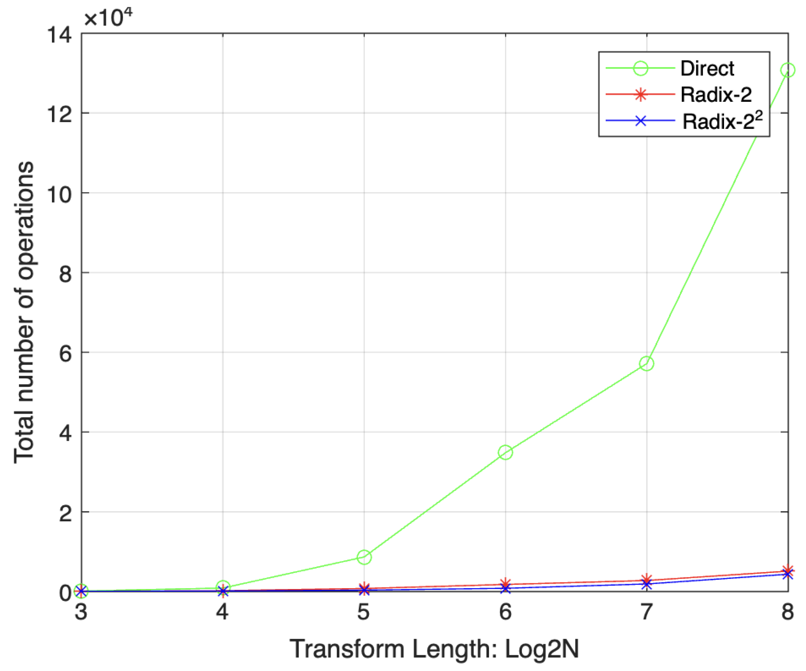
5. Arithmetic Complexity of Radix-${\mathbf{2}}^{\mathbf{2}}$ Algorithm

There are two general formulas for computing complexity: the closed formula used for single-butterfly implementation and the recursive formula used for multiple-butterfly implementation. In this paper, we used single-butterfly implementation for simplicity in calculation. The arithmetic complexity is a summation of the number of initial additions and multiplications in a single butterfly, along with the number of stages and points. A comparison of arithmetic complexity for ONMNT using direct calculations for the radix-2 and radix-$2^2$ algorithms is presented below. In the direct calculation of the transform, the numbers of addition and multiplication operations are $N(N-1)$ and $N^2$, respectively, where N is the transform length. The number of stages in the radix-2 fast algorithm is ${log}_2\left(N\right)$. Each butterfly processes $N/4$ points and requires 6 additions and 4 multiplications using the single-butterfly implementation. Therefore, the number of additions $A\left(N\right)$ and multiplications $M\left(N\right)$ for radix 2 can be calculated using the following equations:

$$\begin{array}{c}A\left(N\right)=\frac{N}{4}6{log}_2\left(N\right)=\frac{3N}{2}{log}_2\left(N\right)\end{array}$$

(67)

$$\begin{array}{c}M\left(N\right)=\frac{N}{4}4{log}_2\left(N\right)=N{log}_2\left(N\right)\end{array}$$

(68)

In the radix-$2^2$ algorithm, the number of stages S is ${log}_4\left(N\right)$ or $\frac{1}{2}{log}_2\left(N\right)$, where N is the number of points in each butterfly. The numbers of multiplication and addition operations required in each stage are 12 and 22, respectively. As the radix-$2^2$ butterfly has eight points—four main points and four retrograde points—the number of points to calculate at each stage is $\frac{N}{8}$. Therefore, the arithmetic complexity can be calculated in terms of the number of additions $A\left(N\right)$ and the number of multiplications $M\left(N\right)$ using the following equations:

$$\begin{array}{c}A\left(N\right)=\frac{N}{8}\times 22\times \frac{1}{2}{log}_{2}N=\frac{11N}{8}{log}_2\left(N\right)\end{array}$$

(69)

$$\begin{array}{c}M\left(N\right)=\frac{N}{8}\times 12\times \frac{1}{2}{log}_{2}N=\frac{3N}{4}{log}_2\left(N\right)\end{array}$$

(70)

Figure 5 shows the total calculations for direct calculations, radix-2, and radix-$2^2$, in a graph where the x-axis shows the transform length in the logarithm scale and the y-axis shows the total number of calculations, including addition and multiplication. As can be seen from the figure, both the radix-2 and radix-$2^2$ algorithms require significantly fewer calculations than the direct method. Moreover, the total number of calculations increases exponentially as the transform length increases.

Table 1. Comparison of arithmetic complexity for ONMNT using a single butterfly.

	Direct			Radix-2			Radix-22
$\mathbf{N}$	Add.	Multi.	Total	Add.	Multi.	Total	Add.	Multi.	Total
8	56	64	120	36	24	60	33	18	51
16	240	256	496	96	64	160	88	48	136
32	992	1024	2016	240	160	400	220	120	340
64	4032	4096	8128	576	384	960	528	288	816
128	16,256	16,384	32,640	1344	896	2240	1232	672	1904
256	65,280	65,536	130,816	3072	2048	5120	2816	1536	4352

presents the number of additions, multiplications, and total calculation required for ONNMT using a direct calculation as well as the radix-2 and radix-$2^2$ algorithms for transform length $N=8,16,32,64,128$ and 256. Comparing (67) and (68) with (69) and (70) for direct calculations, the numbers of saved operations in the radix-$2^2$ algorithm relative to radix 2 can be written as follows:

$$\begin{array}{c}\Delta A\left(N\right)=\frac{N}{8}{log}_2\left(N\right)\end{array}$$

(71)

$$\begin{array}{c}\Delta M\left(N\right)=\frac{N}{4}{log}_2\left(N\right)\end{array}$$

(72)

The radix-$2^2$ algorithm offers an $8.55\%$ reduction in the number of additions and a $25\%$ reduction in the number of multiplications compared to radix 2. It is important to note that the multiplication operation is more CPU-intensive than the addition operation, so a $25\%$ saving in the number of multiplications in the radix-$2^2$ algorithm is notable and makes it more suitable for a lightweight cipher application. Overall, this algorithm achieves a $15\%$ reduction in total calculations. The number of calculations for radix-4 and split radix is not included in the comparison because the transform length of radix-4 [32] fast algorithm is only limited to the power of 4, and it has more complex implementations than radix-$2^2$. Radix-$2^2$ has the same non-trivial multiplicative complexity of radix-4, but it retains the butterfly structure of radix-2 [33]. The saving percentage will be higher as the transform length increases.

6. An Example of the Proposed Fast Algorithm

To validate the accuracy of the derived algorithm, a short data packet was transformed using the radix-$2^2$ fast algorithm for the ONMNT forward transform. Then, IONMNT was applied to the transformed data using the radix-$2^2$ algorithm to recover the original data. The experiment was implemented in the C programming language. Moreover, the outputs of the proposed fast algorithm for forward ONMNT and IONMNT were compared with the direct calculations and verified. A brief description of the experiment and the results are presented below:

6.1. Forward ONMNT Transform

First, the text “Encryption story” was converted into ASCII values and transformed using the proposed algorithm with transform parameters ${\alpha }_1=2$, ${\alpha }_2=3$, $N=16$, $p=7$, $M_p=127$, $n=\{0,1,2,\cdots ,15\}$, and $k=\{0,1,2,\cdots ,15\}$. The original and transformed values are as follows:

x[n]:	69	110	99	114	121	112	116	105	111	110	32	115	116	111	114	121
X[k]:	56	52	33	52	53	35	83	80	85	82	14	63	21	113	79	76

6.2. IONMNT Transform

IONMNT was applied to the transformed data $X\left[k\right]$ using the same transform parameters, recovering the original data. Moreover, the results match with the direct calculations.

X[k]:	56	52	43	52	53	35	83	80	85	82	14	63	21	113	79	76
x[n]:	69	110	99	114	121	112	116	105	111	110	32	115	116	111	114	121

Therefore, this experiment confirms the proposed solution’s validity and shows no rounding or truncation errors, which is a good attribute of the ONMNT.

7. Conclusions

An efficient derivation of a radix-$2^2$ fast algorithm for both ONMNT and IONMNT has been presented in this paper. A bit-unscrambling technique provides a more straightforward implementation of the radix-$2^2$ algorithm compared to traditional multidimensional index mapping. The butterfly and signal flow diagrams presented in the paper offer flexibility in implementing ONMNT using the radix $2^2$ algorithm. The proposed fast algorithm offers an $8.55\%$ reduction in the number of additions, a $25\%$ reduction in the CPU-intensive multiplication operations, and an overall reduction of $15\%$ compared to radix-2 while retaining the butterfly structure of radix-2. This efficient and fast algorithm can be used for lightweight ciphers and hash functions to take advantage of both the reduced number of calculations offered by the radix-4 algorithm and the simple butterfly structure of the radix-2 fast algorithm. In future research, the proposed algorithm could be implemented in multiple hardware platforms and used in real-life applications to understand its performance better. Moreover, the derivation could also be extended to O²NMNT.

References

- Nussbaumer, H.J. Number Theoretic Transforms, 2nd ed.; Springer: Berlin/Heidelberg, Germany, 1982; pp. 211–240. [Google Scholar] [CrossRef]
- Yan, K. A Review of the Development and Applications of Number Theory. J. Phys. Conf. Ser. 2019, 1325, 012128. [Google Scholar] [CrossRef]
- Rader, C.M. Discrete convolutions via Mersenne transforms. IEEE Trans. Comput. 1972, C-21, 1269–1273. [Google Scholar] [CrossRef]
- Kehil, D.; Ferdi, Y. Signal encryption using new Mersenne number transform. In Proceedings of the 2010 7th International Symposium on Communication Systems, Networks Digital Signal Processing (CSNDSP 2010), Newcastle Upon Tyne, UK, 21–23 July 2010; pp. 736–740. [Google Scholar] [CrossRef]
- Křížek, M.; Luca, F.; Somer, L. Fermat number transform and other applications. In 17 Lectures on Fermat Numbers: From Number Theory to Geometry; Springer: New York, NY, USA, 2001; pp. 165–186. [Google Scholar] [CrossRef]
- Agarwal, R.C.; Burrus, C.S. Fast convolution using Fermat number transforms with applications to digital filtering. IEEE Trans. Acoust. 1974, 22, 87–97. [Google Scholar] [CrossRef]
- Boussakta, S.; Holt, A.G.J. New number theoretic transform. Electron. Lett. 1992, 28, 1683–1684. [Google Scholar] [CrossRef]
- Boussakta, S.; Hamood, M.T.; Rutter, N. Generalized new Mersenne number transforms. IEEE Trans. Signal Process. 2012, 60, 2640–2647. [Google Scholar] [CrossRef]
- Rutter, N. Implementation and Analysis of the Generalised New Mersenne Number Transforms for Encryption. Ph.D. Thesis, Newcastle University, Newcastle upon Tyne, UK, 2015. Available online: http://theses.ncl.ac.uk/jspui/handle/10443/3236 (accessed on 25 July 2023).
- Hamood, M.T. Development of Efficient Algorithms for Fast Compution of Discrete Transforms. Ph.D. Thesis, Newcastle University, Newcastle upon Tyne, UK, 2012. [Google Scholar]
- Hua, J.; Liu, F.; Xu, Z.; Li, F.; Wang, D. A fast realization of new Mersenne number transformation and its applications. Int. J. Circuit Theory Appl. 2019, 47, 738–752. [Google Scholar] [CrossRef]
- He, S.; Torkelson, M. New approach to pipeline FFT processor. In Proceedings of the International Conference on Parallel Processing, Honolulu, HI, USA, 15–19 April 1996; pp. 766–770. [Google Scholar] [CrossRef]
- Pollard, J.M. The Fast Fourier Transform in a Finite Field. Math. Compulation 1971, 25, 365–374. [Google Scholar] [CrossRef]
- Cortés, A.; Vélez, I.; Sevillano, J.F. Radix rk FFTs: Matricial representation and SDC/SDF pipeline implementation. IEEE Trans. Signal Process. 2009, 57, 2824–2839. [Google Scholar] [CrossRef]
- Anguraj, P.; Krishnan, T.; Natesan, K. Design of an area-efficient various N-point support radix-2/22 FFT using modified butterfly units. Int. J. Recent Tech. Eng. 2019, 8, 10189–10198. [Google Scholar] [CrossRef]
- Samir Algnabi, Y.; Teymourzadeh, R.; Othman, M.; Shabiul Islam, M. FPGA implementation of pipeline digit-slicing multiplier-less radix 22 DIF SDF butterfly for fast Fourier transform structure. arXiv 2018, arXiv:1806.04570. [Google Scholar]
- Santhosh, L.; Thomas, A. Implementation of radix 2 and radix 22 FFT algorithms on Spartan6 FPGA. In Proceedings of the 2013 Fourth International Conference on Computing, Communications and Networking Technologies (ICCCNT), Tiruchengode, India, 4–6 July 2013; pp. 1–4. [Google Scholar] [CrossRef]
- Li, N.; Van Der Meijs, N.P. A radix 22 based parallel pipeline FFT processor for MB-OFDM UWB system. In Proceedings of the 2009 IEEE International SOC Conference (SOCC), Belfast, UK, 9–11 September 2009; pp. 383–385. [Google Scholar] [CrossRef]
- Eisenbarth, T.; Kumar, S.; Paar, C.; Poschmann, A.; Uhsadel, L. A Survey of Lightweight-Cryptography Implementations. IEEE Des. Test Comput. 2007, 24, 522–533. [Google Scholar] [CrossRef]
- Philip, M.A.; Vaithiyanathan. A survey on lightweight ciphers for IoT devices. In Proceedings of the 2017 International Conference on Technological Advancements in Power and Energy (TAP Energy), Kollam, India, 21–23 December 2017; pp. 1–4. [Google Scholar] [CrossRef]
- Fragkos, G.; Minwalla, C.; Plusquellic, J.; Tsiropoulou, E.E. Artificially Intelligent Electronic Money. IEEE Consum. Electron. Mag. 2021, 10, 81–89. [Google Scholar] [CrossRef]
- Parvatham, N.; Professor, A. LEA-SIoT: Hardware Architecture of Lightweight Encryption Algorithm for Secure IoT on FPGA Platform. (IJACSA) Int. J. Adv. Comput. Sci. Appl. 2020, 11, 720–725. [Google Scholar] [CrossRef]
- Nabeel, N.; Habaebi, M.H.; Rafiqul Islam, M. LNMNT—New Mersenne number based lightweight crypto hash function for IoT. In Proceedings of the 8th International Conference on Computer and Communication Engineering, ICCCE 2021, Kuala Lumpur, Malaysia, 22–23 June 2021; pp. 68–71. [Google Scholar] [CrossRef]
- Maetouq, A.; Daud, S.M. HMNT: Hash function based on new Mersenne number transform. IEEE Access 2020, 8, 80395–80407. [Google Scholar] [CrossRef]
- Nabeel, N.; Habaebi, M.H.; Islam, M.D.R. Security analysis of LNMNT-lightweight crypto hash function for IoT. IEEE Access 2021, 9, 165754–165765. [Google Scholar] [CrossRef]
- Burrus, C. Index mappings for multidimensional formulation of the DFT and convolution. IEEE Trans. Acoust. Speech Signal Process. 1977, 25, 239–242. [Google Scholar] [CrossRef]
- Burrus, C. Bit reverse unscrambling for a radix-2M FFT. In Proceedings of the ICASSP ’87, IEEE International Conference on Acoustics, Speech, and Signal Processing, Dallas, TX, USA, 6–9 April 1987; Volume 12, pp. 1809–1810. [Google Scholar] [CrossRef]
- Burrus, C.S. Unscrambling for fast DFT algorithms. IEEE Trans. Acoust. Speech Signal Process. 1988, 36, 1086–1087. [Google Scholar] [CrossRef]
- Papamichalis, P.E.; Burrus, C.S. Conversion of digit-reversed to bit-reversed order in FFT algorithms. In Proceedings of the International Conference on Acoustics, Speech, and Signal Processing, Glasgow, UK, 23–26 May 1989; Volume 2, pp. 984–987. [Google Scholar] [CrossRef]
- Hamood, M.T.; Boussakta, S. Efficient algorithms for computing the new Mersenne number transform. Digit. Signal Process. 2014, 25, 280–288. [Google Scholar] [CrossRef]
- Agarwal, R.C.; Burrus, C.S. Number theoretic transforms to implement fast digital convolution. Proc. IEEE Inst. Electr. Electron. Eng. 1975, 63, 550–560. [Google Scholar] [CrossRef]
- Chu, E.; George, A. Inside the FFT Black Box—Serial and Parallel Fast the Serial and Parallel Fast Algorithms; CRC Press: Boca Raton, FL, USA, 2000; pp. 109–117. [Google Scholar]
- Selvakumar, S.; Stephy Jasmine Rani, L.; Vijayalakshmi, G.; Vishnudevi, N.; Janakiraman, N. Radix 25 Fft Architecture Implementation In Xilinx Fpga. In Proceedings of the 2014 International Conference on Innovations in Engineering and Technology, Tamil Nadu, India, 21–22 March 2014; pp. 1507–1511. [Google Scholar]