1. Introduction
Humans can identify patterns and objects, such as a clock, a chair, a dog, or a cat. However, for a computational model, pattern analysis is a considerable challenge. Using artificial intelligence (AI) [
1] makes it possible for computer systems to perform pattern recognition. However, it is necessary to develop models capable of learning. Through these models, it is possible to achieve methods that align with how the human brain performs the analysis. Machine learning (ML) [
2] can be seen as a subtopic of AI, whose algorithms make it possible for software applications to have high accuracy in predicting outcomes, even if they have not been specifically programmed to do so.
ML is translated into the execution of algorithms, thus automatically creating models capable of learning based on a set of data. It is necessary to train the ML models, giving them an appropriate set of data so that in this training process, the employed algorithm “learns”, and iteratively adjusts itself. After training, the created model can make predictions with a high assertiveness value. Despite the substantial number of algorithms developed for ML, artificial neural networks (ANNs) have consistently been demonstrated to be the most adaptable, especially with the emergence of deep learning (DL) [
3]. Theoretically, one can use ANNs for the detection of complex patterns, such as those present in images, but in practice, it may be unfeasible due to the number of calculations required being extremely high. This occurs because in a conventional ANN, each pixel is connected to each neuron. In this case, the computational load added makes the network unfeasible for image analysis [
4].
Convolutional neural networks (CNNs) have made pattern recognition in images feasible. When considering an image, the proximity of the pixels has a strong correlation, and the CNNs specifically use this relationship. Nearby pixels have a higher probability of being related than pixels further apart. Convolution solves the problem of the need for a high number of connections that occurs in conventional ANNs, making it possible to process images by filtering connections by proximity. In a given layer, instead of connecting each input to each neuron, CNNs restrict the connections intentionally so that any neuron accepts inputs only from a small part of the previous layer (such as 5 × 5 or 3 × 3 pixels).
The evolution of graphics processing units (GPUs) and the availability of libraries, such as TensorFlow (TF) [
5] and Keras [
6], have substantially facilitated the development of CNNs. Despite the high accuracy that DL-based models can achieve, the problem associated with the level of confidence that the user has in the prediction of the network still remains. This can be solved through the use of probabilistic models (PMs), as they allow the expression of epistemic uncertainty in the predictions generated by the models. These models are computationally demanding and have only recently become feasible with the development of variational inference (VI) [
7]. The creation of probabilistic CNNs became simpler through the emergence of models based on the estimators, such as Flipout, and their inclusion in TF probability [
8].
Pre-trained deterministic models (DMs) with conventional architectures are available with optimization performed on large data sets, allowing transfer techniques to be used to achieve high accuracy. However, PMs do not yet have this transfer option because, typically, the distributions that these models learn are strongly associated with the data used to train the models. Thus, it is usually necessary to fully train the models on the train data sets, whose distributions should be learned.
One of the biggest barriers to the use of DL models by inexperienced users is the complexity associated with programming the components. Actually, the need for tools that can help the development of ML models has been identified since the beginning of this field. However, more recently, the Classification Lerner Application from Matlab [
9] employed an innovative approach to address this need. It uses a simple button-based interface with short messages to guide the user, allowing any user to develop conventional ML models without requiring a deep understanding of all concepts underlying the models, having only to know how to use the developed model. This no-code approach allows for accelerating the use of these models in diverse areas of knowledge. With the large interest that ML has attracted in recent years, some newer platforms aimed at addressing this need for simple-to-use platforms for ML development. An example of such a platform is the Orange Data Mining application [
10], which is free and developed in Python. It is also based on a simple button-based interface with small messages to guide the user.
By analyzing the state-of-the-art of GUIs for developing ML models, a gap was found concerning the PMs, especially with probabilistic CNNs. This gap is of particular relevance since these models require high knowledge in the areas of statistics and DL. Additionally, there is still little documentation on the procedures necessary for the development of these models. This restricts the mass use of these models, being only accessible to specialists with knowledge in the area. Considering the great interest that DL based on probabilistic CNNs has had recently, especially by programmers interested in making applications for pattern recognition, it becomes necessary to obtain a simple, user-friendly, and easy-to-use alternative that allows the creation of the models.
Therefore, the main objective of this work was the development of a graphical user interface (GUI) that allows any user without previous knowledge in the area of DL, giving the capability to develop PMs based on CNNs with a no-code approach that follows Matlab’s Classification Learner Application concept. Two processes were developed; one containing models with standard architectures in the DL area, and another where the user can create a model layer by layer with the desired architecture, with the possibility of selecting the desired number and type of layers and their characteristics.
This work has the following organization: presentation of the materials and methods in
Section 2; performance assessment of the developed algorithms in
Section 3; discussion of the results in
Section 4; and conclusions of the work in
Section 5.
2. Materials and Methods
The developed GUI presents multiple options that guide the user in the process of selecting the architecture of the ANN to be developed, defining the training procedure, and obtaining the resulting model in a simple and intuitive manner. However, it also allows the inexperienced user to train models with a small number of choices using the pre-defined recommended values for the options. It is only necessary to load the data sets, select the desired model, and start training it. Essentially, the developed GUI was designed to allow the development of a probabilistic CNN to be done in three steps: insertion of the desired parameters for training and choice of the architecture; training of the model; and visualization of the results.
When developing CNNs, one of the first issues that occur is choosing the architecture to be used. This defines the types and sequence of layers, the parameters, the number of inputs, the number of outputs, and the activation functions (AFs). All these options are available in the developed GUI, and the user can either choose the recommended (default) options or can select the available alternatives. If needed, the user can develop new modules for the GUI or edit the existing ones.
The entire code was developed in Python 3, including the GUI and the development of the models, and is available (in open source) in the public repository: (
https://github.com/achaves37/Interface-Grafica-para-desenvolvimento-de-Redes-Neuronais-Convolucionais-Probabiliticas/, accessed on 2 February 2023). Two versions are provided, one called “TestInterface” and another called “Interface”. In the latter, the user will need to load his data sets, which are intended to be used for developing the custom models. In contrast, the first uses standard ML datasets (useful for testing proposed architectures and getting familiarized with the interface). All the code is documented and organized to make it possible to add/edit some models in a simple and direct way. It is recommended that users be familiar with basic operations with a Python console [
11]. The user and the program interact through Tkinter [
12] and IPython. The PMs were also developed in Python, using the TF libraries. However, the computational performance is not affected by the choice of this language because TF internally converts the models described for the compute unified device architecture (CUDA) [
13], C++, and is optimized for GPU use.
2.1. Convolutional Neural Networks
CNNs are usually developed to be deterministic and are associated with pattern recognition in images or signals, presenting a high efficiency in classification. The process of data classification by the networks is carried out by means of the several layers that compose them [
14]. These layers are typically of three types: convolution, pooling, and dense. A data alteration by ANNs takes place in all these layers, usually having non-linear AFs, such as the rectified linear unit (ReLU), to increase the learning capacity. The input and output layers are the ones that interact with the outside (they are not hidden).
CNNs use filters that consist of randomly initialized weights, subsequently updated at each new input, through the back-propagation algorithm to learn the patterns. The region of the input, where the filter is applied, is called the receptive field. Pooling is used to reduce the information from the previous layer, decreasing the number of weights to be learned and avoiding overfitting [
15]. As in convolution, an area unit is chosen to traverse the entire output of the previous layer. Furthermore, it is necessary to choose how the filtering will be done. The most used is the choice of the maximum value (maxpooling), where only the largest number of the unit is passed to the output.
2.2. Probabilistic Models
One of the main advantages of PMs over DMs is the ability to present the epistemic uncertainty of predictions. However, the development of these PMs is typically more complex, requiring additional knowledge on how to build them, frequently using VI approximation [
16]. It allows approximating probabilistic inference as an optimization problem, searching for an alternative a posteriori distribution that minimizes the Kullback–Leibler divergence (KLD) [
17] with the true a posteriori distribution. In this way, all the weights
W of the network are replaced by a probabilistic distribution, and the distribution is optimized during network training. In this case, the Gaussian distribution [
18] is often used to represent these distributions.
Specifically, VI involves selecting a member
q from a family of distributions
Q, which is similar to the target distribution using KLD to measure the fit. In essence, the idea behind variational inference is to reframe our approximate Bayesian inference problem as an optimization problem. This reframing enables the leverage of the full range of mathematical optimization techniques to tackle the problem. By optimizing the parameters, denoted as
, for
q, the solution that is closest to the conditional interest P(
W|
D) can be found using KLD, where
D is the training data. The optimal solution can be obtained by solving [
16]
Since P(
W|
D) is unknown, a different objective needs to be optimized in order to minimize the KLD. The standard approach is to use the evidence lower bound (ELBO), which can be calculated by [
16]
The cost function can be seen as a composition of two parts. The first part of the function is typically viewed as the complexity cost, which leads to the search for solutions whose densities are close to the prior. The second part is dependent on the data; it is usually referred to as the likelihood cost because it describes the probability of the data given to the model, leading to solutions that better explain the observed data. As a result, this cost function interprets a compromise between satisfying the simplicity of the prior probability distribution P(W) and the complexity of the data.
Although this approximation can be achieved through VI, using a prior distribution of the model weights to produce a regularization effect, the exact calculation of the ELBO as presented is computationally prohibitive. Another relevant aspect is the usual approach of using a Gaussian distribution for the model weights, with two parameters, the mean and the standard deviation, as it facilitates implementation. An approximation of the ELBO is required to enable the optimization of the network with gradient descent methods based on this loss function. This approximation is given by [
16]
To decrease the time required to train the networks, the Flipout estimator [
19] is used to minimize the ELBO. Therefore, the output of each layer for all examples in the subgroup
X, considering the activation function
and the average weights
, is given by [
19]
Since
A and
B are independently sampled from
and
, it is possible to backpropagate with respect to
X,
, and
, optimizing, in this way, the network parameters. In short, VI directly approximates the posterior distribution with a simpler distribution, avoiding the calculation of the likelihood of all occurrences [
20].
2.3. Graphical Interface
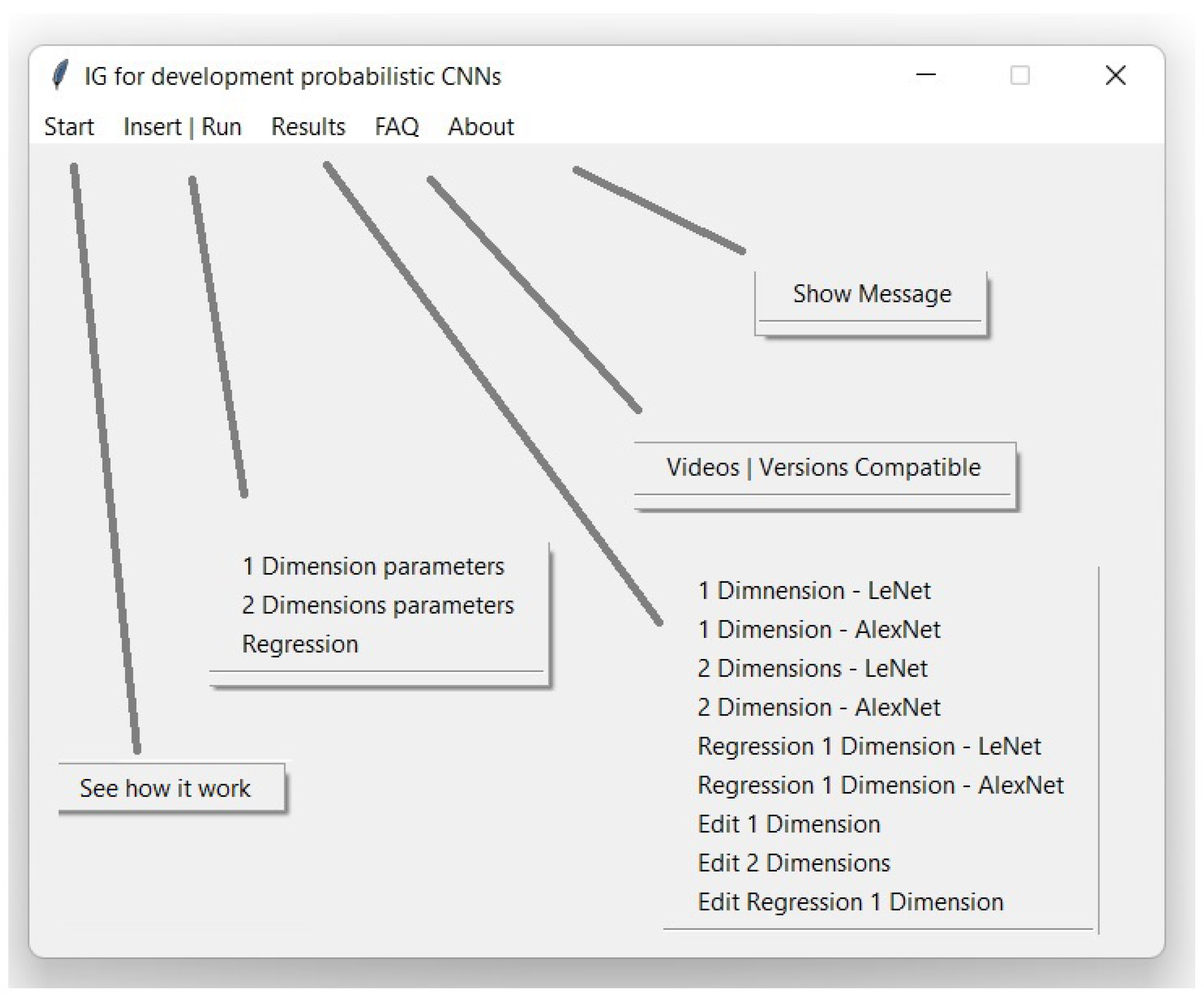
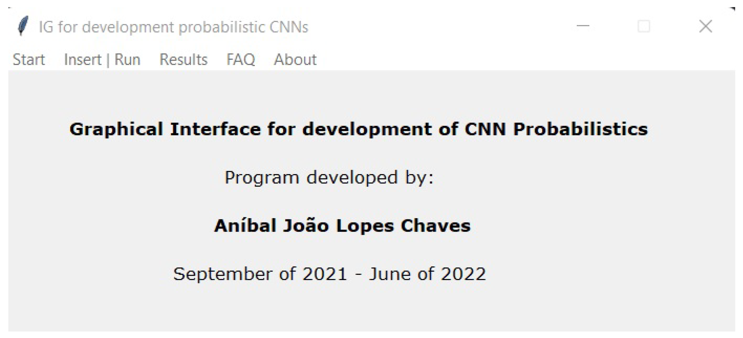
The developed GUI is shown in
Figure 1. This is made up of five tabs:
The first tab, called “Start” gives a brief summary of how the application works in order to use the different data sets.
On the second tab, denoted as “Insert|Run”, the user can edit the parameters to develop the desired model and then train the model.
The third tab, named “Results”, allows the user to visualize the results.
Lastly, the fifth tab, called “About”, displays a message about the authorship of the development of the GUI.
In
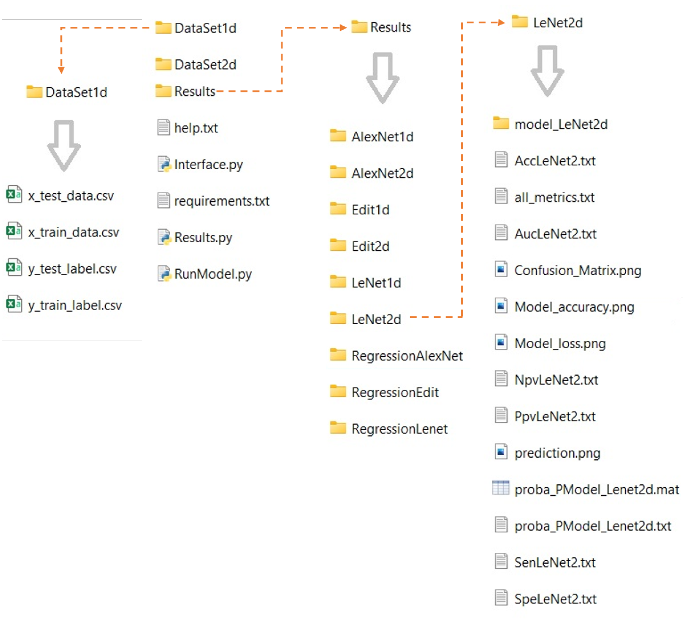
Figure 2, the “Start” tab is presented, where GUI provides information regarding its use for all datasets. The GUI obtains data from four comma-separated value (CSV) files (stored in specific folders such as DataSet1d or DataSet2d for one- or two-dimensional classification data, respectively), using one for training data, one for training labels, one for testing data, and one for testing labels. The data for training and testing must be organized in rows, where each row represents a sample, and each column denotes a feature of the sample. If two-dimensional data are being used, they must be flattened, and the program will internally recreate the original shape to feed the models. Additionally, the labels file should have one row for each sample in the data file (matching the raw number in the files) and be encoded in decimal or one hot encoding. The user can carry out preprocessing of the data, such as normalization or standardization, and the result can be stored in the data CSV files. All generated results will also be stored in folders according to the used model, as shown in
Figure 3.
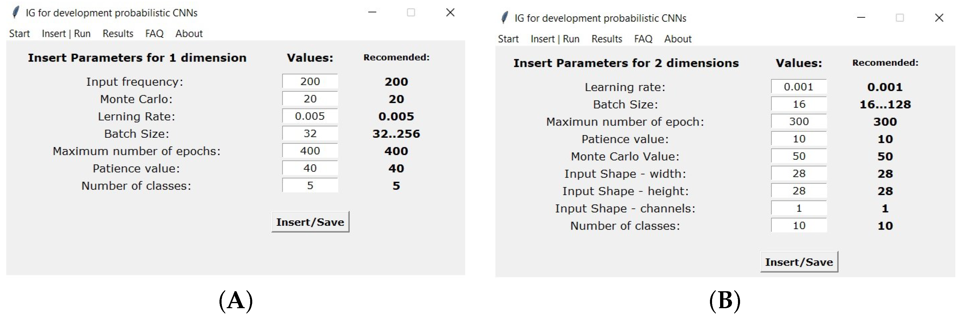
The subsequent tab called “Insert|Run” is shown in
Figure 4. Here, the user can introduce the parameters that will control the models’ training. If necessary, the user can compare with the recommended values. These values are already pre-filled, and if the user wants to use those values, he only has to click on the “Insert|Save” button. Otherwise, the user must insert the values and then press the button. By pressing the button, the confirmation message is shown on the IPython console (for visual confirmation of the parameters previously inserted), as shown in the example of
Figure 5. The left side of the
Figure 5 is for classification using a one-dimensional data set, and the right side is for a regression two-dimensional data set using. The user can also perform regression with one-dimensional data and classification with two-dimensional data. If needed to expand to higher dimensions, the user can add new modules (or edit an existing one) to the GUI, copying the code from the two-dimensional models and changing the number of dimensions to the desired value.
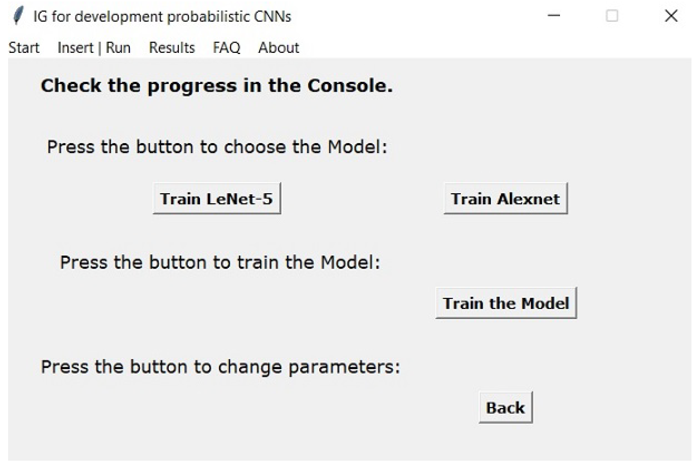
Figure 6 shows the tab named “Insert|Run”. Here, the user can select which standard model should be trained, or, if preferred, create a model (create layer by layer). If needed, the user can add new standard architectures (or edit the existing ones) to the GUI, requiring only adding the structure of the model to a predefined file. The default optimizer is the ADAM algorithm. However, the user can change to another optimizer if needed. Additionally, accuracy was the tracked metric for classification while the mean squared error was the examined metric for regression. The training process is already prepared to perform early stopping if a minimum improvement is not attained in a sequence of epochs defined by the user (if the user does not pretend to use early stopping, then it just needs to specify the patience value to be higher than the number of epochs intended to be executed).
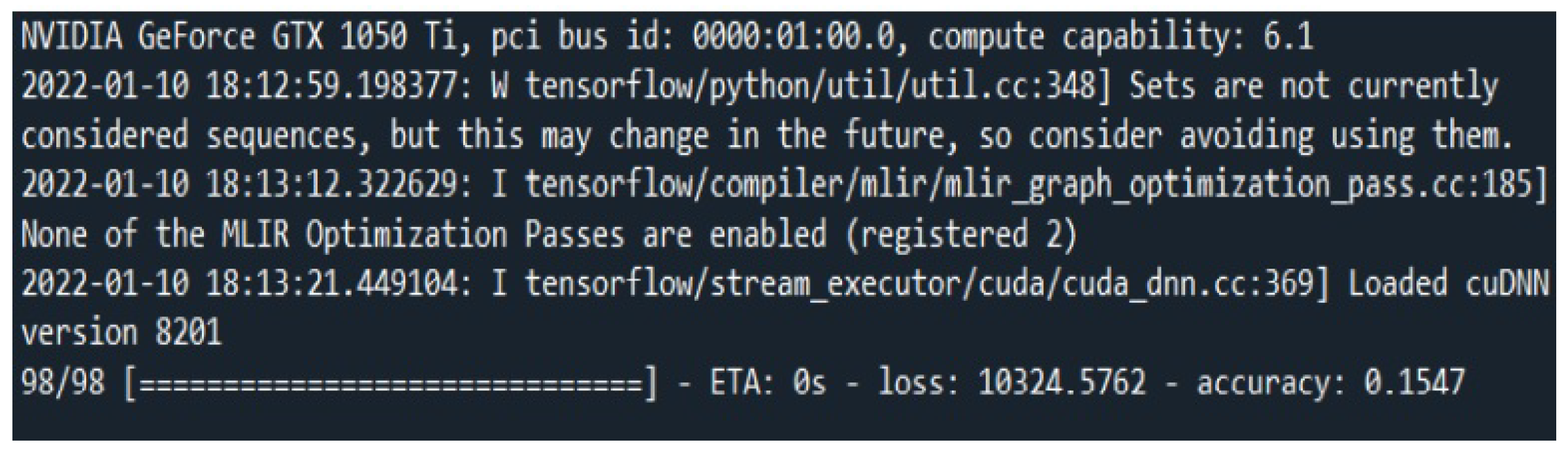
After pressing the “Train Model” button, the program starts training the selected model.
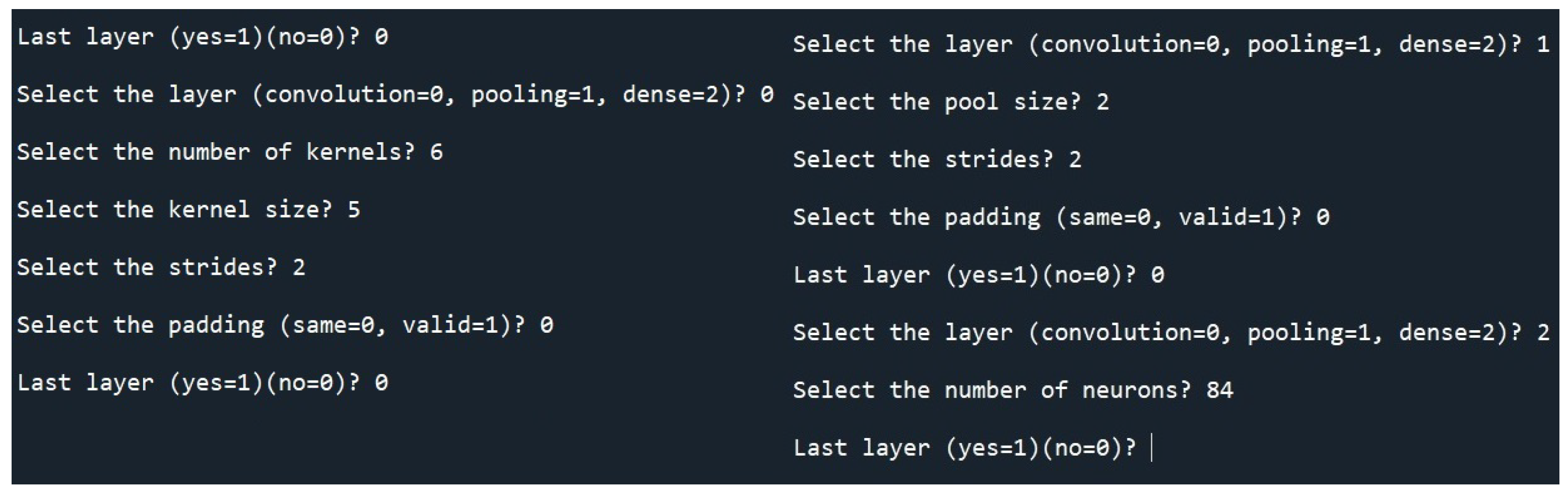
Figure 7 shows the console indicating the progress in training the model. Furthermore, the user can create the model by inserting it layer by layer, having to select the layer type; in this case, convolution, pooling, or dense. The insertion window is shown in
Figure 8.
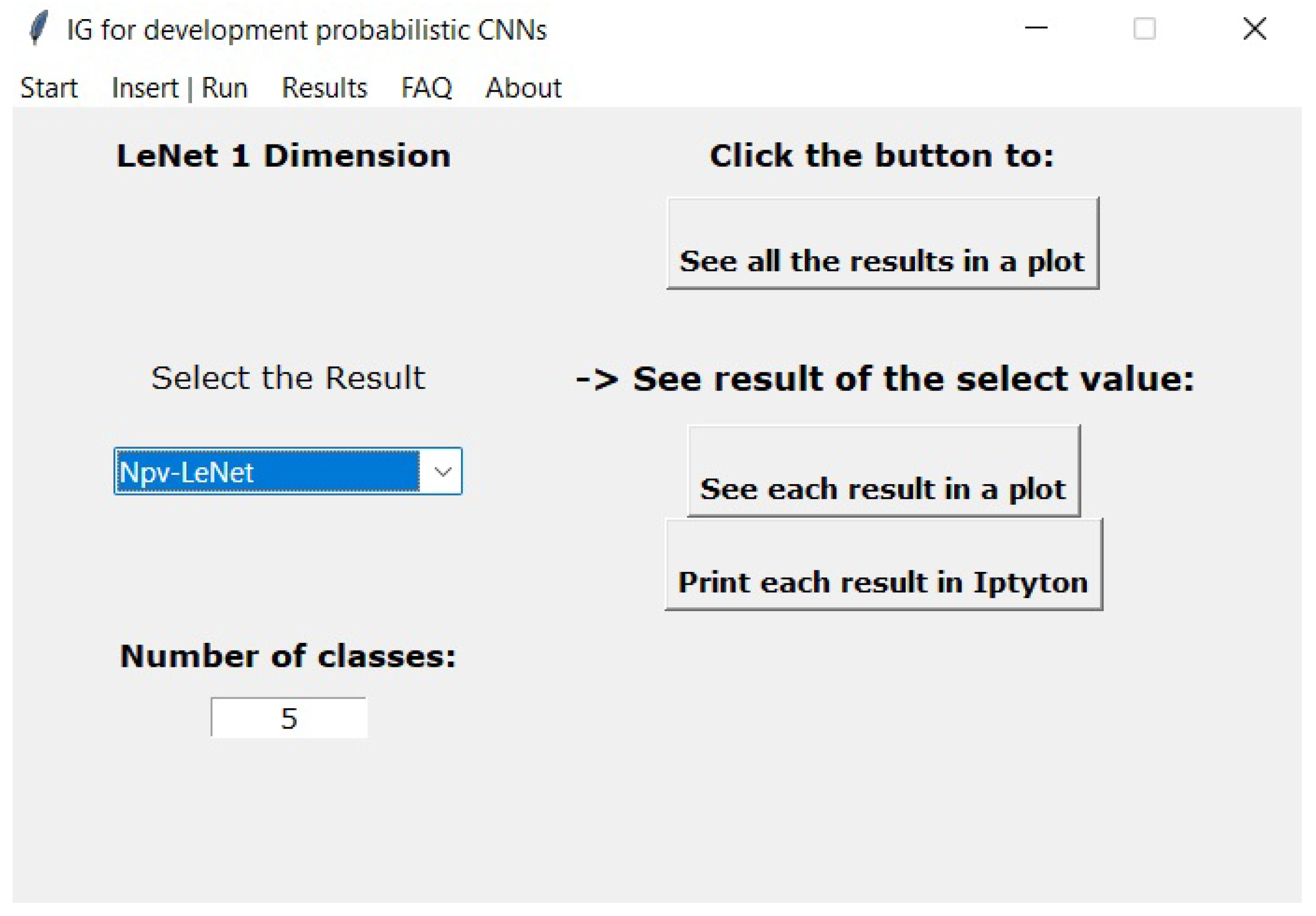
In the “Results” menu, shown in
Figure 9, the results of the models’ training are presented. The user is required to select which model should be examined. Pressing “See all the results in a plot” displays a single plot with all performance metrics. Furthermore, pressing “See each result in a plot” displays one plot with the chosen performance metric to be plotted. Pressing “Print each result in IPython” displays the values in the IPython console.
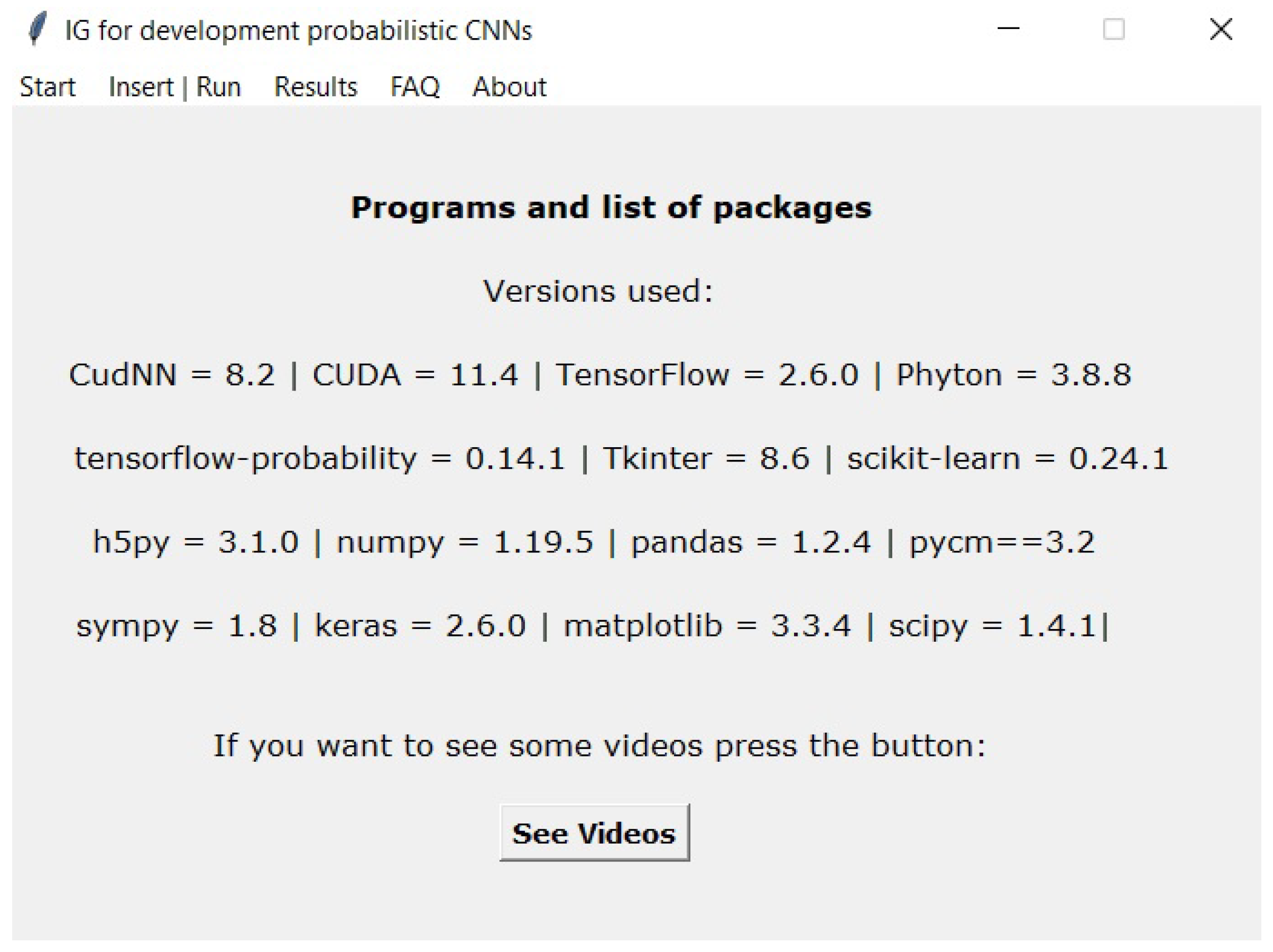
The tab denoted “FAQ”, represented in
Figure 10, shows the user information about libraries that should be installed and checks if they are present in the system. Lastly, the “About” tab, represented by
Figure 11, shows the user information about GUI development.
3. Interface Development
The developed GUI was developed in three iterations by having first meetings with machine learning specialists to highlight which requisites they consider to be essential for the tool. A quality attribute workshop was then carried out by five specialists to vote on which requisites they consider relevant. The identified requisites, their attribute, and the number of votes were as follows:
The GUI should allow the examination of 1D and 2D data while keeping the option to easily integrate higher-dimensional data. Usability attribute voted as relevant by three specialists.
The GUI should have standard default parameters to help the inexperienced user. Usability attribute voted as relevant by three specialists.
The GUI should allow the default parameters to be changed and to easily add new elements to its code. Usability attribute voted as relevant by three specialists.
The GUI should allow the user to develop PM based on CNN for both regression and classification problems. Usability attribute voted as relevant by five specialists.
The GUI should allow the user to change the model’s architecture. Usability attribute voted as relevant by two specialists.
The GUI should be responsive to the user commands, while requiring no coding from the user side to develop a model. Usability attribute voted as relevant by four specialists.
The GUI should provide the user with feedback when an error occurs, specifying the source of the error. Testability attribute voted as relevant by two specialists.
It should be possible to transition between any tab in less than 5 s. Performance attribute voted as relevant by four specialists.
When the training procedure finishes, the model and the performance results (training and testing) should be saved and made available for the user. Availability attribute voted as relevant by three specialists.
The GUI execution should be independent of the operating system. Interoperability attribute voted as relevant by two specialists.
The GUI should provide feedback to the user during the training procedure. Availability attribute voted as relevant by two specialists.
The GUI should provide the user with a list of all parameters that are going to be used to train the model. Usability attribute voted as relevant by two specialists.
From the carried-out workshop, it was concluded that the main concerns focused on usability issues related to the graphical interface, i.e., how easy it is for the user to perform tasks. Therefore, the graphical user interface was developed to benefit the usability quality attribute the most.
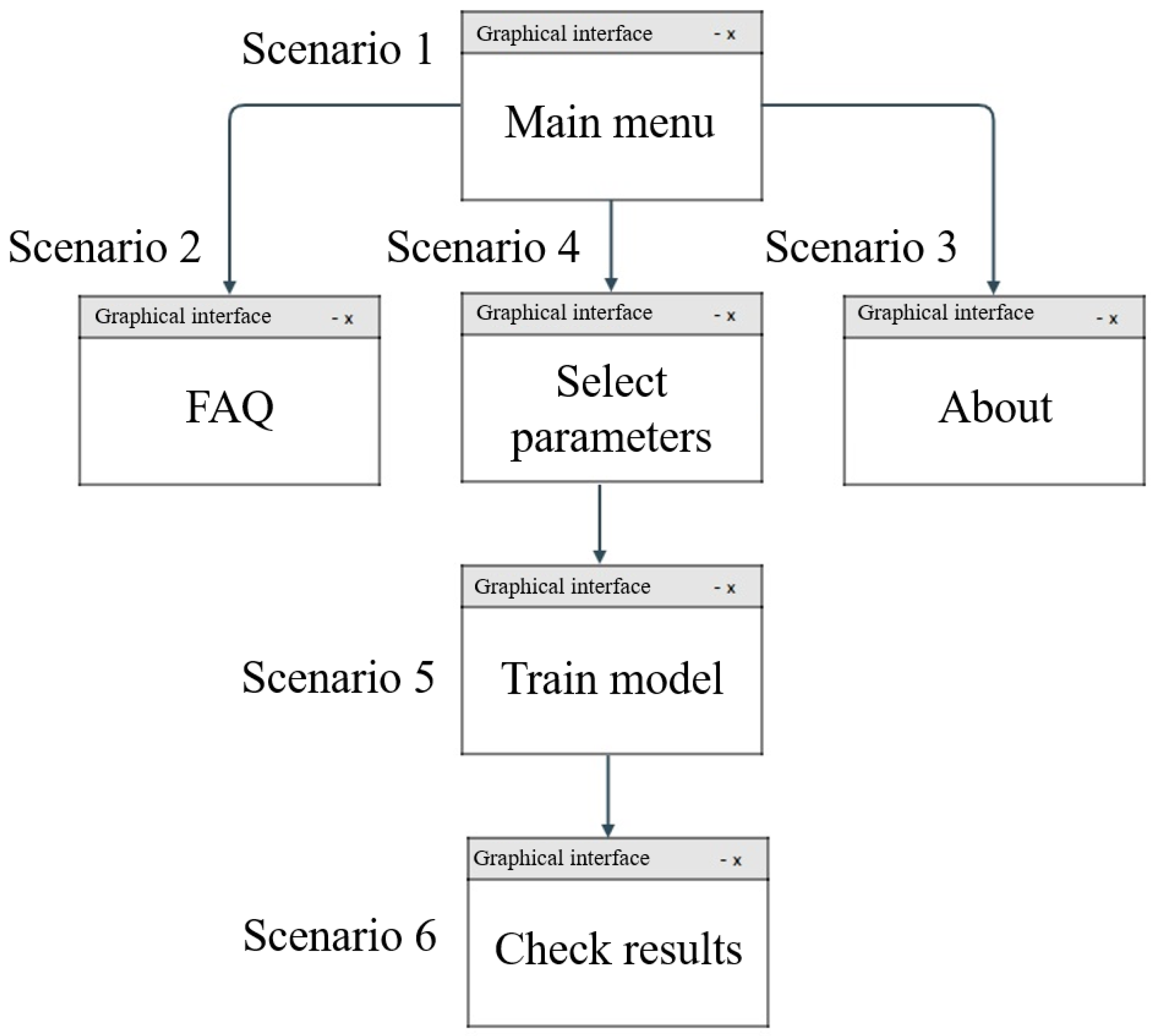
The second iteration was a discussion with GUI specialists on how to properly present all functionalities while using a simple functionality-oriented interface. After defining the desired entity-relationship model and the use case diagram, a navigation map was proposed with six main scenarios as depicted in
Figure 12. These scenarios were as follows:
Scenario 1: represents the beginning of the GUI; information is displayed to guide the user in the process of using the GUI.
Scenario 2: presents the most frequent questions regarding the use of the GUI.
Scenario 3: contains the GUI development information.
Scenario 4: in this scenario, the parameters for the model must be inserted; the parameters differ for different datasets, being possible to choose the model with predefined architecture or create a model with the architecture defined layer by layer.
Scenario 5: after choosing or editing the model, it is possible to proceed to the training procedure, developing the desired model.
Scenario 6: in this scenario, it is possible to observe the results in different ways.
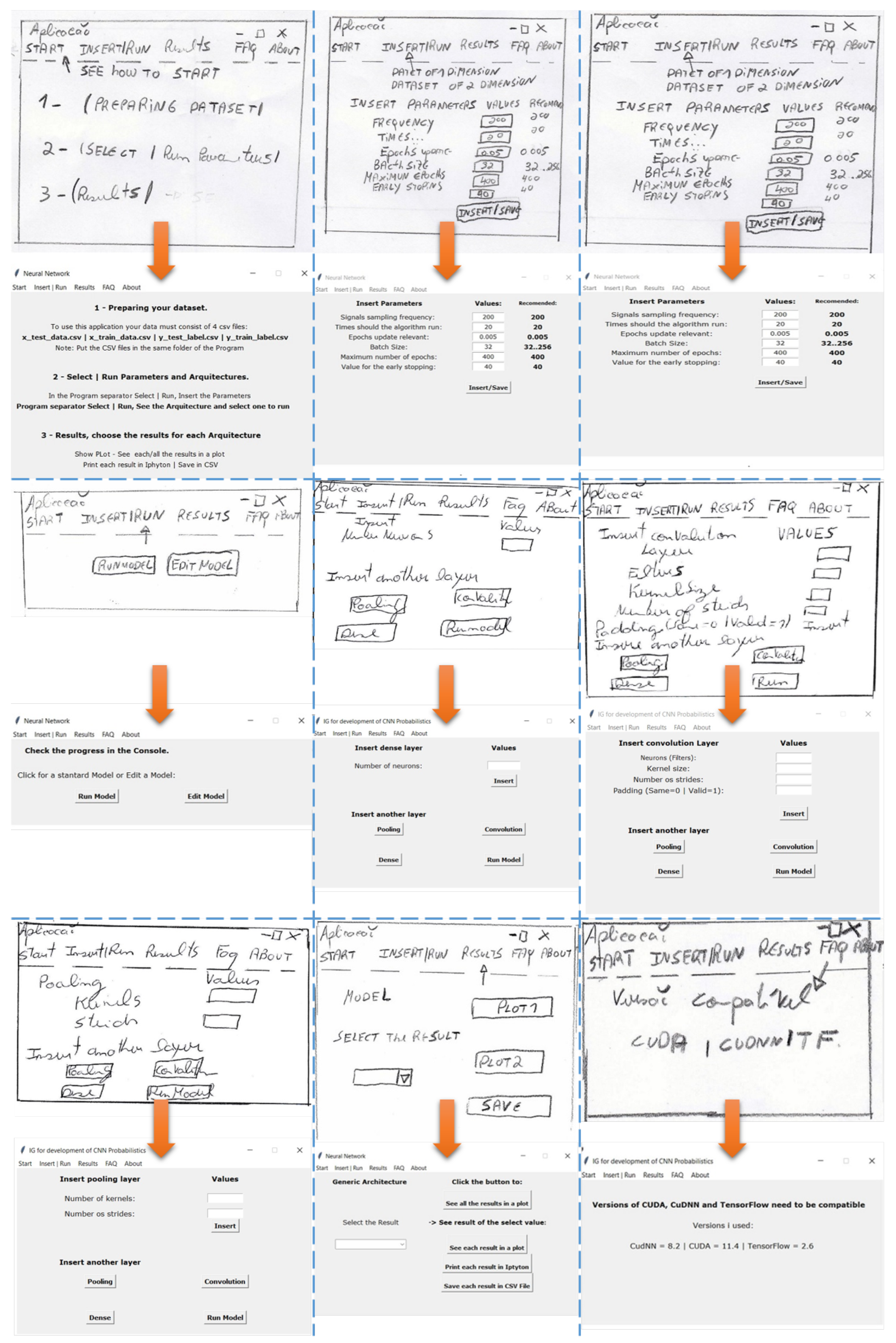
Low- and high-fidelity prototypes were made with the specialist during this second iteration.
Figure 13 shows all created prototypes, depicting low-fidelity on the top and high-fidelity on the bottom. Usability tests were carried out in the last iteration, which was performed on 13 subjects (ten males and two females) with an age range of 25 to 36 years old (average of 29.4). All subjects had used machine learning before, with eight subjects reporting having substantial experience, while the remaining five reported having minimal to some experience.
Several tasks were created to cover all potential usage scenarios, each requiring the selection of a model, training, and analysis of results. Once the tasks were completed, the system usability scale [
21] was utilized to assess the system’s performance. The outcomes showed an average score of 4.4 out of 5, equivalent to 88%, which falls under the “Excellent” category.
During the test, the users identified two main flaws in the high-fidelity prototypes. The first one was the lack of a button to go back if, by mistake, they chose the wrong model (it required the user to restart the GUI to do so); hence, a button to add this functionality was included. The second one was the lack of relevant information presented in the “FAQ” tab. This problem was addressed by adding a button that leads the user to video tutorials and by including more information regarding the versions of the sued libraries.
4. Results
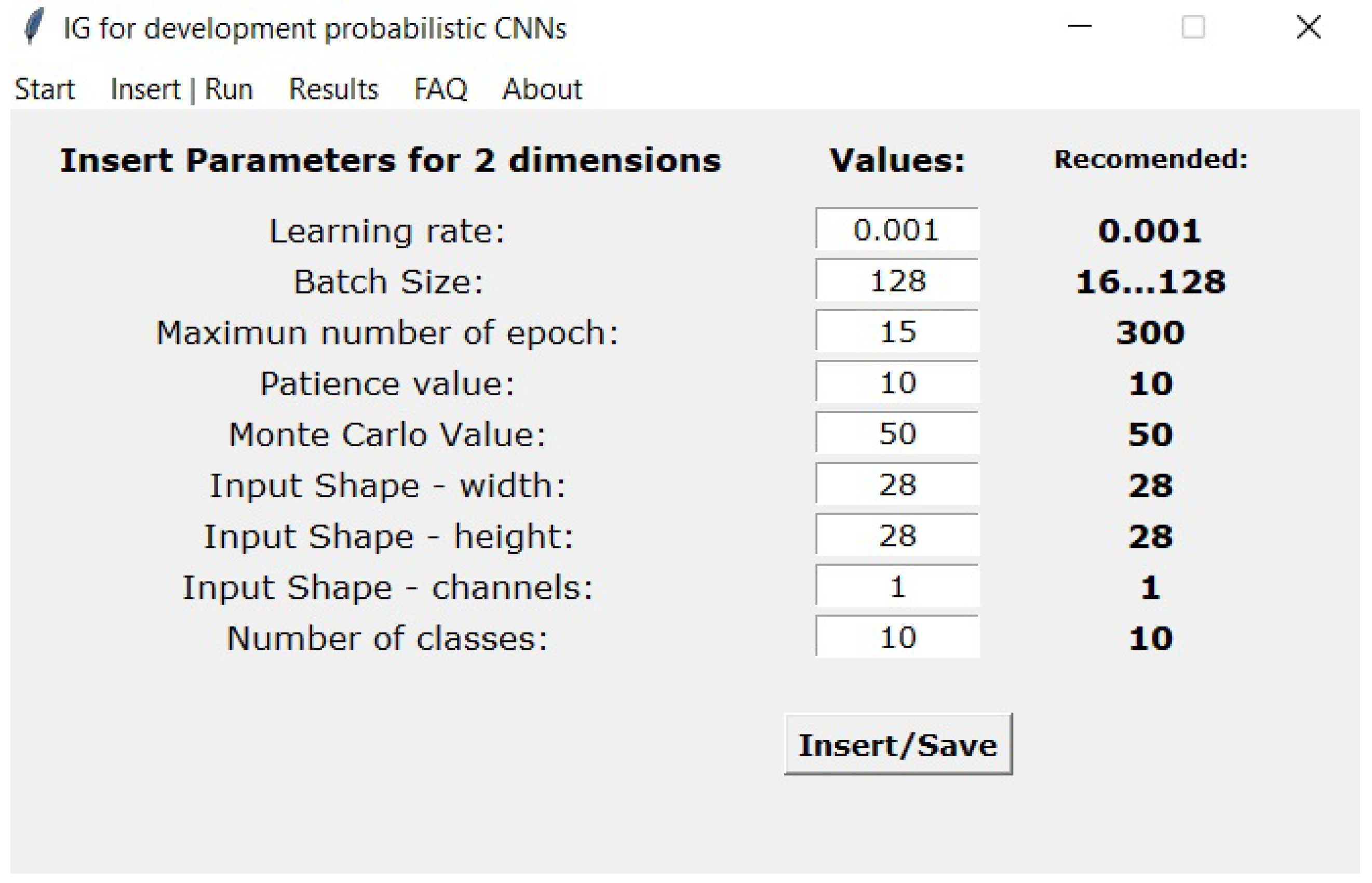
The GUI was tested for performing classification and regression tasks with one- and two-dimensional data. The first example to illustrate the GUI procedures is composed of a model for two-dimensional classification. Specifically, image data of hand-drawn numbers (MNIST dataset) were used (available at
http://yann.lecun.com/exdb/mnist, accessed on 2 February 2023). For this purpose, the standard LeNet-5 model (available at the GUI), with the default GUI options, was used as presented in
Figure 14. It is important to highlight that the purpose of the next examples is to show the use of the developed GUI and not the performance of the models used here as examples.
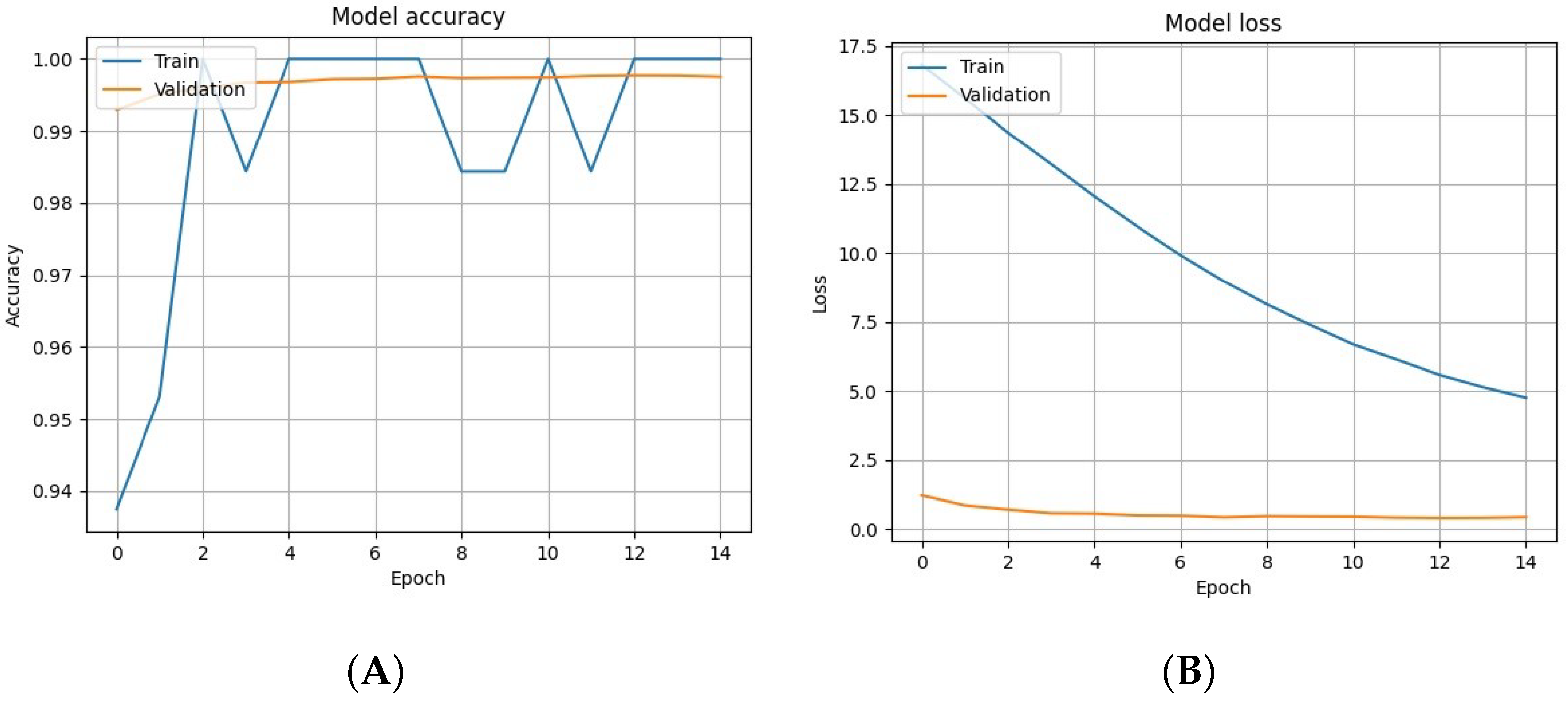
After training the LeNet-5 model, the following results are obtained at the model output:
Model’s training error, shown on the right side of
Figure 15.
Performance metrics, such as accuracy presented on the left side of
Figure 15.
Model’s epistemic uncertainty, shown in
Figure 17.
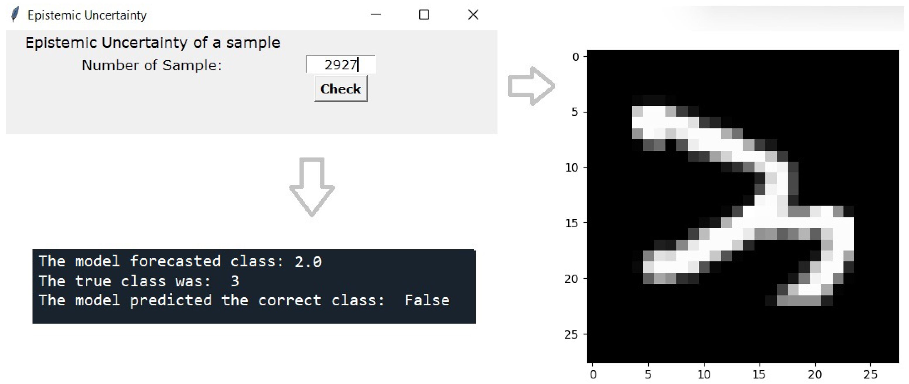
The window where it is possible to select a specific sample to visualize it (allowing, for example, to check a sample that was misclassified), shown in
Figure 18.
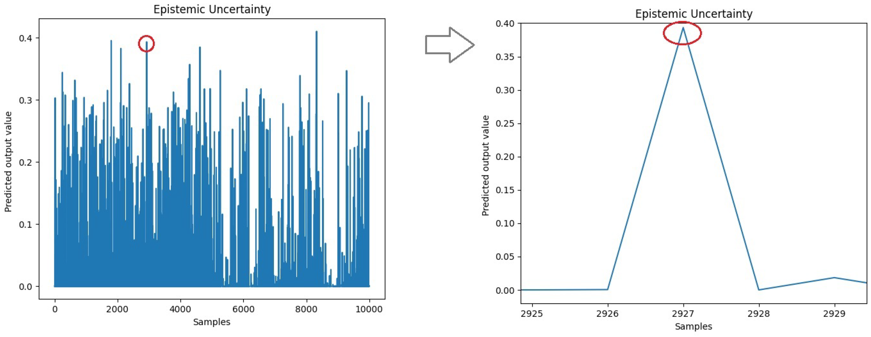
On the left side of
Figure 17, the epistemic uncertainty of the trained model is presented. In this example, one of the points where the uncertainty is higher is chosen, and on the right side, a zoom is performed to identify the sample number. After attaining the sample number, it can then be further analyzed as presented in
Figure 18. Pressing the “Check” button the sample is presented. Through IPython, it is possible to check into which class the model classified the sample, what was its true class, and the result of the model classification. It is possible to observe that the model classified the sample number 2927 as class 2. Its true class was 3, that is, the model failed to classify the sample correctly. Finally, in
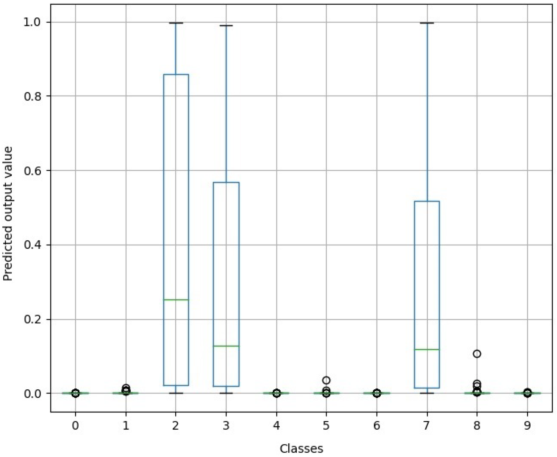
Figure 19, the epistemic uncertainty distributed over the various classes is shown.
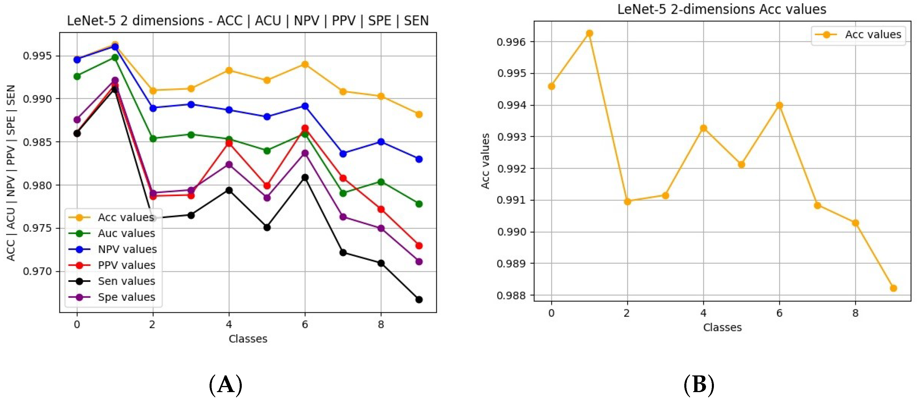
In the “Results” tab, pressing “See all the results in a plot” displays a single plot in a new window with the most relevant classification performance metrics: accuracy (Acc); area under the receiver operating characteristic curve (AUC); negative predictive value (NPV); positive predictive value (PPV); sensitivity (Sen); specificity (Spe).
The obtained results are shown on the left in
Figure 20. The user can select to view only one performance metric to ease the interpretation, as depicted on the right side of
Figure 21, where only Acc is shown. In the same tab, pressing “Print each result in IPython” prints the values of the chosen result on the IPython console.
All trained models and results are saved in a local folder, allowing the user to retrieve them for further use on other applications. The user can also resume training on a previously trained model and can perform transfer learning by loading a previously trained model and then retraining it on data from another problem.
The subsequent examination was performed on a regression test, where the goal was to determine the house prices in a Boston suburb or town using a standard dataset (Boston housing dataset, available at
https://www.cs.toronto.edu/~delve/data/boston/bostonDetail.html, accessed on 2 February 2023), using 14 features to feed the model. For this purpose, the LeNet-4 architecture was built using the custom model creation option (layer-by-layer specification).
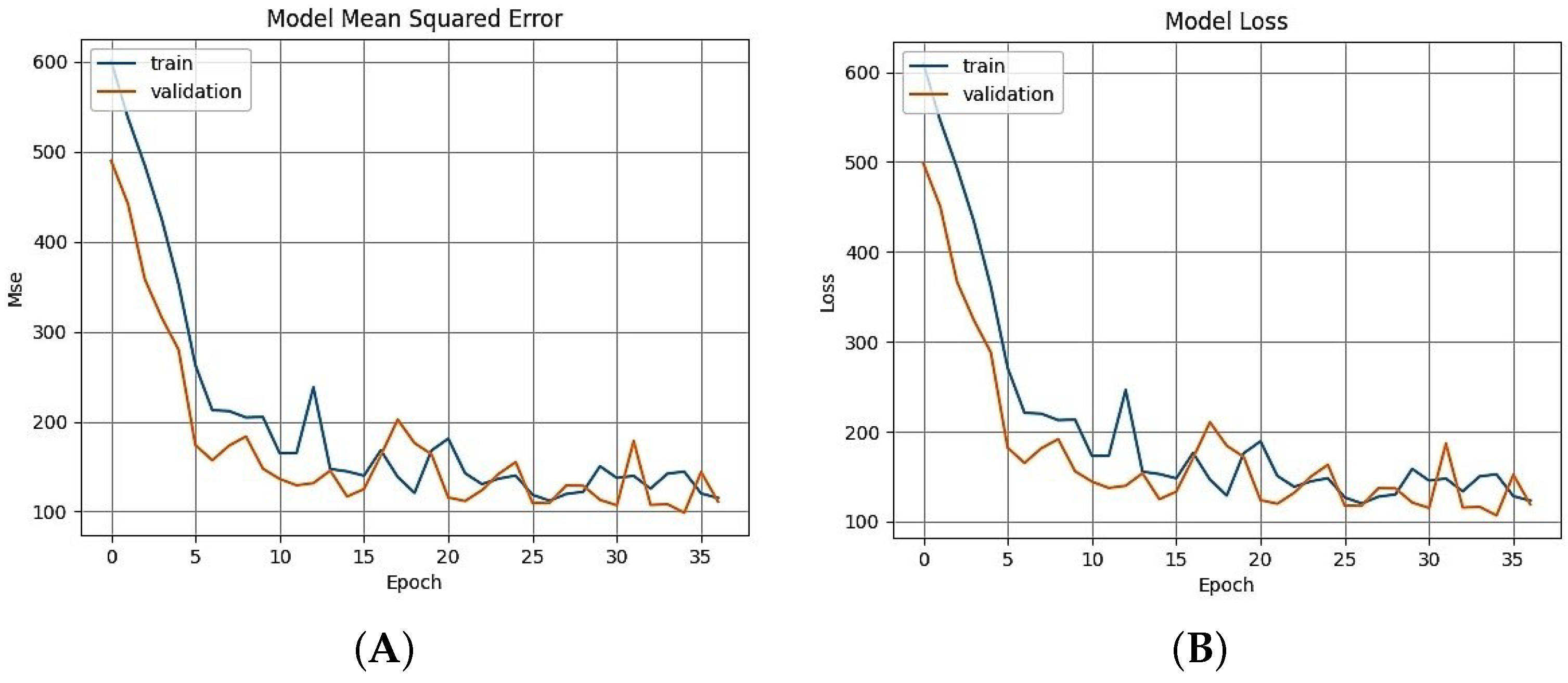
The training performance is presented to the user as shown in the example of
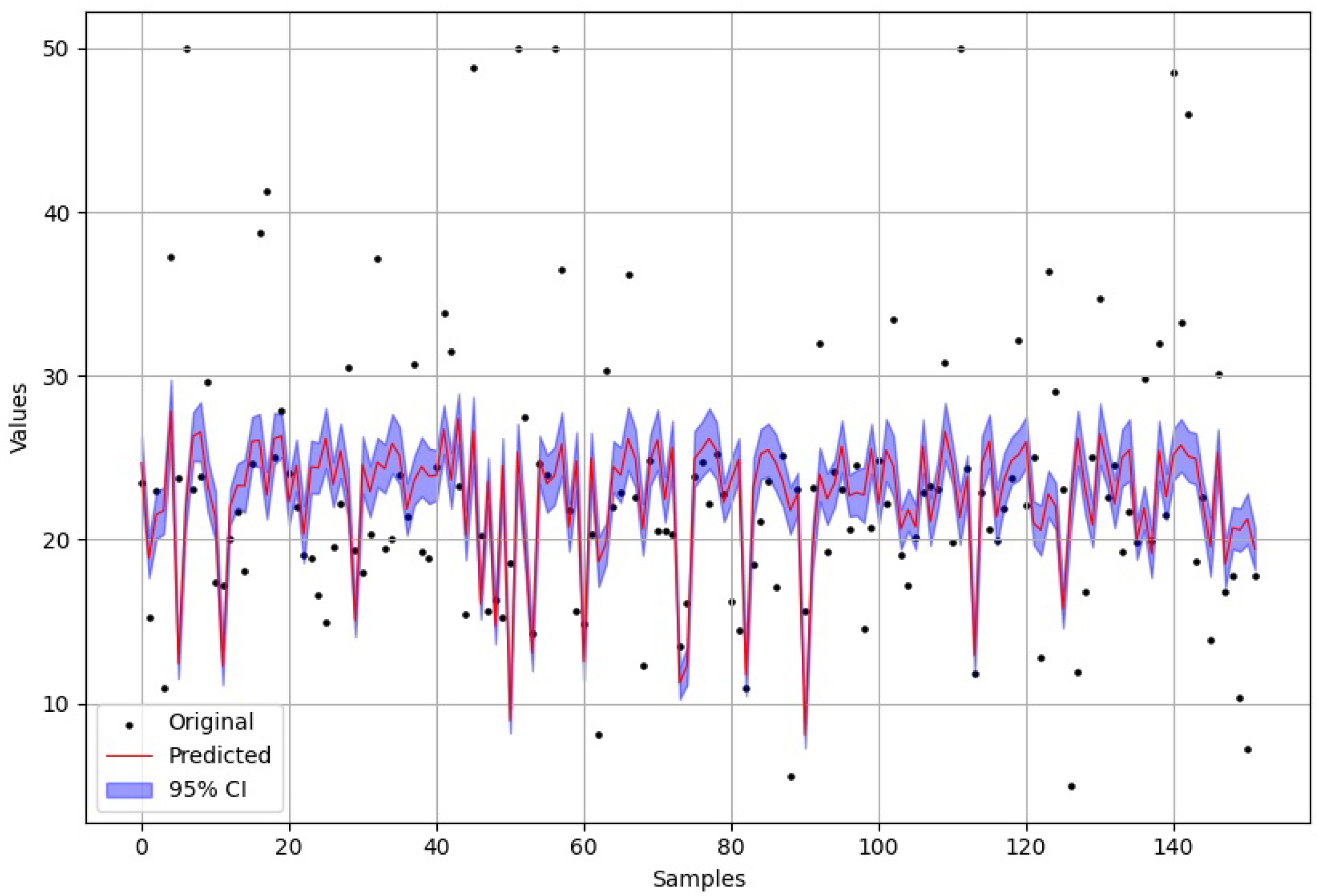
Figure 22. Furthermore, the test data predictions are also presented to the user. The PM also allows presenting the 95% confidence interval, as depicted in
Figure 23, allowing the user to clearly identify where the model is confident enough on its forecasts.
5. Conclusions
This work presents a graphical user interface for the development of probabilistic CNNs. This type of model can express epistemic uncertainty, a characteristic that is of great importance since it indicates the level of confidence the model has in its predictions. For instance, in medical fields where the outcome of the decision can affect the diagnosis, knowing the confidence level in the forecast is critical. Through the developed tool, it is possible to build PMs in a no-code approach without requiring in-depth knowledge in the domain of DL with probabilistic models, potentially speeding the development of applications where PMs are necessary. To the best of the author’s knowledge, no previous work has provided an interface for PMs, not even in the most popular platforms, such as Matlab Classification Learner (which conceptually is the closest to this work), Orange Data Mining, Rapid Miner, or Dataiku, making a direct comparison unfeasible. Furthermore, the developed tool employs a GUI that was shown, in usability tests, to be easy to use and capable of addressing the needs of users who want to develop probabilistic CNNs in a simple and straightforward way.
The implemented approach allows the user to either use standard architectures (already adapted for implementing a PM) for the model or to create a custom model, having the three most common layers (convolution, pooling, and dense) in DL available. Furthermore, the tool is fully adaptable and, if needed, the user can add or edit elements to it, including new standard models, performance metrics, and visualization methods.
The proposed tool was designed to allow the user to develop and test the models, requiring only to load the data (or use the standard datasets available in the tool’s database), select or specify the architecture, initiate the training, and then check the test results. The support documentation instructs the inexperienced user on how to use the tool, and the trained models are saved in a standard format, allowing the user to further use them on other applications. The following main paths are proposed as future steps in this research: the first is to implement a web-based version of the tool, allowing the back end to be run on a server while the front end can be executed on a browser; and the second path is to further expand the data visualization resources, allowing the user to carry out exploratory data analysis before starting the model development. Regarding the subsequent improvements, it is intended to add full support for cross validation. It can be done with the current version, but it requires the user to prepare the datasets outside of the developed tool.
Author Contributions
Conceptualization, A.C. and F.M.; methodology, A.C., F.M., S.S.M. and F.M.-D.; software, A.C. and F.M.; validation, F.M., S.S.M. and F.M.-D.; formal analysis, A.C., F.M., S.S.M. and F.M.-D.; investigation, A.C., F.M., S.S.M. and F.M.-D.; resources, F.M. and F.M.-D.; data curation, A.C. and F.M.; writing—original draft preparation, A.C. and F.M.; writing—review and editing, F.M., S.S.M. and F.M.-D.; visualization, A.C.; supervision, F.M. and F.M.-D.; project administration, F.M.-D.; funding acquisition, F.M.-D. All authors have read and agreed to the published version of the manuscript.
Funding
This research was funded by ARDITI—Agência Regional para o Desenvolvimento da Investi-gação, Tecnologia e Inovação under the scope of the project M1420-09-5369-FSE-000002—Post-Doctoral Fellowship, co-financed by the Madeira 14-20 Program—European Social Fund. This research was funded by LARSyS (Project UIDB/50009/2020).
Data Availability Statement
Not applicable.
Conflicts of Interest
The authors declare no conflict of interest.
Abbreviations
The following abbreviations are used in this manuscript:
| AI | Artificial Intelligence |
| ML | Machine Learning |
| ANN | Artificial Neural Networks |
| DL | Deep Learning |
| CNN | Convolutional Neural Network |
| GPU | Graphics Processing Units |
| TF | TensorFlow |
| PM | Probabilistic Model |
| VI | Variational Inference |
| DM | Deterministic Model |
| GUI | Graphical User Interface |
| CUDA | Compute Unified Device Architecture Architecture |
| AF | Activation Function |
| ReLU | Rectified Linear Unit |
| PM | Probabilistic Model |
| Acc | Accuracy |
| AUC | Area Under the Receiver Operating Characteristic Curve |
| KLD | Kullback–Leibler Divergence |
| NPV | Negative Predictive Value |
| PPV | Positive Predictive Value |
| Sen | Sensitivity |
| CSV | Comma-Separated Values |
| Spe | Specificity |
References
- Hamet, P.; Tremblay, J. Artificial intelligence in medicine. Metabolism 2017, 69, S36–S40. [Google Scholar] [CrossRef] [PubMed]
- Carleo, G.; Cirac, I.; Cranmer, K.; Daudet, L.; Schuld, M.; Tishby, N.; VogtMaranto, L.; Zdeborova, L. Machine learning and the physical sciences. Rev. Mod. Phys. 2019, 91, 045002. [Google Scholar] [CrossRef]
- LeCun, Y.; Bengio, Y.; Hinton, G. Deep learning. Nature 2015, 521, 436–444. [Google Scholar] [CrossRef] [PubMed]
- Ravindra, S. How Convolutional Neural Networks Accomplish Image Recognition. 2017. Available online: https://medium.com/@savaramravindra4/howconvolutional-neural-networks-accomplish-image-recognition-277033b72436 (accessed on 15 December 2022).
- Falcão, J.V.R.; Moreira, V.; Santos, F.; Ramos, C. Redes Neurais Deep Learning Com Tensorflow. 2019. Available online: https://revistas.unifenas.br/index.php/RE3C/article/view/232 (accessed on 4 January 2023).
- Moolayil, J. An introduction to deep learning and keras. In Learn Keras for Deep Neural Networks; Springer: Berlin, Germany, 2019; pp. 1–16. [Google Scholar]
- Shridhar, K.; Laumann, F.; Liwicki, M. A comprehensive guide to bayesian convolutional neural network with variational inference. arXiv 2019, arXiv:1901.02731. [Google Scholar]
- Durr, O.; Sick, B.; Murina, E. Probabilistic Deep Learning: With Python, Keras and Tensorflow Probability; Manning Publications: New York, NY, USA, 2020. [Google Scholar]
- Etter, D.M.; Kuncicky, D.C.; Hull, D.W. Introduction to MATLAB; Prentice Hall: Hoboken, NJ, USA, 2002. [Google Scholar]
- Demsar, J.; Curk, T.; Erjavec, A.; Gorup, C.; Hocevar, T.; Milutinovic, M.; Movina, M.; Polajnar, M.; Toplak, M.; Staric, A.; et al. Orange: Data mining toolbox in python. J. Mach. Learn. Res. 2013, 14, 2349–2353. [Google Scholar]
- Bisong, E. Python. In Building Machine Learning and Deep Learning Models on Google Cloud Platform; Springer: Berlin, Germany, 2019; pp. 71–89. [Google Scholar]
- Beniz, D.; Espindola, A. Using tkinter of python to create graphical user interface (GUI) for scripts in lnls. WEPOPRPO25 2016, 9, 25–28. [Google Scholar]
- Mocanu, I. An introduction to cuda programming. J. Inf. Syst. Oper. Manag. 2008, 2, 495–506. [Google Scholar]
- Mahajan, P.; Abrol, P.; Lehana, P.K. Scene based classification of aerial images using convolution neural networks. J. Sci. Ind. Res. (JSIR) 2020, 79, 1087–1094. [Google Scholar]
- Liu, Y.; Starzyk, J.A.; Zhu, Z. Optimized approximation algorithm in neural networks without overfitting. IEEE Trans. Neural Netw. 2008, 19, 983–995. [Google Scholar] [PubMed]
- Blei, D.M.; Kucukelbir, A.; McAuliffe, J.D. Variational inference: A review for statisticians. J. Am. Stat. Assoc. 2017, 112, 859–877. [Google Scholar] [CrossRef]
- Erven, T.V.; Harremos, P. Renyi divergence and kullback-leibler divergence. IEEE Trans. Inf. Theory 2014, 60, 3797–3820. [Google Scholar] [CrossRef]
- Queiroz, R.B.; Rodrigues, A.G.; Gomez, A.T. Estudo comparativo entre as técnicas máxima verossimilhança gaussiana e redes neurais na classificação de imagens ir-mss cbers 1. In I WorkComp Sul; 2004; Volume 1, Available online: https://www.academia.edu/1099155/Estudo_comparativo_entre_as_t%C3%A9cnicas_m%C3%A1xima_verossimilhan%C3%A7a_gaussiana_e_redes_neurais_na_classifica%C3%A7%C3%A3o_de_imagens_IR_MSS_CBERS_1 (accessed on 2 February 2023).
- Wen, Y.; Vicol, P.; Ba, J.; Tran, D.; Grosse, R. Flipout: Efficient pseudo-independent weight perturbations on mini-batches. arXiv 2018, arXiv:1803.04386. [Google Scholar]
- Shridhar, K.; Laumann, F.; Liwicki, M. Uncertainty estimations by softplus normalization in bayesian convolutional neural networks with variational inference. arXiv 2018, arXiv:1806.05978. [Google Scholar]
- Gutiérrez-Carreón, G.; Daradoumis, T.; Esteve, J. Integrating learning services in the cloud: An approach that benefits both systems and learning. J. Educ. Technol. Soc. 2015, 18, 145–157. [Google Scholar]
Figure 1.
Developed graphical user interface tabs.
Figure 1.
Developed graphical user interface tabs.
Figure 2.
“Start” tab, showing the steps for using the GUI for all data sets.
Figure 2.
“Start” tab, showing the steps for using the GUI for all data sets.
Figure 3.
Folder organization of the developed GUI, where the user should save the data with the indicated names of the example, and the results folder will save all outputs of the trained model (each model is saved in a different folder).
Figure 3.
Folder organization of the developed GUI, where the user should save the data with the indicated names of the example, and the results folder will save all outputs of the trained model (each model is saved in a different folder).
Figure 4.
Menu for adding the parameters of the GUI, separator “Insert|Run”, for the (A) one-dimensional and (B) two-dimensional data.
Figure 4.
Menu for adding the parameters of the GUI, separator “Insert|Run”, for the (A) one-dimensional and (B) two-dimensional data.
Figure 5.
IPython console displaying the confirmation of chosen parameters.
Figure 5.
IPython console displaying the confirmation of chosen parameters.
Figure 6.
Tab “Insert|Run”, displayed after inserting parameters.
Figure 6.
Tab “Insert|Run”, displayed after inserting parameters.
Figure 7.
IPython console with information on the training progress of the model.
Figure 7.
IPython console with information on the training progress of the model.
Figure 8.
Creation of a custom model by choosing the sequence of its composing layers.
Figure 8.
Creation of a custom model by choosing the sequence of its composing layers.
Figure 9.
Presentation of the “Results” tab.
Figure 9.
Presentation of the “Results” tab.
Figure 10.
Depiction of the “FAQ“ tab, showing the required modules/libraries and the button for viewing the videos.
Figure 10.
Depiction of the “FAQ“ tab, showing the required modules/libraries and the button for viewing the videos.
Figure 11.
Presentation of the “About“ tab.
Figure 11.
Presentation of the “About“ tab.
Figure 12.
Navigation map developed for the GUI.
Figure 12.
Navigation map developed for the GUI.
Figure 13.
Low- and high-fidelity prototypes developed for the GUI.
Figure 13.
Low- and high-fidelity prototypes developed for the GUI.
Figure 14.
Parameters used for the LeNet-5 model for the two-dimensional dataset (MNIST).
Figure 14.
Parameters used for the LeNet-5 model for the two-dimensional dataset (MNIST).
Figure 15.
Example of the attained (A) test accuracy and (B) training error for the LeNet-5 model, trained on a two-dimensional dataset (MNIST).
Figure 15.
Example of the attained (A) test accuracy and (B) training error for the LeNet-5 model, trained on a two-dimensional dataset (MNIST).
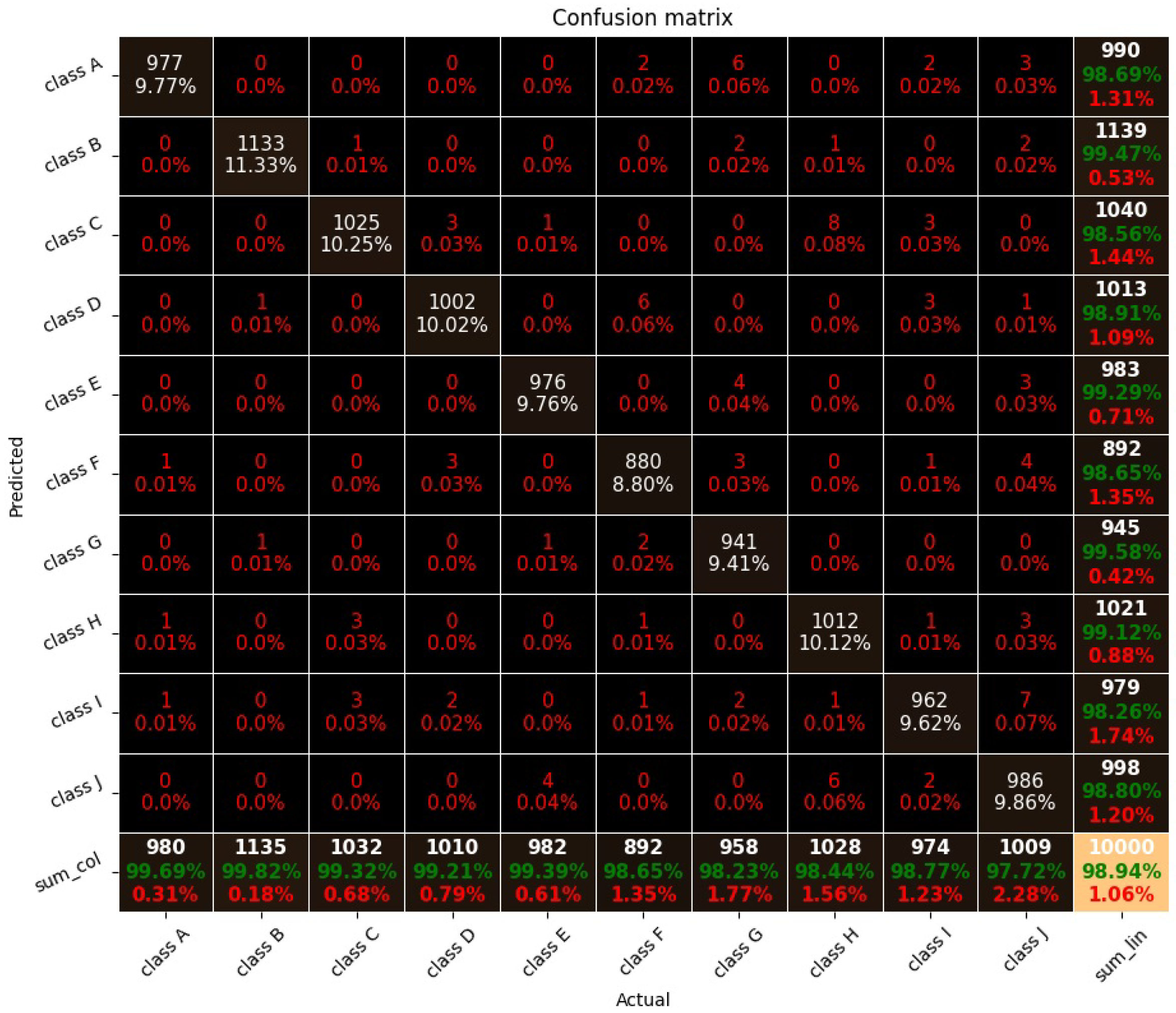
Figure 16.
Confusion matrix for the LeNet-5 model, trained on a two-dimensional dataset (MNIST). Correct (in green) and wrong (in red).
Figure 16.
Confusion matrix for the LeNet-5 model, trained on a two-dimensional dataset (MNIST). Correct (in green) and wrong (in red).
Figure 17.
Example of the test data epistemic uncertainty from a trained model, where a high uncertainty sample (number 2927) is highlighted in the left panel, and then a zoom is performed in the right panel to further show the sample’s amplitude.
Figure 17.
Example of the test data epistemic uncertainty from a trained model, where a high uncertainty sample (number 2927) is highlighted in the left panel, and then a zoom is performed in the right panel to further show the sample’s amplitude.
Figure 18.
Analysis of sample number 2927 from the presented example, showing the sample’s image on the right panel and the model output on the bottom panel.
Figure 18.
Analysis of sample number 2927 from the presented example, showing the sample’s image on the right panel and the model output on the bottom panel.
Figure 19.
Epistemic uncertainty distributed across the various classes, relative to the LeNet-5 model for the two-dimensional dataset (MNIST). The green line is the median of the class data.
Figure 19.
Epistemic uncertainty distributed across the various classes, relative to the LeNet-5 model for the two-dimensional dataset (MNIST). The green line is the median of the class data.
Figure 20.
Performance metrics presented when choosing “Print each result in IPython” for the example using LeNet-5 model for the two-dimensional dataset (MNIST).
Figure 20.
Performance metrics presented when choosing “Print each result in IPython” for the example using LeNet-5 model for the two-dimensional dataset (MNIST).
Figure 21.
Example of the plots depicted when choosing (A) “See all the results in a plot” and (B) “See each result in a plot”, relative to the example using the LeNet-5 model for the two-dimensional dataset (MNIST).
Figure 21.
Example of the plots depicted when choosing (A) “See all the results in a plot” and (B) “See each result in a plot”, relative to the example using the LeNet-5 model for the two-dimensional dataset (MNIST).
Figure 22.
Performance of the regression model (LeNet-4 created using the layer-by-layer creation option) during training using a standard regression dataset (Boston housing), presenting the estimated (A) mean squared error and (B) loss.
Figure 22.
Performance of the regression model (LeNet-4 created using the layer-by-layer creation option) during training using a standard regression dataset (Boston housing), presenting the estimated (A) mean squared error and (B) loss.
Figure 23.
Forecasts of the regression model (LeNet-4 created using the layer-by-layer creation option) in the test data training using a standard regression dataset (Boston housing), where the 95% confidence interval is presented.
Figure 23.
Forecasts of the regression model (LeNet-4 created using the layer-by-layer creation option) in the test data training using a standard regression dataset (Boston housing), where the 95% confidence interval is presented.
| Disclaimer/Publisher’s Note: The statements, opinions and data contained in all publications are solely those of the individual author(s) and contributor(s) and not of MDPI and/or the editor(s). MDPI and/or the editor(s) disclaim responsibility for any injury to people or property resulting from any ideas, methods, instructions or products referred to in the content. |
© 2023 by the authors. Licensee MDPI, Basel, Switzerland. This article is an open access article distributed under the terms and conditions of the Creative Commons Attribution (CC BY) license (https://creativecommons.org/licenses/by/4.0/).


 ,
, 


