An Investigation into the Physical Mechanisms of Leak Noise Propagation in Buried Plastic Water Pipes: A Wave Dynamic Stiffness Approach

Abstract

In buried plastic water pipes, the predominantly fluid-borne wave is of particular interest, as it plays a key role in the propagation of leak noise. Consequently, it has been studied by several researchers to determine the speed of wave propagation and its attenuation with distance. These features are encapsulated in the wavenumber. By examining the factors that govern the behaviour of this wavenumber, this paper presents an in-depth examination of the physical mechanisms of leak noise propagation. To achieve this, an alternative physics-based model for the wavenumber is developed, using the concept of the wave dynamic stiffnesses of the individual components within the pipe system, i.e., the water in the pipe, the pipe wall, and the surrounding medium. This facilitates a clear interpretation of the wave behaviour in terms of the physical properties of the system, especially the interface between the pipe and the surrounding medium, which can have a profound influence on the leakage of acoustic energy from the pipe wall into the external medium. Three systems with different types of surrounding medium are studied, and the factors that govern leak noise propagation in each case are identified. Experimental results on two distinct test sites from different parts of the world are provided to validate the approach using leak noise as an excitation mechanism.

1. Introduction

Pipelines are crucial elements in many engineering systems and are widely used to transport water [1,2]. However, the efficiency of these systems can be compromised by issues such as water leaks [3,4]. When undetected or neglected, these leaks can lead to significant wastage of water, posing both environmental and economic challenges across the world [5,6,7]. In 2019, the European Environmental Agency reported that water scarcity impacted 29% of the EU territory for at least one season [8]. Furthermore, it is estimated that about 23% of drinking water in Europe is lost on average [9]. Meanwhile, in Brazil, the average water loss is around 38%, with eight states experiencing even more alarming losses exceeding 50%, such as the Roraima state, in which the loss is about 75% [10].

The modelling of wave propagation in buried water pipes is particularly important for the water industry, as they search for ways to improve leak detection technology [11,12,13]. In buried plastic water distribution pipes, leak noise propagates as a predominantly fluid-borne (s = 1) wave [14,15]. This is an axisymmetric (n = 0) wave, where the acoustic pressure of the water is strongly coupled to the vibrations of the pipe wall [16]. The wave involves a large radial motion of the pipe wall and an axial plane wave motion of the water. At frequencies much lower than the ring frequency of the pipe [15], the other axisymmetric structural-acoustic wave is the (s = 2) wave, which is a predominantly structure-borne wave. However, this wave tends not to be strongly excited by a leak, which generates an oscillating pressure inside the pipe due to turbulence as the water escapes from the pipe. Thus, the focus of this paper is the predominantly fluid-borne wave, a graphical description of which can be found in a webinar by the International Water Association Water Loss Specialist Group [17].

The detection and localization of water leaks via vibro-acoustic methods, such as acoustic correlators [18], rely primarily on the time delay estimation technique [19,20], which depends heavily on the way in which leak noise propagates. To determine the way in which this is affected by the properties of the pipe and the surrounding medium, a model is needed. Modelling wave propagation in buried plastic pipes is more challenging than for metal pipes because of the high degree of dynamic coupling between the water, the plastic pipe wall, and the surrounding soil. These effects need to be appropriately modelled to ensure that accurate predictions can be made of the speed and attenuation of leak noise propagation. Although there is water–pipe–soil coupling in metal pipes, in general, it is much less than for a plastic pipe, due to the much higher hoop stiffness of metal pipes used in water distribution systems. Much research on wave propagation in fluid-filled pipes has been carried out hitherto. Fuller and Fahy [21] determined the propagation characteristics of axisymmetric waves and the dispersion curves of thin-walled pipes in vacuo filled with ideal fluid using the Donnel–Mushtari shell theory. The authors also investigated how the vibrational energy in the pipe wall and the fluid within the pipe changes with frequency. In 1994, Pinnington and Briscoe [14] determined approximate analytical expressions for the two wavenumbers (s = 1, 2) for an in vacuo fluid-filled pipe. Unlike previous work, their analysis was confined to frequencies well below the ring frequency of the pipe and was the basis for the later work by researchers on leak detection in water-filled plastic pipes. Xu and Zhang [22] studied the vibrational energy flow input from an external force as well as the transmission along the shell. The authors found that the input power flow, as well as the power flow transmitted along the shell, depends highly upon the characteristics of the waveforms travelling in the pipe wall. Sinha et al. [23] investigated the axisymmetric motion of submerged fluid-filled pipes and determined which modes leak energy into the surrounding fluid. Pan et al. [24] studied axisymmetric acoustic wave propagation in a fluid-filled pipe with arbitrary thickness both experimentally and numerically. A few years later, Prek [25] experimentally investigated a frequency domain method for the determination of wave propagation characteristics in fluid-filled viscoelastic pipes, using different pipe wall materials. The authors carried out complex wavenumber estimation using hydrophones.

Some researchers have also focused on the wave characteristics of fluid-filled pipes buried in soil. Long et al. [26] studied the axisymmetric wave modes propagating in buried iron fluid-filled pipes, predicting the corresponding phase velocity. Further, Long et al. [27] studied the attenuation of some waves that propagate in buried iron water pipes. Deng and Yang [28] adopted the Flügge shell theory to model a pipe and the Winkler model for the surrounding soil. The authors studied the effects of wall thickness, the elastic properties of the soil, and the fluid velocity variations. Leinov et al. [29] conducted some laboratory tests involving the propagation of guided waves in a carbon steel pipe buried in sand. The authors investigated the attenuation properties of the waves for various sand conditions including loose, compacted, mechanically compacted, water-saturated, and drained.

Building on the work of Pinnington and Briscoe [14,15], Muggleton et al. [16] developed an analytical model to predict both the wave speed and attenuation of a buried water-filled plastic pipe. The soil was treated as a fluid supporting two different waves, each of which exerted normal dynamic pressure on the pipe wall. Although the shear coupling of the pipe to the surrounding soil was not properly accounted for, the theoretical and experimental results showed good agreement at low frequencies. The soil properties were then modelled more effectively in the subsequent work of Muggleton and Yan [30], in which the soil was coupled to the pipe in the radial direction but not in the axial direction. In this case, there is a lubricated contact between the pipe wall and the surrounding soil. The authors derived wavenumbers for the two coupled axisymmetric waves (s = 1 and s = 2) and showed that the shear modulus of the soil is an important parameter, influencing the speed of the predominantly fluid-borne wave. A couple of years later, Yan and Zhang [31] studied the low-frequency acoustic characteristics of propagation and attenuation of the (s = 1 and s = 2) waves in immersed pipes conveying fluid. They investigated the influence of material properties and the effects of shell thickness/radius ratio as well as the density of the contained fluid.

In 2018, Brennan et al. [32] compared the analytical model to predict the wavenumber of the s = 1 under a lubricated contact between the pipe wall and the soil, with a finite element model of the water–pipe–soil system, and some experimental results from different test sites. The authors validated the conclusions found in [30] concerning the importance of the shear modulus of the soil on the speed of the predominantly fluid-borne wave. Gao et al. [33] proposed a more complete model to predict the relationships for the predominantly fluid-borne wave. In this model, the pipe is connected to the soil both radially and axially with perfect bonding at the pipe–soil interface. It was found that the surrounding medium effectively adds mass to the pipe wall, whereas the shear properties of the soil effectively add stiffness. The model described in [33] was further adapted by Liu et al. [34] to investigate vibro-acoustic propagation in buried gas pipes. They proposed an effective radiation coefficient to measure the radiation of the gas-dominated and shell-dominated waves. Wang et al. [35] investigated the wave characteristics of buried water pipes considering the viscosity and fluid flow using a model derived from Love’s thin shell theory. Investigations were carried out by analyzing the effect of different types of soil and pipes and showed that a viscous fluid causes greater wave attenuation compared to an ideal fluid.

For the purposes of studying buried water plastic pipes in the context of water leak detection, the model developed in [33] is considered to be the most complete. This paper builds on the work described in these articles. The aim is to present a comprehensive investigation into the physical mechanisms governing leak noise propagation. To achieve this, and especially to determine the role of the interface between the pipe and the surrounding medium, the model from [33] is reformulated in terms of the wave dynamic stiffnesses, namely the pipe, the water, and the surrounding medium. It is believed that such an investigation, which assimilates much of the previous work in a convenient and physically interpretable form, has not been carried out before. At the core of the model is the wavenumber of the predominantly fluid-borne wave, which is written in terms of the wave dynamic stiffnesses. To validate the model, some experimental results are presented on the measurement of the real and imaginary parts of the wavenumber from two sites in which a plastic water pipe is buried in sandy and clay soil, respectively. In both cases, the pipe vibration is generated by a leak.

The paper is organised as follows. Following the introduction, in Section 2, the objectives of the paper are defined, as are the assumptions made in the derivation of the wavenumber for the predominantly fluid-borne wave. Section 3 describes the derivation of the wavenumber as a function of wave dynamic stiffness matrices of the component parts of the system. Some experimental work to validate the wave dynamic stiffness approach is carried out in Section 4. The dynamic stiffnesses of the component parts are presented for three types of surrounding medium in Section 5 and their physical significance is discussed. The influences of the various parts of the system on the propagation characteristics of the predominantly fluid-borne wave are discussed in Section 6, and some conclusions are given in Section 7. There is also an Appendix, which shows how the lubricated interface between the pipe and soil can be described using the proposed model.

2. Problem Statement

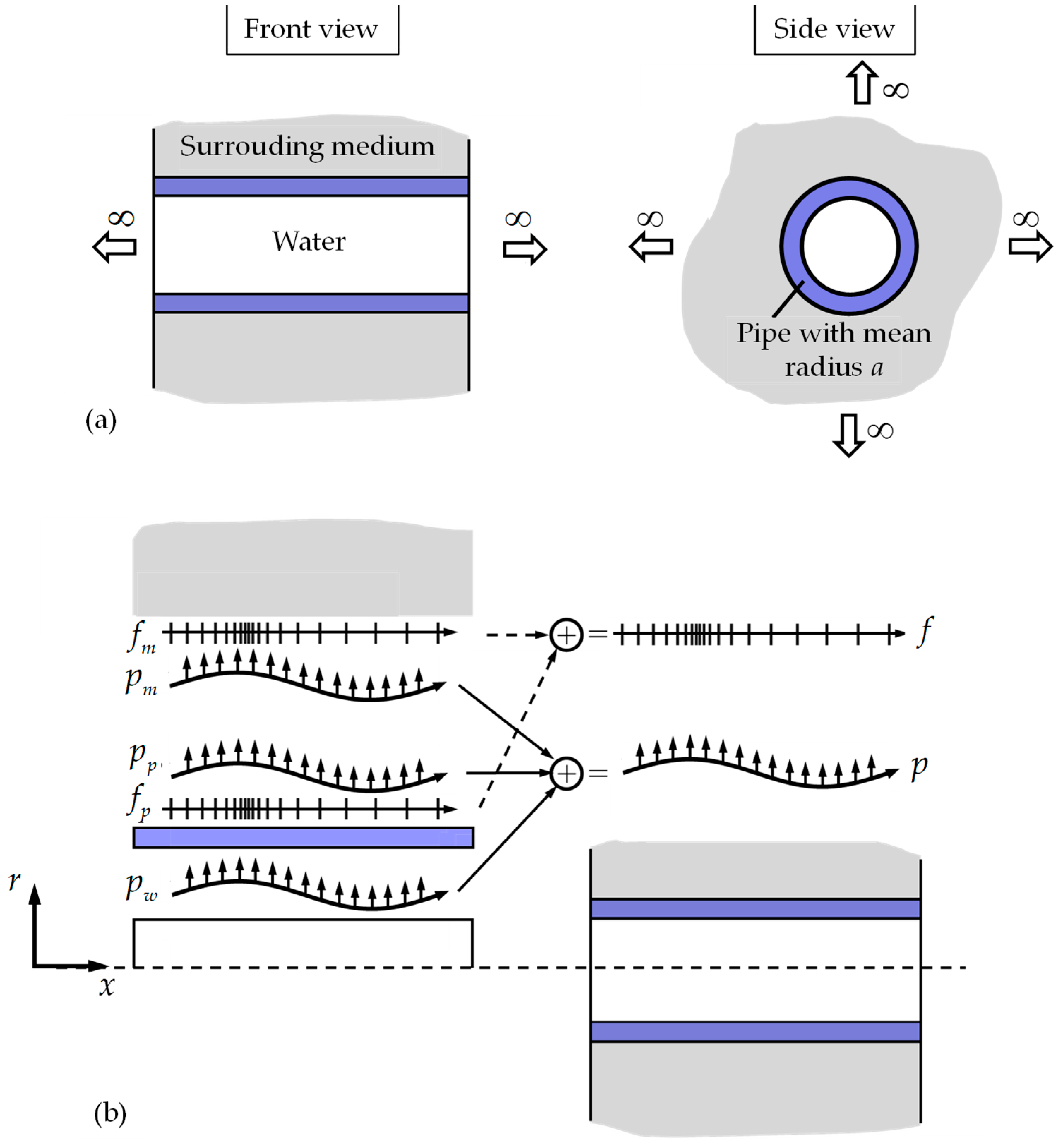
The water-filled pipe surrounded by an external medium of interest is shown in Figure 1a. The external medium can be either water or soil. The pipe has a mean radius a and wall thickness h.

Of interest in this paper is the way in which the pipe material and its geometry, along with the soil properties, affect noise propagation from a leak to a measurement point. Of particular interest is the effect of the axial coupling between the pipe and its surrounding medium and how this influences the radiation of acoustic leakage energy into the surrounding medium. To achieve this, an analytical model of the wavenumber is required, and in this paper, this is derived as a function of the wave dynamic stiffnesses of the component parts of the system, i.e., the water in the pipe, the pipe wall, and the surrounding medium. By focusing on wave dynamic stiffnesses, it is possible to identify and assess the specific contribution of each part. Wave dynamic stiffness is similar in concept to wave impedance described by Fahy and Gardonio [36], but rather than using the variables of force (or pressure) and velocity, displacement is used instead of velocity, as this is more convenient for the model of the pipe system since the displacement of the pipe wall is directly proportional to the acoustic pressure. The result is a more compact and elegant model with less complicated algebraic expressions. It essentially involves a pressure that is harmonic in both space and time being applied to a structure or a fluid. For an arbitrary one-dimensional structure in the x direction, which has a wavenumber k, this could be $p=P\exp \left(\mathrm{j}\left(\omega t-kx\right)\right)$, where $\omega$ is the circular frequency and $\mathrm{j}=\sqrt{-1}.$ The response is then described by $v=V\exp \left(\mathrm{j}\left(\omega t-kx\right)\right)$, since the structure/fluid is considered to be linear. The wave dynamic stiffness is defined as the ratio $K\left(\omega ,k\right)=P\left(\omega ,k\right)/V\left(\omega ,k\right),$ i.e., it is a complex quantity that is dependent on both the frequency and wavenumber. The real part of the wave dynamic stiffness is related to the stiffness or inertial properties of the system and the imaginary part of the wave dynamic stiffness is related to energy dissipation.

The wavenumber of the predominantly fluid-borne wave is the key quantity that captures the way in which the leak noise propagates in the pipe, and is derived in the following section. The following simplifying assumptions are made:

• The pipe and surrounding medium are of infinite extent in the axial direction, and the surrounding medium is of infinite extent in the radial direction;
• The predominantly fluid-dominated axisymmetric wave is the only wave propagating in the pipe and is wholly responsible for the propagation of leak noise;
• The frequency range of interest is well below the pipe ring frequency, so that bending in the pipe wall is neglected. The ring frequency is the resonance frequency where the circumference is equal to one wavelength of a compressional wave in the pipe wall;
• The frequency range of interest is such that an acoustic wavelength of water is much greater than the diameter of the pipe.

In such a system, the frequency response function (FRF) between the acoustic pressure at an arbitrary position in the pipe and the acoustic pressure at another position d metres away is given by

$$H(\omega ,d)=\exp \left(-\mathrm{j}kd\right)$$

(1a)

which simply represents a decaying, predominantly fluid-borne, propagating wave. The wavenumber is complex, because the amplitude of the wave decreases as it propagates along the pipe. To clarify how the wavenumber is related to the physical behaviour of the wave, it is useful to rewrite Equation (1a) as [20]

$$H(\omega ,d)=\exp \left(-\omega \beta d\right)\exp \left(-\mathrm{j}\omega d/c\right)$$

(1b)

where $\beta =-\mathrm{Im}\left\{k\right\}/\omega ={\eta }_{\mathrm{wave}}/2c$ is a measure of the loss as the wave propagates along the pipe wall and $c=\omega /\mathrm{Re}\left\{k\right\}$ is the speed at which it propagates, and ${\eta }_{\mathrm{wave}}=-2\mathrm{Im}\left\{k\right\}/\mathrm{Re}\left\{k\right\}$ is defined as the loss factor. Thus, the two main features of the predominantly fluid-borne propagating wave, namely the speed at which it propagates and the amount it decays, are encapsulated in the wavenumber. The following sections show how the wavenumber is related to the pipe and soil properties in a clear physical way using the concept of wave dynamic stiffness. Three distinct scenarios are investigated involving water, clay soil, and sandy soil as the surrounding mediums and the governing factors influencing the leak noise propagation in each case are identified.

3. Derivation of the Wavenumber

The pipe system can be split into three components: the water within the pipe, the pipe wall, and the surrounding medium. This is shown in Figure 1b, in which the applied forces per unit area/pressures to each component are shown. Note that these are assumed to be harmonic in both space and time, i.e., $f_{p,m}=F_{p,m}\exp \left(\mathrm{j}\left(\omega t-kx\right)\right), p_{w,p,m}=P_{w,p,m}\exp \left(\mathrm{j}\left(\omega t-kx\right)\right),$ and the axial and radial displacements of the three components are given by $u_{p,m}=U_{p,m}\exp \left(\mathrm{j}\left(\omega t-kx\right)\right) \mathrm{and} w_{w,p,m}=W_{w,p,m}\exp \left(\mathrm{j}\left(\omega t-kx\right)\right)$, respectively. Radial pressures are applied to each component, but axial forces are only applied to the pipe and the external medium, as there is no axial reaction force between the water inside the pipe and the pipe wall. The frequency domain relationships between the forces per unit area/pressures and the axial and radial displacements for each of the three components are given by

$$P_w=K^{\left(\mathrm{water}\right)}{W}_w$$

(2a)

$$\left\{\begin{array}{c}{F}_p\\ P_p\end{array}\right\}=\left[\begin{array}{cc}{K}_{11}^{(\mathrm{pipe})}& K_{12}^{(\mathrm{pipe})}\\ K_{21}^{(\mathrm{pipe})}& K_{22}^{(\mathrm{pipe})}\end{array}\right]\left\{\begin{array}{c}{U}_p\\ W_p\end{array}\right\}$$

(2b)

$$\left\{\begin{array}{c}{F}_m\\ P_m\end{array}\right\}=\left[\begin{array}{cc}{K}_{11}^{(\mathrm{medium})}& K_{12}^{(\mathrm{medium})}\\ K_{21}^{(\mathrm{medium})}& K_{22}^{(\mathrm{medium})}\end{array}\right]\left\{\begin{array}{c}{U}_m\\ W_m\end{array}\right\}$$

(2c)

where the K’s are the wave dynamic stiffnesses of the component parts. Note that $F=F_p+F_m$ and $P=P_w+P_p+P_m,$ as the component parts, act in parallel so the applied force/pressure is shared between them. Note also that at the water/pipe/surrounding medium interface $W_w=W_p=W_m,$ so the combined system wave dynamic stiffness equation can be alternatively written as

$$p=\left[K^{\left(\mathrm{pipe}\right)}+K^{\left(\mathrm{water}\right)}+K^{\left(\mathrm{medium}\right)}\right]u$$

(3)

where $p={\left\{\begin{array}{cc}F& P\end{array}\right\}}^T, u=\left\{{\begin{array}{cc}{U}_p& W\end{array}}_p\right\},$ and $K^{\left(\mathrm{pipe}\right)}=\left[\begin{array}{cc}{K}_{11}^{(\mathrm{pipe})}& K_{12}^{(\mathrm{pipe})}\\ K_{21}^{(\mathrm{pipe})}& K_{22}^{(\mathrm{pipe})}\end{array}\right], K^{\left(\mathrm{water}\right)}=\left[\begin{array}{cc}0& 0\\ 0& K_{ }^{(\mathrm{water})}\end{array}\right]$, and $K^{\left(\mathrm{pipe}\right)}=\left[\begin{array}{cc}{K}_{11}^{(\mathrm{medium})}& K_{12}^{(\mathrm{medium})}\\ K_{21}^{(\mathrm{medium})}& K_{22}^{(\mathrm{medium})}\end{array}\right]$. To calculate the wavenumber, all the dynamic stiffnesses in Equation (3) are first determined. Following this step, free vibration is considered by setting $p=0$, from which the dispersion characteristic for the predominantly fluid-borne wavenumber for the pipe system is estimated. In the following subsections, the wave dynamic stiffness matrices for the three components of the system are derived. After that, the predominantly fluid-borne wavenumber is then derived.

3.1. Wave Dynamic Stiffness Matrix for the Pipe Wall

The derivation of the dynamic stiffness matrix for the pipe wall $K^{\left(\mathrm{pipe}\right)}$ is based on the work by Pinnington and Briscoe [14]. As the formulation is related to the problem of leak detection, only axisymmetric motion of the pipe wall is considered. Furthermore, as the frequency range of interest is much lower than the ring frequency, bending of the pipe wall is neglected [14]. To simplify the stress–strain relationships, it is assumed that the pipe thickness h is small compared to the mean radius a. Applying Hooke’s and Newton’s laws, the relationships between the axial force per unit surface area of the pipe $f_p$ applied to the pipe alone, and the pressure $p_p$ acting on the pipe alone, to the axial and radial displacements $u_p \mathrm{and} w_p$ are determined to be [14]

$$f_p={\rho }_{\mathrm{pipe}}h\frac{{\partial }^2{u}_p}{\partial t^2}-\frac{E_{\mathrm{pipe}}^{*}h}{1-{\nu }_{\mathrm{pipe}}^2}\left(\frac{{\partial }^2{u}_p}{\partial x^2}+\frac{{\nu }_{\mathrm{pipe}}^{ }}{a}\frac{\partial w_p}{\partial x}\right)$$

(4a)

$$p_p={\rho }_{\mathrm{pipe}}h\frac{{\partial }^2{w}_p}{\partial t^2}-\frac{E_{\mathrm{pipe}}^{*}h}{a\left(1-{\nu }_{\mathrm{pipe}}^2\right)}\left({\nu }_{\mathrm{pipe}}^{ }\frac{\partial u_p}{\partial x}+\frac{w_p}{a}\right)$$

(4b)

where $E_{\mathrm{pipe}}^{*}=E_{\mathrm{pipe}}^{ }\left(1+\mathrm{j}{\eta }_{\mathrm{pipe}}\right)$, ${\rho }_{\mathrm{pipe}} \mathrm{and} {\nu }_{\mathrm{pipe}}$ are the complex Young’s modulus, density, and Poisson’s ratio of the pipe, respectively, in which $E_{\mathrm{pipe}}^{ } \mathrm{and} {\eta }_{\mathrm{pipe}}$ are the storage modulus and loss factor of the pipe wall, respectively [37]. Note that as shown in Figure 1b, the applied pressure and distributed axial force are assumed to be harmonic in both space and time, so that $p_p=P_p\exp \left(\mathrm{j}\left(\omega t-kx\right)\right),$ $f_p=F_p\exp \left(\mathrm{j}\left(\omega t-kx\right)\right),$ and the resulting displacements are $u_p=U_p\exp \left(\mathrm{j}\left(\omega t-kx\right)\right) \mathrm{and} w_p=W_p\exp \left(\mathrm{j}\left(\omega t-kx\right)\right).$ Substituting $p_p, f_p, u_p \mathrm{and} w_p$ in Equations (4a) and (4b), and assuming that the wave speed in the pipe wall is much greater than the predominantly fluid-borne wave in the pipe (which is the case for plastic water distribution pipes where the wave speed in the pipe wall is typically between three and four times that of the predominantly fluid-borne wave [14]), such that ${\left(ka\right)}^2{\tilde{K}}^{\left(\mathrm{pipe}\right)}\gg {\omega }^2{\rho }_{\mathrm{pipe}}h$, results in

$$\left\{\begin{array}{c}{F}_p\\ P_p\end{array}\right\}=\left[\begin{array}{cc}{\left(ka\right)}^2{\tilde{K}}_{ }^{(\mathrm{pipe})}& jka{\nu }_{\mathrm{pipe}}{\tilde{K}}_{ }^{(\mathrm{pipe})}\\ -jka{\nu }_{\mathrm{pipe}}{\tilde{K}}_{ }^{(\mathrm{pipe})}& {\tilde{K}}_{ }^{(\mathrm{pipe})}-{\omega }^2{\rho }_{\mathrm{pipe}}h\end{array}\right]\left\{\begin{array}{c}{U}_p\\ W_p\end{array}\right\}$$

(5)

where ${\tilde{K}}^{\left(\mathrm{pipe}\right)}=E_{\mathrm{pipe}}^{*}h/\left[a^2\left(1-{\nu }_{\mathrm{pipe}}^2\right)\right]$ is the hoop stiffness of a cylindrical ring of unit length, in which the displacement in the axial direction is constrained to be zero. The matrix in Equation (5) is the wave dynamic stiffness matrix for the pipe wall, $K^{\left(\mathrm{pipe}\right)}$ in Equation (3).

3.2. Wave Dynamic Stiffness Matrix of the Water within the Pipe

The acoustic pressure at any point in the pipe due to the predominantly fluid-borne wave is given by [14]

$$p_r=P_r\exp \left(\mathrm{j}\left(\omega t-kx\right)\right)$$

(6)

where $P_r=P{J}_0\left(k_{\mathrm{water}}^{R}r\right)$ is the amplitude of the pressure at radius r, in which $J_0\left(•\right)$ is a Bessel function of the first kind of zero order, and $k_{\mathrm{water}}^R=\sqrt{k_{\mathrm{water}}^2-k^2}$ is the component of the wavenumber in the radial direction, in which $k_{\mathrm{water}}^{ }=\omega /c_{\mathrm{water}}^{ }$ is the wavenumber for water, where $c_{\mathrm{water}}$ is the wave speed in an infinite homogeneous body of water, which is approximately 1500 m/s. The relationship between the pressure and the radial acceleration is given by ${\rho }_{\mathrm{water}}\frac{{\partial }^2{w}_r}{\partial t^2}=-\frac{\partial p_r}{\partial r}$ so that ${\omega }^2{\rho }_{\mathrm{water}}{W}_r=k_{\mathrm{water}}^{R}P{J}_0^{\prime }\left(k_{\mathrm{water}}^{R}r\right),$ where ′ denotes the derivative with respect to r. Considering the relationship between $P_r \mathrm{and} P,$ by setting $r=a,$ which is the mean radius of the pipe, the wave dynamic stiffness of the water at a radius a is determined to be

$$\frac{P_a}{W_a}=\frac{{\omega }^2{\rho }_{\mathrm{water}}^{ }}{k_{\mathrm{water}}^R}\frac{J_0^{ }\left(k_{\mathrm{water}}^{R}a\right)}{J_0^{\prime }\left(k_{\mathrm{water}}^{R}a\right)}$$

(7a)

At low frequencies, when the acoustic wavelength in water is much greater than the diameter of the pipe $J_0^{ }\left(k_{\mathrm{water}}^{R}a\right)/J_0^{\prime }\left(k_{\mathrm{water}}^{R}a\right)\approx -2/k_{\mathrm{water}}^{R}a.$ Noting that $k_{\mathrm{water}}^2={\omega }^2{\rho }_{\mathrm{water}}/B_{\mathrm{water}},{ \mathrm{P}}_w={\mathrm{P}}_a \mathrm{and} W_w=W_a,$ Equation (7a) can be written as

$$\frac{P_w}{W_w}=K^{\left(\mathrm{water}\right)}=\frac{{\tilde{K}}^{\left(\mathrm{water}\right)}}{\left(\frac{k^2}{k_{\mathrm{water}}^2}-1\right)}$$

(7b)

where ${\tilde{K}}^{\left(\mathrm{water}\right)}=2B_{\mathrm{water}}/a,$ in which $B_{\mathrm{water}}$ is the bulk modulus of water. Equation (7b) gives the non-zero element in the matrix $K^{\left(\mathrm{water}\right)}.$

3.3. Wave Dynamic Stiffness Matrix of the Surrounding Medium

In the derivation of the wave dynamic stiffness matrix, it is assumed that the surrounding medium is homogeneous and isotropic and can support the propagation of dilatational and shear waves, i.e., it has both bulk and shear storage moduli, denoted by $B_{\mathrm{medium}}$ and $G_{\mathrm{medium}}$, respectively. This means that the analysis is valid for soil, but a surrounding medium of water can also be considered by simply setting the shear modulus to zero.

The wave equations for the surrounding medium are given in terms of displacement potentials as [38]

$${\nabla }^2\psi -\frac{1}{c_s^2}\frac{{\partial }^2\psi }{\partial t^2}=0$$

(8a)

$${\nabla }^2\varphi -\frac{1}{c_d^2}\frac{{\partial }^2\varphi }{\partial t^2}=0$$

(8b)

where ${\nabla }^2=\frac{{\partial }^2}{\partial r^2}+\frac{1}{r}\frac{{\partial }^{ }}{\partial r^{ }}+\frac{{\partial }^2}{\partial x^2},$ and $c_d^{ }=\sqrt{\left(B_{\mathrm{medium}}+4G_{\mathrm{medium}}/3\right)/{\rho }_{\mathrm{medium}}}$ and $c_s^{ }=\sqrt{G_{\mathrm{medium}}/{\rho }_{\mathrm{medium}}}$ are the wave speeds corresponding to dilatational and shear waves, respectively. These two waves are given by

$$\psi =\Psi H_0\left(k_s^{R}r\right)\exp \left(\mathrm{j}\left(\omega t-kx\right)\right)$$

(9a)

$$\varphi =\Phi H_0\left(k_d^{R}r\right)\exp \left(\mathrm{j}\left(\omega t-kx\right)\right)$$

(9b)

where $H_0\left(•\right)$ is a Hankel function of the second kind of zero order describing the outgoing waves that are propagating from the pipe wall into the surrounding medium, and $k_s^R=\sqrt{k_s^2-k}$ and $k_d^R=\sqrt{k_d^2-k}$ are the surrounding medium radial wavenumbers, in which $k_s^{ }=\omega /c_s^{ }$ and $k_d^{ }=\omega /c_d^{ }$ are the dilatation and shear wavenumbers. The surrounding medium displacement in the axial and radial directions are related to the displacement potentials by [33]

$$u_{\mathrm{medium}}=\frac{\partial \varphi }{\partial x}-\frac{1}{r}\frac{\partial \psi }{\partial r^{ }}-\frac{{\partial }^2\psi }{\partial r^2}$$

(10a)

$$w_{\mathrm{medium}}=\frac{\partial \varphi }{\partial r}+\frac{{\partial }^2\psi }{\partial x\partial r}$$

(10b)

Substituting Equations (9a) and (9b) into Equations (10a) and (10b) and setting $r=a$, results in

$$\left\{\begin{array}{c}{U}_m\\ W_m\end{array}\right\}=\left[\begin{array}{cc}{k}_s^R{\overline{H}}_s& -\mathrm{j}k{\overline{H}}_d\\ -\mathrm{j}k& k_d^R\end{array}\right]\left\{\begin{array}{c}{k}_s^R\Psi H_0^{\prime }\left(k_s^{R}a\right)\\ \Phi H_0^{\prime }\left(k_d^{R}a\right)\end{array}\right\}$$

(11)

where ${\overline{H}}_s=H_0^{ }\left(k_s^{R}a\right)/H_0^{\prime }\left(k_s^{R}a\right)$ and ${\overline{H}}_d=H_0^{ }\left(k_d^{R}a\right)/H_0^{\prime }\left(k_d^{R}a\right).$ The relationship between the shear and normal stresses, and the displacements are respectively given by

$$\tau =-G_{\mathrm{medium}}\left(\frac{\partial w_{\mathrm{medium}}}{\partial x}+\frac{\partial u_{\mathrm{medium}}}{\partial r}\right)$$

(12a)

$$\sigma =-\left(B_{\mathrm{medium}}-2G_{\mathrm{medium}}/3\right){\nabla }^2\varphi -2G_{\mathrm{medium}}\frac{\partial w_{\mathrm{medium}}}{\partial r}$$

(12b)

where the stresses are related to forces applied in the same direction as the displacements. Combining Equations (10a), (10b), (12a), and (12b), and setting $r=a$, results in

$$\left\{\begin{array}{c}{F}_m\\ P_m\end{array}\right\}=G_{\mathrm{medium}}\left[\begin{array}{cc}2k^2-k_s^2& \mathrm{j}2k{k}_d^R\\ -\mathrm{j}2k\left(1+k_s^{R}r{\overline{H}}_s\right)& k_d^R-\left(2k^2-k_s^2\right)r{\overline{H}}_d\end{array}\right]\left\{\begin{array}{c}{k}_s^R\Psi H_0^{\prime }\left(k_s^{R}a\right)\\ \Phi H_0^{\prime }\left(k_d^{R}a\right)\end{array}\right\}$$

(13)

Combining Equations (11) and (13) gives

$$\left\{\begin{array}{c}{F}_m\\ P_m\end{array}\right\}=G_{\mathrm{medium}}\left[\begin{array}{cc}-\varsigma k_d^R& \mathrm{j}\left(2-\varsigma {\overline{H}}_d\right)k\\ -\mathrm{j}\left(2-\varsigma {\overline{H}}_d\right)k& \frac{2}{a}+\varsigma {\overline{H}}_s{\overline{H}}_d{k}_s^R\end{array}\right]\left\{\begin{array}{c}{U}_m\\ P_m\end{array}\right\}$$

(14)

where $\varsigma =\frac{k_s^2}{k_d^R{k}_s^R{\overline{H}}_s+k_{ }^2{\overline{H}}_d}$. The matrix in Equation (14) is the wave dynamic stiffness matrix for the surrounding medium, denoted by $K^{\left(\mathrm{medium}\right)}.$ If the surrounding medium is water, then it has no shear stiffness, and Equation (14) reduces to

$$\left\{\begin{array}{c}{F}_m\\ P_m\end{array}\right\}=\left[\begin{array}{cc}0& 0\\ 0& B_{\mathrm{water}}\frac{k_d^2}{k_d^R}{\overline{H}}_d\end{array}\right]\left\{\begin{array}{c}{U}_m\\ P_m\end{array}\right\}.$$

(15)

3.4. Determination of the Predominatly Fluid-Borne Wavenumber

To determine an expression for the wavenumber, F is first set to zero in Equation (3), and it is noted from Equations (5) and (14) that $K_{21}^{(\mathrm{pipe})}=-K_{12}^{(\mathrm{pipe})}$ and $K_{21}^{(\mathrm{soil})}=-K_{12}^{(\mathrm{soil})}$, so that

$${\left.\frac{P}{W}\right|}_{F=0}=K^{(\mathrm{water})}+K^{(\mathrm{pipe})}+K^{(\mathrm{pipe}\text{\_}\mathrm{medium})}+K^{(\mathrm{medium})}$$

(16)

where $K^{(\mathrm{pipe})}=K_{22}^{(\mathrm{pipe})}, K^{(\mathrm{pipe}\text{\_}\mathrm{medium})}=\frac{{\left(K_{12}^{(\mathrm{pipe})}+K_{12}^{(\mathrm{medium})}\right)}^2}{K_{11}^{(\mathrm{pipe})}+K_{11}^{(\mathrm{medium})}}$ and $K^{(\mathrm{medium})}=K_{22}^{(\mathrm{medium})}.$

Also, by setting $P=0,$ so that there are only free waves, and substituting for $K^{(\mathrm{water})}$ from Equation (7b), Equation (16) can be rearranged to give an expression for the wavenumber of the predominantly fluid-borne wave, to give

$$k=k_{\mathrm{water}}{\left(1+\frac{{\tilde{K}}^{(\mathrm{water})}}{K^{(\mathrm{pipe})}+K^{(\mathrm{pipe}\text{\_}\mathrm{medium})}+K^{(\mathrm{medium})}}\right)}^{\frac{1}{2}}$$

(17)

Note that the wavenumber is a function of the wave dynamic stiffnesses. One of these is related to the water in the pipe, ${\tilde{K}}^{(\mathrm{water})},$ one to the pipe wall $K^{(\mathrm{pipe})},$ one to the surrounding medium $K^{(\mathrm{medium})},$ and one is related to the interaction between the pipe and the surrounding medium $K^{(\mathrm{pipe}\text{\_}\mathrm{medium})}.$ Note, however, that the wave dynamic stiffnesses given in Equation (17) are functions of the wavenumber k, so it must be solved in a recursive way. If there is no axial distributed force acting on the pipe from the surrounding medium, as would be the case if the surrounding medium is water, then $K^{(\mathrm{pipe}\text{\_}\mathrm{medium})}=0$. This is also the condition when the contact between the soil and the pipe wall is lubricated, which was considered in [30]. The formulation for this in terms of wave dynamic stiffness is given in Appendix A.

The wavenumber rewritten in terms of wave dynamic stiffnesses as in Equation (17) represents a novel approach. This new way of expressing the wavenumber facilitates an investigation into the way in which the pipe properties and the interface between the soil and the pipe affect the wave behaviour and, hence, leak noise propagation.

4. Experimental Measurements in Two Test Rigs

4.1. Descriptions of Test Rigs

To validate the theoretical model described in Section 3, some experimental data from two tests rigs were compared with predictions from the model. The test rigs are located in São Paulo in Brazil, which is known to have clay soil, and Blithfield in the UK, which is known to have sandy soil. Their schematic diagrams are shown in Figure 2a,b, respectively, together with photographs of the accelerometers at the access points. More information about these experiments has been previously documented in [32] for the São Paulo test rig and [20] for the Blithfield test rig. Note that the photographs of the São Paulo test rig show the pipe before it was buried.

The São Paulo test rig consists of a polyvinyl chloride (PVC) pipe buried at a depth of about 0.5 m in stiff clay soil [31].

Table 1. Pipe properties of each test rig.

Properties of the Pipe	Blithfield	São Paulo
Young’s modulus $E_{\mathrm{pipe}}$ (N/m2)	1.78 × 109	4.3 × 109
Density ${\rho }_{\mathrm{pipe}}$ (kg/m3)	900	900
Loss factor ${\eta }_{\mathrm{pipe}}$	0.06	0.06
Poisson’s ratio ${\nu }_{\mathrm{pipe}}$	0.4	0.4
Pipe radius a (mm)	80	35.8
Pipe wall thickness h (mm)	9.85	3.4

and

Table 2. Soil properties of each test rig.

Properties	Blithfield	São Paulo
Bulk modulus $B_{\mathrm{medium}}$ (N/m2)	1.36 × 108	4.0 × 109
Shear modulus $G_{\mathrm{medium}}$ (N/m2)	3.2 × 107	1.44 × 108
Bulk and shear loss factor	0.06	0
Density ${\rho }_{\mathrm{medium}}$ (kg/m3)	2000	2000
Poisson’s ratio	0.39	0.49
Dilatational wave speed $c_d$ (m/s)	299	1442
Shear wave peed $c_s$ (m/s)	126	552

show the estimated pipe and soil parameters. Measurements were made at access points P1 and P2, which are 7 m apart, with the leak located 1.25 m from Point P1, as shown in Figure 2a. The leak was created with a small hole in the pipe and the vibration of the pipe was measured using type 4506-B-003 Bruel and Kjaer accelerometers with a voltage sensitivity of 500 mV/g. Two 60 s time histories were recorded using an LMS Scada data acquisition system with a sampling frequency of 12.8 kHz. The Blithfield test rig consists of a pipe made from high-performance polyethylene (HPPE) and is buried at a depth of about 0.8 m in sandy soil [20]. The estimated pipe and soil properties are given in Table 1 and Table 2. The measurement positions were at access points P1 and P2, which are 30 m apart, and the leak was created at point P1, as shown in Figure 2b. The leak was generated using a small globe valve attached to the end of a standpipe connected to the underground hydrant valve, and the vibration of the pipe was measured using type 4383 Bruel and Kjaer accelerometers with a charge sensitivity of 31 pC/g. Two 60 s time histories were recorded using a DATS data acquisition system with a sampling frequency of 5 kHz.

4.2. Experimental Results

The processed experimental data is plotted in Figure 3. There are three plots for each data set, corresponding to the wave speed, wave attenuation (in dB/m), and coherence. Also plotted in each graph (with the exception of coherence) is the predicted quantity, calculated using the model with the parameters given in Table 1 and Table 2. The wave speed can be determined from the experimental data by noting that the wave speed $c=\omega /\mathrm{Re}\left\{k\right\}$ and $\mathrm{Re}\left\{k\right\}=-\varphi /\Delta$ where $\varphi$ is the phase of the cross-spectrum and $\Delta$ is the difference in path lengths between the leak and the two measurement positions. The attenuation in dB/m is given by $20{\log }_{10}\left|T\right|/\Delta$ where T is the FRF between the acceleration at the two measurement positions [32]. The experimental data contains leak noise within a certain frequency band because of the band-pass filtering effects of the pipe–sensor system and the measurement noise. This frequency band corresponds to when the frequency range in which the coherence is high, and is denoted as a shaded area with vertical dotted lines at the edges. The coherence between signals measured at points A and B is defined as ${\gamma }_{\mathrm{AB}}^2(\omega )={\left|S_{\mathrm{AB}}^{ }(\omega )\right|}^2/S_{\mathrm{AA}}^{ }(\omega )S_{\mathrm{BB}}^{ }(\omega )$, in which $S_{\mathrm{AB}}^{ }(\omega )$ is the cross-spectral density between the signals, and $S_{\mathrm{AA}}^{ }(\omega )$ and $S_{\mathrm{BB}}^{ }(\omega )$ are the power spectral densities of the signals at points A and B, respectively.

For the São Paulo data, the frequency range over which leak noise was measured was found to be between 220 Hz and 780 Hz. Note that the factors affecting this frequency range are dependent on the specific pipe geometry and material properties of each pipe–soil system, and are discussed in detail in [20]. Within this bandwidth, the wave speed which, on average, is about 550 m/s, is reasonably well predicted, as is the attenuation that ranges from about 2 dB/m to 7 dB/m. For the Blithfield data, it can be seen that the frequency range in which there is measured leak noise is from about 20 Hz to 145 Hz. Within this bandwidth, the wave speed which, on average, is about 380 m/s, is reasonably well predicted, as is the attenuation that ranges from about 0.1 dB/m to 1.5 dB/m. The bandwidth in which leak noise is found is much lower than for the São Paulo data because the distance between the measurement points is much greater (30 m compared to 7 m). Because of the larger pipe resulting in a smaller hoop stiffness, and a much lower shear modulus of the soil, the wave speed is much lower than the São Paulo test rig. The attenuation rates for the two test rigs cannot be compared directly because the frequency ranges in which there is leak noise are different. However, the attenuation rate is predicted to be much higher in the Blithfield test rig, primarily because of the soil properties.

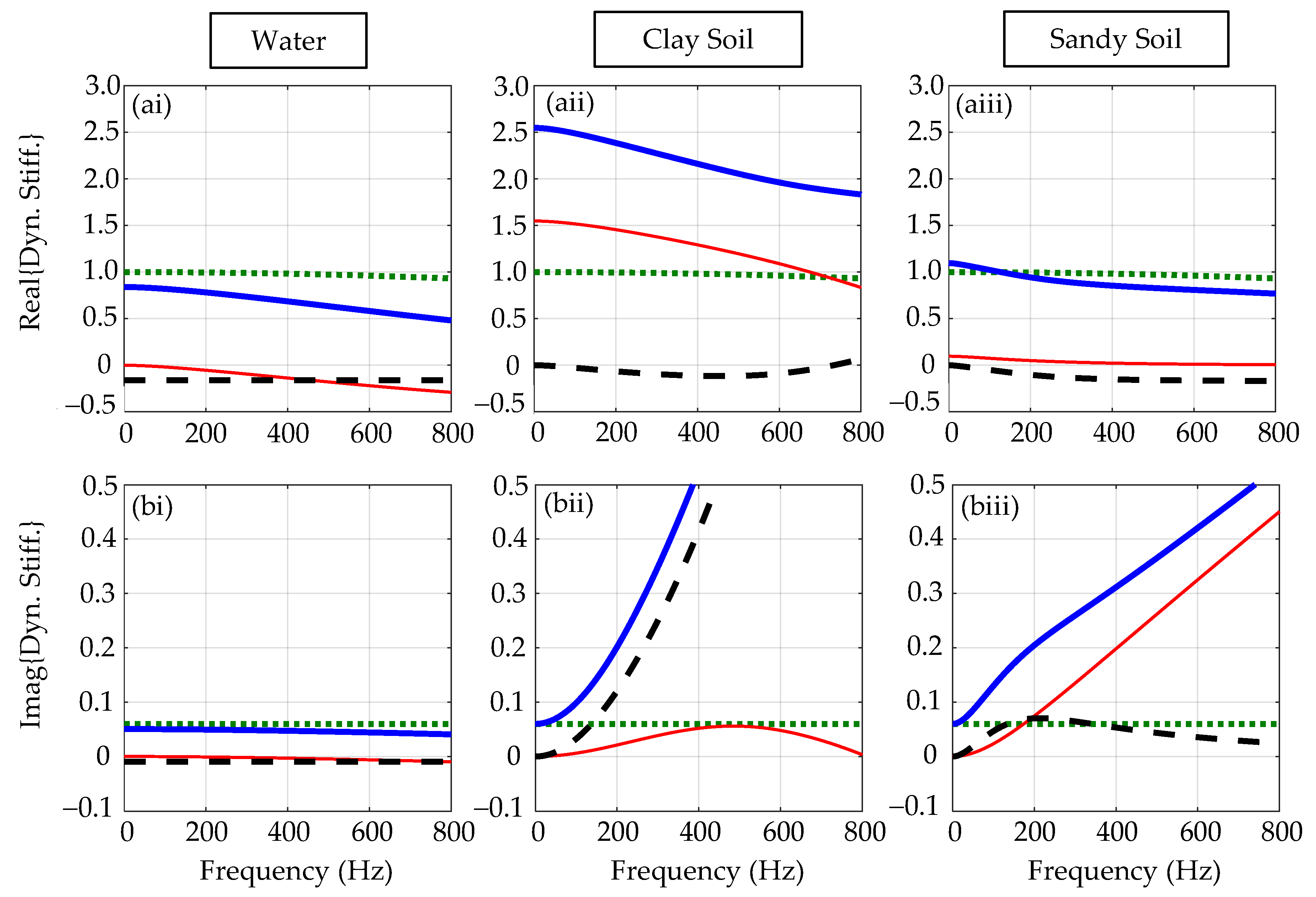
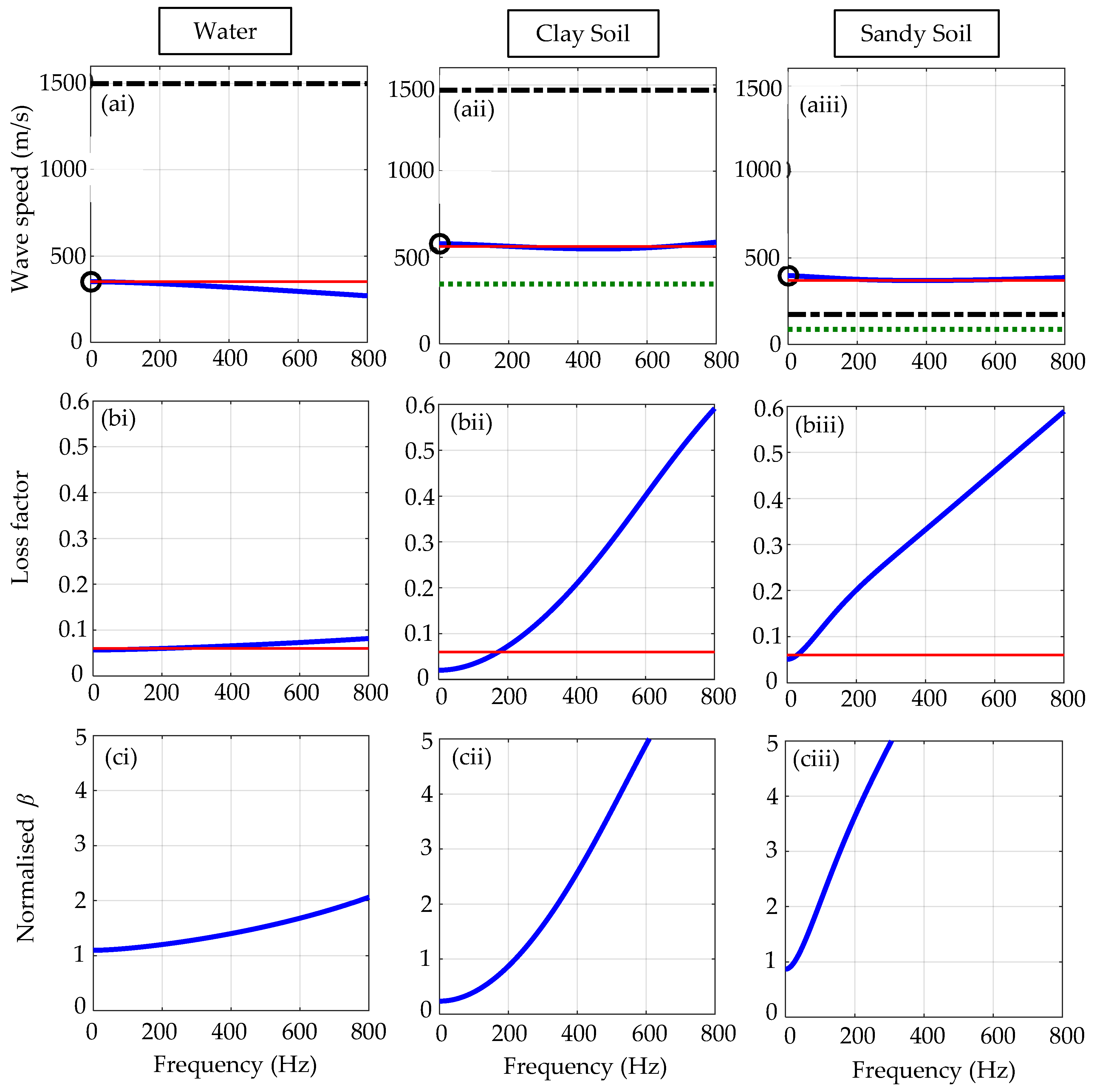
5. Effects of the Component Parts of the System

To illustrate the relative importance of the wave dynamic stiffness terms $K^{(\mathrm{pipe})},$ $K^{(\mathrm{pipe}\text{\_}\mathrm{medium})}$, and $K^{(\mathrm{medium})}$ in Equation (17), their real and imaginary parts are plotted for three conditions in Figure 4a and Figure 4b, respectively. In each case, the pipe is considered to be made from medium-density polyethylene (MDPE), whose dimensions and material properties are given in

Table 3. Medium-density polyethylene (MDPE) pipe properties used in the simulations.

Properties of the MDPE Pipe	Value
Young’s modulus $E_{\mathrm{pipe}}$ (N/m2)	2 × 109
Density ${\rho }_{\mathrm{pipe}}$ (kg/m3)	900
Loss factor ${\eta }_{\mathrm{pipe}}$	0.06
Poisson’s ratio ${\nu }_{\mathrm{pipe}}$	0.4
Pipe mean radius a (mm)	84.5
Pipe wall thickness h (mm)	11

. The properties of three types of surrounding medium, namely water, stiff clay soil, or sandy soil, some of which have been determined from measurements at different test sites, are given in

Table 4. Water and soil properties used in the simulations.

Properties	Water	Stiff Clay Soil	Sandy Soil
Bulk modulus $B_{\mathrm{water}}, B_{\mathrm{medium}}$ (N/m2)	2.25 × 109	4.0 × 109	4.0 × 107
Shear modulus $G_{\mathrm{medium}}$ (N/m2)	0	2.4 × 108	1.5 × 107
Bulk and shear loss factor	0	0	0
Density ${\rho }_{\mathrm{medium}}$ (kg/m3)	1000	2000	2000
Poisson’s ratio	0.5	0.47	0.33
Dilatational wave speed $c_d$ (m/s)	1500	1414	141
Shear wave speed $c_s$ (m/s)	0	346	86

.

If the surrounding medium is water, then no waves radiate from the pipe into the surrounding medium. If the surrounding medium is stiff clay soil, then a shear wave propagates from the pipe into the soil, and if the surrounding medium is sandy soil, then both shear and dilatational waves radiate from the pipe into the soil [20,32].

5.1. Pipe In Vacuo

Before discussing the effects of the different types of surrounding medium, it is instructive to review the in vacuo case with the new formulation, i.e., a water-filled pipe alone, such that $K^{(\mathrm{medium})}=0$. This case has been extensively studied, for example [14,16], so it is only briefly discussed here. Referring to Equation (17), $\mathrm{Re}\left\{K^{\left(\mathrm{pipe}\right)}\right\}=\frac{E_{\mathrm{pipe}}^{ }h}{a^2\left(1-{\nu }_{\mathrm{pipe}}^2\right)}-{\rho }_{\mathrm{pipe}}h{\omega }^2$ and $\mathrm{Re}\left\{K^{(\mathrm{pipe}\text{\_}\mathrm{medium})}\right\}=\frac{-E_{\mathrm{pipe}}^{ }h{\nu }_{\mathrm{pipe}}^2}{a^2\left(1-{\nu }_{\mathrm{pipe}}^2\right)},$ so that $\mathrm{Re}\left\{K^{\left(\mathrm{pipe}\right)}+K^{(\mathrm{pipe}\text{\_}\mathrm{medium})}\right\}=\frac{E_{\mathrm{pipe}}^{ }h}{a^2}-{\rho }_{\mathrm{pipe}}h{\omega }^2,$ which means that the pipe is unconstrained in the axial direction. The term $\frac{E_{\mathrm{pipe}}^{ }h}{a^2}$ is the axially unconstrained hoop stiffness, which is constant with frequency, and the inertial effect of the pipe is given by the term $-{\rho }_{\mathrm{pipe}}h{\omega }^2,$ which is very small for frequencies well below the ring frequency.

For an in vacuo pipe, $\mathrm{Im}\left\{K^{\left(\mathrm{pipe}\right)}\right\}=\frac{E_{\mathrm{pipe}}^{ }h{\eta }_{\mathrm{pipe}}}{a^2\left(1-{\nu }_{\mathrm{pipe}}^2\right)}$ and $\mathrm{Im}\left\{K^{\left(\mathrm{pipe}\text{\_}\mathrm{medium}\right)}\right\}=-\frac{E_{\mathrm{pipe}}^{ }h{\nu }_{\mathrm{pipe}}^2{\eta }_{\mathrm{pipe}}}{a^2\left(1-{\nu }_{\mathrm{pipe}}^2\right)},$ so that $\mathrm{Im}\left\{K^{\left(\mathrm{pipe}\right)}+K^{(\mathrm{pipe}\text{\_}\mathrm{medium})}\right\}=\frac{E_{\mathrm{pipe}}^{ }h{\eta }_{\mathrm{pipe}}^{ }}{a^2},$ which is constant with frequency. Thus, for frequencies well below the ring frequency $K^{(\mathrm{pipe})}+K^{(\mathrm{pipe}\text{\_}\mathrm{medium})}+K^{(\mathrm{medium})}\approx \frac{E_{\mathrm{pipe}}^{ }h}{a^2}\left(1+\mathrm{j}{\eta }_{\mathrm{pipe}}\right).$

5.2. Pipe Surrounded by Water

This case has been studied in [39] and is only briefly discussed here in the context of the new formulation. The real parts of the wave dynamic stiffnesses $K^{(\mathrm{pipe})}, K^{(\mathrm{pipe}\text{\_}\mathrm{medium})} \mathrm{and} K^{(\mathrm{medium})},$ normalised by $\mathrm{Re}\left\{{\tilde{K}}^{\left(\mathrm{pipe}\right)}\right\},$ are plotted in Figure 4(ai) for the case when the pipe is surrounded by water. Note that the model is valid since the upper frequency of 800 Hz is about 1/3 of the ring frequency. The difference between this case and the in vacuo case is that $K^{(\mathrm{medium})}=B_{\mathrm{water}}\frac{k_d^2}{k_d^R}{\overline{H}}_d,$ so that $\mathrm{Re}\left\{K^{(\mathrm{medium})}\right\}=B_{\mathrm{water}}{k}_d^2\mathrm{Re}\left\{\frac{{\overline{H}}_d}{k_d^R}\right\},$ which is negative or equal to zero, and exhibits mass-like behaviour [32]. It can be seen from Figure 4(ai) that $\mathrm{Re}\left\{K^{(\mathrm{medium})}\right\}$ is zero at zero frequency and becomes increasingly negative as frequency increases. Thus, the total real part of the dynamic stiffness, given by the thick solid blue line in Figure 4(ai), has a normalised value corresponding to the axially unconstrained hoop stiffness at zero frequency. It reduces as frequency increases, which is mainly due to the mass loading effect of the surrounding water.

The normalised imaginary parts of the wave dynamic stiffnesses $K^{(\mathrm{pipe})}, K^{(\mathrm{pipe}\text{\_}\mathrm{medium})} \mathrm{and} K^{(\mathrm{medium})}$ are plotted in Figure 4(bi). Again, note that the only difference between this case and the in vacuo case is that $\mathrm{Im}\left\{K^{(\mathrm{medium})}\right\}=B_{\mathrm{water}}{k}_d^2\mathrm{Im}\left\{{\overline{H}}_d/k_d^R\right\},$ which is zero at zero frequency and is small but negative as frequency increases. This means that a small amount of acoustic energy passes from the water to the pipe, which occurs because of decaying wavefields in both the pipe and the soil, with the decay being greater in the pipe than in the soil at any axial position. A normalised dynamic stiffness either higher or lower than the green dotted line means that the component has a greater or lesser effect than that of the pipe.

5.3. Pipe Surrounded by Stiff Clay Soil

The main differences between this case and when the pipe is surrounded by water are that the soil has a shear stiffness and the bulk modulus of the soil is much higher than that of water. In the particular case studied, the shear stiffness of the soil, given by $\frac{2G_{\mathrm{medium}}}{a},$ is larger than the constrained hoop stiffness of the pipe given by $\frac{E_{\mathrm{pipe}}^{ }h}{a^2\left(1-{\nu }_{\mathrm{pipe}}^2\right)}.$ This has an effect on the pipe wave speed and is discussed further in the next section.

The real parts of the wave dynamic stiffnesses $K^{(\mathrm{pipe})}, K^{(\mathrm{pipe}\text{\_}\mathrm{medium})} \mathrm{and} K^{(\mathrm{medium})},$ normalised by $\mathrm{Re}\left\{{\tilde{K}}^{\left(\mathrm{pipe}\right)}\right\},$ are plotted in Figure 4(aii). Note that $\mathrm{Re}\left\{K^{\left(\mathrm{pipe}\right)}\right\}=\frac{E_{\mathrm{pipe}}^{ }h}{a^2\left(1-{\nu }_{\mathrm{pipe}}^2\right)}-{\rho }_{\mathrm{pipe}}h{\omega }^2$ as in the previous case. However, $\mathrm{Re}\left\{K^{(\mathrm{pipe}\text{\_}\mathrm{medium})}\right\}$ is very small in comparison to $\mathrm{Re}\left\{K^{\left(\mathrm{pipe}\right)}\right\},$ and is zero at zero frequency, so that $\mathrm{Re}\left\{K^{\left(\mathrm{pipe}\right)}+K^{(\mathrm{pipe}\text{\_}\mathrm{medium})}\right\}\approx \mathrm{Re}\left\{K^{\left(\mathrm{pipe}\right)}\right\},$ which means that the pipe is constrained in the axial direction due to the shear stiffness of the soil and, consequently, has a higher hoop stiffness than when the pipe is surrounded by water. Note that $\mathrm{Re}\left\{K^{\left(\mathrm{medium}\right)}\right\}$ is about 50% greater than $\mathrm{Re}\left\{K^{\left(\mathrm{pipe}\right)}\right\},$ which can be seen by examining the values at zero frequency in Figure 4(aii). As the wave dynamic stiffness of the soil also exhibits mass-like behaviour, the $\mathrm{Re}\left\{K^{\left(\mathrm{medium}\right)}\right\}$ decreases as frequency increases. Thus, at zero frequency, the total real part of the dynamic stiffness, given by the thick solid blue line in Figure 4(aii), has a normalised value corresponding to the sum of the axially constrained hoop stiffness and the shear stiffness of the soil. It reduces as frequency increases, which is mainly due to the mass loading of the soil.

The normalised imaginary parts of the wave dynamic stiffnesses $K^{(\mathrm{pipe})}, K^{(\mathrm{pipe}\text{\_}\mathrm{medium})} \mathrm{and} K^{(\mathrm{medium})}$ are plotted in Figure 4(bii). Note that $\mathrm{Im}\left\{{\tilde{K}}^{\left(\mathrm{pipe}\right)}\right\}$ is the same as the in vacuo case, and that $\mathrm{Im}\left\{K^{(\mathrm{pipe}\text{\_}\mathrm{medium})}\right\}\gg \mathrm{Im}\left\{K^{(\mathrm{medium})}\right\}$ for frequencies greater than about 200 Hz, so at higher frequencies, $\mathrm{Im}\left\{K^{(\mathrm{pipe}\text{\_}\mathrm{medium})}\right\}$ accounts for the majority of energy dissipation in this case. This means that the axial connection between the pipe and the soil, which was neglected in [32] is an important factor in the leakage of acoustic energy from the pipe to the soil in this case and should be included in a model of the pipe–soil system. At higher frequencies, $\mathrm{Im}\left\{K^{(\mathrm{pipe}\text{\_}\mathrm{medium})}\right\}$ is proportional to frequency, so the energy dissipation due to shear wave propagation in the soil has the effect of adding linear viscous damping to the pipe.

5.4. Pipe Surrounded by Sandy Soil

The main difference between this case and when the pipe is surrounded by clay soil is that the bulk and shear modulus are much smaller. This means that the shear stiffness of the soil only has a marginal effect on the pipe wave speed. However, because both the shear and dilatational wave speed in the soil are smaller than the pipe wave speed, both waves radiate from the pipe, creating a large radiation-damping effect on the pipe.

The real parts of the wave dynamic stiffnesses $K^{(\mathrm{pipe})}, K^{(\mathrm{pipe}\text{\_}\mathrm{medium})} \mathrm{and} K^{(\mathrm{medium})},$ normalised by $\mathrm{Re}\left\{{\tilde{K}}^{\left(\mathrm{pipe}\right)}\right\},$ are plotted in Figure 4(aiii). Note that $\mathrm{Re}\left\{{\tilde{K}}^{\left(\mathrm{pipe}\right)}\right\}$ is the same as in the previous cases. However, $\mathrm{Re}\left\{K^{(\mathrm{pipe}\text{\_}\mathrm{medium})}\right\}$ and $\mathrm{Re}\left\{K^{\left(\mathrm{medium}\right)}\right\}$ are both very small in comparison to $\mathrm{Re}\left\{K^{\left(\mathrm{pipe}\right)}\right\}$, so that $\mathrm{Re}\left\{K^{\left(\mathrm{pipe}\right)}+K^{(\mathrm{pipe}\text{\_}\mathrm{medium})}+K^{(\mathrm{medium})}\right\}\approx \mathrm{Re}\left\{K^{\left(\mathrm{pipe}\right)}\right\},$ which means that although the pipe is constrained in the axial direction due to the shear stiffness of the soil at zero frequency, the surrounding soil only has a marginal stiffening effect at higher frequencies. The slight reduction in the total dynamic stiffness as frequency increases is due to the mass loading effect of the soil as before.

The normalised imaginary parts of the wave dynamic stiffnesses $K^{(\mathrm{pipe})}, K^{(\mathrm{pipe}\text{\_}\mathrm{medium})} \mathrm{and} K^{(\mathrm{medium})}$ are plotted in Figure 4(biii). Note that, as with in the previous cases, $\mathrm{Im}\left\{K^{\left(\mathrm{pipe}\right)}\right\}=\frac{E_{\mathrm{pipe}}^{ }h{\eta }_{\mathrm{pipe}}}{a^2\left(1-{\nu }_{\mathrm{pipe}}^2\right)}$, but for frequencies up to about 100 Hz, $\mathrm{Im}\left\{K^{(\mathrm{pipe}\text{\_}\mathrm{medium})}\right\}\approx \mathrm{Im}\left\{K^{(\mathrm{medium})}\right\}$, and for frequencies greater than about 300 Hz, $\mathrm{Im}\left\{K^{(\mathrm{pipe}\text{\_}\mathrm{medium})}\right\}\ll \mathrm{Im}\left\{K^{(\mathrm{medium})}\right\},$ which is in contrast to the case when the pipe is surrounded by stiff clay soil. At higher frequencies, $\mathrm{Im}\left\{K^{(\mathrm{medium})}\right\}$ is proportional to frequency, so the energy dissipation due to shear and dilatational wave propagation in the soil has the effect of adding linear viscous damping to the pipe.

6. Estimation of Wave Speed and Wave Loss Factor

Approximate expressions for the wave speed and wave loss factor can be determined to gain further physical insight. First, Equation (17), can be written as

$$\frac{k}{k_{\mathrm{water}}}={\left(1+\frac{1}{\mathrm{Re}\left\{\gamma \right\}(1+\mathrm{j}\eta )}\right)}^{\frac{1}{2}}$$

(18)

where $\gamma =\frac{K^{(\mathrm{pipe})}+K^{(\mathrm{pipe}\text{\_}\mathrm{medium})}+K^{(\mathrm{medium})}}{{\tilde{K}}^{(\mathrm{water})}}$ and $\eta =\frac{\mathrm{Im}\left\{\gamma \right\}}{\mathrm{Re}\left\{\gamma \right\}}$ is the combined loss factor for the pipe wall, the surrounding medium, and the water contained in the pipe. If $\eta \ll 1,$ then Equation (18) can be written as

$$\frac{k}{k_{\mathrm{water}}}={\left(1+\frac{1}{\mathrm{Re}\left\{\gamma \right\}}\right)}^{\frac{1}{2}}{\left(1-\frac{\mathrm{j}\eta }{2\left(1+\mathrm{Re}\left\{\gamma \right\}\right)}\right)}^{\frac{1}{2}}$$

(19)

Noting that $c=\frac{\omega }{\mathrm{Re}\left\{k\right\}}$ and ${\eta }_{\mathrm{wave}}=-\frac{2\mathrm{Im}\left\{k\right\}}{\mathrm{Re}\left\{k\right\}},$ the wave speed and loss factor associated with this wave for a small loss factor are given by

$$c\approx c_{\mathrm{water}}{\left(1+\frac{1}{\mathrm{Re}\left\{\gamma \right\}}\right)}^{-\frac{1}{2}}$$

(20a)

$${\eta }_{\mathrm{wave}}\approx \frac{\eta }{1+\mathrm{Re}\left\{\gamma \right\}}$$

(20b)

The wave speeds and wave loss factors for the pipe systems surrounded by the three surrounding media whose parameters are given in Table 4 are shown in Figure 5a and Figure 5b, respectively. Figure 5c shows $\beta =\frac{{\eta }_{\mathrm{wave}}}{2c}$ normalised by the attenuation factor for a massless in vacuo pipe.

6.1. Pipe In Vacuo

This is the benchmark case which the others are compared with. As the loss factor of the pipe wall is much less than one, the wave speed is given by Equation (20a). If the mass of the pipe is neglected, then $\mathrm{Re}\left\{\gamma \right\}=\frac{E_{\mathrm{pipe}}h/a^2}{2B_{\mathrm{water}}a},$ which is the ratio of the axially unconstrained hoop stiffness of the pipe and the stiffness of the water inside the pipe. For the parameters given in Table 3 and Table 4, $\mathrm{Re}\left\{\gamma \right\}\approx 0.06,$ which results in a wave speed of about 351 m/s. This reduces marginally with frequency due to the mass of the pipe wall. The wave loss factor is given with Equation (20b) which, for the parameters given in Table 3 and Table 4, is given by ${\eta }_{\mathrm{wave}}\gg {\eta }_{\mathrm{pipe}},$ and is constant with frequency. If the mass of the pipe wall is neglected, the loss factor of the pipe is much less than unity, and $\mathrm{Re}\left\{\gamma \right\}\ll 1,$ which is the case for the pipe with the parameters given in Table 1, then $\beta \approx \frac{{\eta }_{\mathrm{pipe}}}{2c_{\mathrm{water}}{\left(\mathrm{Re}\left\{\gamma \right\}\right)}^{\frac{1}{2}}}=3.5\times {10}^{-4}$ s/m. Note that this term is constant with frequency.

6.2. Pipe Surrounded by Water

The wave speed is plotted in Figure 5(ai). Also plotted in this figure is the wave speed for a massless in vacuo pipe for comparison, and the wave speed of the dilatational wave in the surrounding water. The main effect of the mass of the pipe and the mass-loading effect of the surrounding water is to marginally reduce the wave speed as frequency increases from $c\approx c_{\mathrm{water}}{\left(1+\frac{2B_{\mathrm{water}}a}{E_{\mathrm{pipe}}h/a^2}\right)}^{-\frac{1}{2}}$ at zero frequency, which is shown as the circle in Figure 5(ai). The wave loss factor is plotted in Figure 5(bi) together with the loss factor of the pipe. It can be seen that at zero frequency, ${\eta }_{\mathrm{wave}}\approx {\eta }_{\mathrm{pipe}},$ as the added mass effect has no influence at this frequency. It can also be seen that the loss factor marginally increases with frequency, which is because $\mathrm{Re}\left\{k\right\}$ reduces because of the mass loading of the surrounding water. Note that because no waves propagate from the pipe into the water, the acoustic energy is constrained in the pipe.

Combining the wave speed and the wave loss factor gives the attenuation factor $\beta .$ This is normalised by the attenuation factor for the massless in vacuo case discussed in Section 5.1 and is plotted in Figure 5(ci). It can be seen that this increases with frequency, which is due to a small increase in the wave loss factor and a larger decrease in the wave speed. Both are predominantly due to the mass loading of the surrounding water.

6.3. Pipe Surrounded by Stiff Clay Soil

The wave speed is plotted in Figure 5(aii), together with the shear and dilatational wave speeds in the soil. As there is significant loss in the system at higher frequencies, Equation (20a) is only valid at low frequencies (less than about 100 Hz). At zero frequency, however, Equation (20a) is valid and $\mathrm{Re}\left\{\gamma \left(0\right)\right\}=\left(\frac{E_{\mathrm{pipe}}h{\eta }_{\mathrm{pipe}}}{a^2\left(1-{\nu }_{\mathrm{pipe}}^2\right)}+\frac{2G_{\mathrm{medium}}}{a}\right)/\left(\frac{2B_{\mathrm{water}}}{a}\right).$ For the parameters given in Table 3 and Table 4, $\mathrm{Re}\left\{\gamma \left(0\right)\right\}=0.18,$ which gives a wave speed of approximately 585 m/s. This is shown as the circle in Figure 5(aii). It can be seen that as frequency increases, the wave speed first decreases by a small amount, which is due predominantly to the mass loading of the soil, and then increases by a small amount, which is due to the shear wave radiation into the soil. Note that the dilatational wave does not propagate away from the pipe because the dilatational wave speed is greater than the wave speed in the pipe. However, because the shear wave speed in the soil is non-zero but smaller than the pipe wave speed, it propagates at an angle of approximately 59° from the axis of pipe, leaking energy into the soil.

The wave loss factor is plotted in Figure 5(bii) together with the loss factor of the pipe. It can be seen that at low frequencies, below about 200 Hz, the wave loss factor is significantly less than the pipe loss factor. At zero frequency, it is given by ${\eta }_{\mathrm{wave}}\approx \frac{{\eta }_{\mathrm{pipe}}}{1+\mathrm{Re}\left(\gamma \left(0\right)\right)}.$ It is clear that the large shear stiffness of the soil is responsible for this. As the frequency increases, the wave loss factor increases significantly, and this is due to the leakage of energy from the pipe into the soil, by way of the radiated shear wave. The normalised value of $\beta$ is plotted in Figure 5(cii). It can be seen that this is less than unity at zero frequency, but it increases rapidly with frequency. Concerning the two factors that affect this parameter, the pipe wave speed is approximately constant with frequency, so the wave loss factor is the main influence on the frequency dependency of $\beta .$

6.4. Pipe Surrounded by Sandy Soil

The wave speed is plotted in Figure 5(aiii), together with the shear and dilatational wave speeds in the soil. As with the clay soil, there is a significant loss in the system at higher frequencies, so Equation (20a) is only valid at low frequencies (less than about 100 Hz). At zero frequency, $\mathrm{Re}\left\{\gamma \left(0\right)\right\}=\left(\frac{E_{\mathrm{pipe}}h{\eta }_{\mathrm{pipe}}}{a^2\left(1-{\nu }_{\mathrm{pipe}}^2\right)}+\frac{2G_{\mathrm{medium}}}{a}\right)/\left(\frac{2B_{\mathrm{water}}}{a}\right),$ and for the parameters in Table 3 and Table 4, $\mathrm{Re}\left\{\gamma \left(0\right)\right\}=0.08$. This results in a wave speed of about 398 m/s, which remains roughly constant over the whole frequency range shown. Because the shear and dilatational wave speeds in the soil are smaller than the pipe wave speed, they propagate at angles of approximately 77° and 66°, respectively, from the axis of pipe, leaking energy into the soil.

The wave loss factor is plotted in Figure 5(biii) together with the loss factor of the pipe. It can be seen that for practically the whole frequency range, the wave loss factor is greater than the pipe loss factor. At zero frequency, it is given by ${\eta }_{\mathrm{wave}}\approx {\eta }_{\mathrm{pipe}},$ and then increases almost linearly with frequency. At low frequencies, the loss is significantly greater than that for the clay soil which is due to two things: The first is that the soil does not have a significant stiffening effect, and the second is that two waves, rather than one, propagate energy from the pipe into the soil. The normalised value of $\beta$ is plotted in Figure 5(ciii). Because the pipe wave speed is approximately constant with frequency, the dominant influence on this parameter is the wave loss factor.

7. Conclusions

This paper has presented a detailed investigation into the physical mechanisms of leak noise propagation in buried plastic water pipes, which include the material properties of the system, the geometry, and, importantly, the interface between the pipe and soil. To facilitate this work, an alternative physics-based model for the wavenumber of a buried plastic water pipe was developed. By assuming that there is only one dominant wave in the pipe, namely the predominantly fluid-borne wave, a compact model of the wavenumber has been presented. This involves the wave dynamic stiffness matrices of the component parts of the system. It has been shown that, although the shear stiffness of the soil and the hoop stiffness of the pipe have a strong influence on the wave speed, the axial connection between the pipe and the soil can have a significant impact on wave attenuation in some situations. To support the theoretical modelling, some experiments were performed on two test rigs characterised by distinct pipe and soil properties. The model gave good predictions of the experimental results in both cases. The new model can, therefore, predict the wave behavior in buried plastic water pipes, and hence be used to determine the factors governing the way in which leak noise propagates in them.

References

1. Mohd Yussof, N.A.; Ho, H.W. Review of Water Leak Detection Methods in Smart Building Applications. Buildings 2022, 12, 1535. [Google Scholar] [CrossRef]
2. El-Zahab, S.; Zayed, T. Leak detection in water distribution networks: An introductory overview. Smart Water 2019, 4, 5. [Google Scholar] [CrossRef]
3. Puust, R.; Kapelan, Z.; Savic, D.A.; Koppel, T. A review of methods for leakage management in pipe networks. Urban Water J. 2010, 7, 25–45. [Google Scholar] [CrossRef]
4. Romero-Ben, L.; Alves, D.; Blesa, J.; Cembrano, G.; Puig, V.; Duviella, E. Leak detection and localization in water distribution networks: Review and perspective. Annu. Rev. Control. 2023, 55, 392–419. [Google Scholar] [CrossRef]
5. Hu, Z.; Tariq, S.; Zayed, T. A comprehensive review of acoustic based leak localization method in pressurized pipelines. Mech. Syst. Sig. Process. 2021, 161, 107994. [Google Scholar] [CrossRef]
6. Kanakoudis, V.; Muhammetoglu, H. Urban Water Pipe Networks Management Towards Non-Revenue Water Reduction: Two Case Studies from Greece and Turkey. Clean Soil Air Water 2014, 42, 880–892. [Google Scholar] [CrossRef]
7. Chew, A.W.Z.; Kalfarisi, R.; Meng, X.; Pok, J.; Wu, Z.Y.; Cai, J. Acoustic feature-based leakage event detection in near real-time for large-scale water distribution networks. J. Hydroinform. 2023, 25, 526–551. [Google Scholar] [CrossRef]
8. EEA Report, Use of Freshwater Resources in Europe. 2019. Available online: https://www.eea.europa.eu/en/analysis/indicators/use-of-freshwater-resources-in-europe-1 (accessed on 14 December 2023).
9. EurEau Report, Europe’s Water in Figures. 2017. Available online: https://www.eureau.org/resources/publications/eureaupublications/5824-europe-s-water-in-figures-2021/file (accessed on 14 December 2023).
10. Globo Report. 2019. Available online: https://g1.globo.com/economia/noticia/2019/06/05/oito-estados-do-pais-perdem-metade-ou-mais-da-agua-que-produzem-com-vazamentos-e-gatos-diz-estudo.ghtml (accessed on 14 December 2023).
11. Hunaidi, O.; Chu, W.T. Acoustic characteristics of leak signals in water distribution pipes. Appl. Acoust. 1999, 58, 235–254. [Google Scholar] [CrossRef]
12. Fan, H.; Tariq, S.; Zayed, T. Acoustic leak detection approaches for water pipelines. Autom. Constr. 2022, 138, 104226. [Google Scholar] [CrossRef]
13. Keramat, A.; Ahmadianfar, I.; Duan, H.F.; Hou, Q. Spectral transient-based multiple leakage identification in water pipelines: An efficient hybrid gradient-metaheuristic optimization. Expert Syst. Appl. 2023, 224, 120021. [Google Scholar] [CrossRef]
14. Pinnington, R.J.; Briscoe, A.R. Externally applied sensor for axisymmetric waves in a fluid filled pipe. J. Sound Vib. 1994, 173, 503–516. [Google Scholar] [CrossRef]
15. Pinnington, R.J. The axisymmetric wave transmission properties of pressurized flexible tubes. J. Sound Vib. 1997, 204, 271–289. [Google Scholar] [CrossRef]
16. Muggleton, J.M.; Brennan, M.J.; Linford, P.W. Axisymmetric wave propagation in fluid-filled pipes: Wavenumber measurements in in vacuo and buried pipes. J. Sound Vib. 2004, 270, 171–190. [Google Scholar] [CrossRef]
17. Available online: https://www.youtube.com/watch?v=81RxkjhBv5s&t=1158s (accessed on 13 December 2023).
18. Kafle, D.M.; Fong, S.; Narasimhan, S. Active acoustic leak detection and localization in a plastic pipe using time delay estimation. Appl. Acoust. 2022, 187, 108482. [Google Scholar] [CrossRef]
19. Santoni, A.; Marzola, I.; Alvisi, S.; Fausti, P.; Stefanelli, C. Influence of noise masking on leak pinpointing: Experimental analysis on a laboratory test rig for leak noise correlation. Appl. Acoust. 2023, 214, 109710. [Google Scholar] [CrossRef]
20. Scussel, O.; Brennan, M.J.; Almeida, F.C.L.; Iwanaga, M.K.; Muggleton, J.M.; Joseph, P.F.; Gao, Y. Key Factors That Influence the Frequency Range of Measured Leak Noise in Buried Plastic Water Pipes: Theory and Experiment. Acoustics 2023, 5, 490–508. [Google Scholar] [CrossRef]
21. Fuller, C.; Fahy, F.J. Characteristics of wave propagation and energy distributions in cylindrical elastic shells filled with fluid. J. Sound Vib. 1982, 81, 501–518. [Google Scholar] [CrossRef]
22. Xu, M.; Zhang, W. Vibrational power flow input and transmission in a circular cylindrical shell filled with fluid. J. Sound Vib. 2000, 234, 387–403. [Google Scholar] [CrossRef]
23. Sinha, B.K.; Plona, T.J.; Kostek, S.; Chang, S.K. Axisymmetric wave propagation in fluid loaded cylindrical shells. I: Theory. J. Acoust. Soc. Am. 1992, 92, 1132–1143. [Google Scholar] [CrossRef]
24. Pan, H.; Koyano, K.; Usui, Y. Experimental and numerical investigations of axisymmetric wave propagation in cylindrical pipe filled with fluid. J. Acoust. Soc. Am. 2003, 113, 3209–3214. [Google Scholar] [CrossRef]
25. Prek, M. Analysis of wave propagation in fluid-filled viscoelastic pipes. Mech. Syst. Sig. Process. 2007, 21, 1907–1916. [Google Scholar] [CrossRef]
26. Long, R.; Cawley, P.; Lowe, M. Acoustic wave propagation in buried iron water pipes. Proc. R. Soc. Lond. Ser. A Math. Phys. Eng. Sci. 2003, 459, 2749–2770. [Google Scholar] [CrossRef]
27. Long, R.; Lowe, M.; Cawley, P. Attenuation characteristics of the fundamental modes that propagate in buried iron water pipes. Ultrasonics 2003, 41, 509–519. [Google Scholar] [CrossRef]
28. Deng, Q.T.; Yang, Z.C. Wave propagation analysis in buried pipe conveying fluid. Appl. Math. Model. 2013, 37, 6225–6233. [Google Scholar] [CrossRef]
29. Leinov, E.; Lowe, M.J.; Cawley, P. Investigation of guided wave propagation and attenuation in pipe buried in sand. J. Sound Vib. 2015, 347, 96–114. [Google Scholar] [CrossRef]
30. Muggleton, J.M.; Yan, J. Wavenumber prediction and measurement of axisymmetric waves in buried fluid-filled pipes: Inclusion of shear coupling at a lubricated pipe/soil interface. J. Sound Vib. 2013, 332, 1216–1230. [Google Scholar] [CrossRef]
31. Yan, J.; Zhang, J. Characteristics of vibrational wave propagation and attenuation in submarine fluid-filled pipelines. China Ocean Eng. 2015, 29, 253–263. [Google Scholar] [CrossRef]
32. Brennan, M.J.; Karimi, M.; Muggleton, J.M.; Almeida, F.C.L.; de Lima, F.K.; Ayala, P.C.; Obata, D.; Paschoalini, A.T.; Kessissoglou, N. On the effects of soil properties on leak noise propagation in plastic water distribution pipes. J. Sound Vib. 2018, 427, 120–133. [Google Scholar] [CrossRef]
33. Gao, Y.; Sui, F.; Muggleton, J.M.; Yang, J. Simplified dispersion relationships for fluid-dominated axisymmetric wave motion in buried fluid-filled pipes. J. Sound Vib. 2016, 375, 386–402. [Google Scholar] [CrossRef]
34. Liu, Y.; Habibi, D.; Chai, D.; Wang, X.; Chen, H. A Numerical Study of Axisymmetric Wave Propagation in Buried Fluid-Filled Pipes for Optimizing the Vibro-Acoustic Technique When Locating Gas Pipelines. Energies 2019, 12, 3707. [Google Scholar] [CrossRef]
35. Wang, Y.Q.; Cao, D.Y.; Zhang, Y.F. Wave Propagation for Axisymmetric Wave Motion in Buried Pipes Conveying Viscous Flowing Fluid. J. Pipeline Syst. Eng. Pract. 2021, 12, 04021044. [Google Scholar] [CrossRef]
36. Fahy, F.; Gardonio, P. Sound and Structural Vibration: Radiation, Transmission and Response, 2nd ed.; Elsevier: Oxford, UK, 2007. [Google Scholar]
37. Nashif, A.D.; Jones, D.I.G.; Henderson, J.P. Vibration Damping, 1st ed.; Wiley: Hoboken, NJ, USA, 1985. [Google Scholar]
38. Ewing, W.M.; Jardetzky, W.S.; Press, F.; Beiser, A. Elastic Waves in Layered Media; McGraw-Hill: New York, NY, USA, 1957. [Google Scholar]
39. Muggleton, J.M.; Brennan, M.J. Leak noise propagation and attenuation in submerged plastic water pipes. J. Sound Vib. 2004, 278, 527–537. [Google Scholar] [CrossRef]
Figure 1. A schematic diagram of a water-filled buried pipe (a) general layout; (b) applied forces and coordinate system.
Acoustics 06 00009 g001
Figure 2. Photographs and schematic diagrams of the test rigs (not to scale): (a) São Paulo, Brazil (clay soil) and (b) Blithfield, UK (sandy soil).
Acoustics 06 00009 g002
Figure 3. Comparison of measurements made on the two sites shown in Figure 2 and predictions made using the model with the parameters given in Table 1 and Table 2. (a) São Paulo, Brazil (clay soil); (b) Blithfield, UK (sandy soil). (i) wave speed, (ii) attenuation, (iii) coherence (thick blue solid lines); predictions (thin black solid lines). The shaded region bounded by the red thick dotted lines denotes the bandwidth where there is good coherence.
Acoustics 06 00009 g003
Figure 4. Normalised real (a) and imaginary parts (b) of the wave dynamic stiffness in Equation (17) for three systems with the same buried MDPE pipe for a surrounding medium of (i) water, (ii) clay soil, and (iii) sandy soil; K ( pipe ) / Re K ˜ ( pipe ) (green dotted line); K ( pipe _ soil ) / Re K ˜ ( pipe ) (black dashed line); K ( soil ) / Re K ˜ ( pipe ) (thin red solid line); K ( pipe ) + K ( pipe _ soil ) + K ( soil ) / Re K ˜ ( pipe ) (thick solid blue line).
Acoustics 06 00009 g004
Figure 5. Properties of the three systems corresponding to those in Figure 4 for a surrounding medium of (i) water, (ii) clay soil, and (iii) sandy soil; (a) Wave speeds; massless in vacuo pipe (thin red solid line); pipe surrounded by the medium, (thick blue solid line); shear wave in the external medium (thick green dotted line); dilatational wave in the external medium (thick black dashed-dotted line). (b) Loss factors; pipe surrounded by external medium (thick blue solid line); massless in vacuo pipe (thin red solid line). (c) Normalised value of β .
Acoustics 06 00009 g005