1. Introduction
Active vibration control in rotors has been a well-known field of research during the last five decades. Due to the uncertainty of external disturbances, robust controllers seem to be suitable candidates for vibration suppression in rotors. However, the research on this subject, particularly for rotor vibration, is limited.
Early investigations considering
H∞ control for short rotors showed the existence of a controller in the frequency domain [
1,
2]. They have been used to control vibrations via Active Magnetic Bearings (AMBs). The experimental verification of such robust controllers has been conducted [
3], and recently, effectiveness of the controllers for short rotors has been demonstrated [
4].
Apart from experimental attempts, a theoretical investigation of optimal controllers and robust-type vibration suppressors via AMBs has been performed for short rotors that are assumed rigid [
5,
6]. For short and flexible rotors, optimal controllers have also been studied [
7]. However, the multivariable model requirement for rotor vibration control (even for rigid short rotors) is studied and demonstrated in [
8].
For the vibration control of flexible and long rotors, an experimental and theoretical analysis is carried out in [
9], and the multivariable nature of controllers is emphasized in [
10]. Moreover, it has been shown that there exist controllers that suppress vibrations at resonance [
11].
Recently vibration suppression in long flexible rotors was studied, in which the existence of realizable controllers subject to any kind of disturbance was investigated and commented upon [
12]. However, the comparative performance of robust vibration controllers in both the time and frequency domain for long and flexible rotors has not been carried out yet.
In this paper, the long flexible rotor system that is described in [
12] is considered for investigation. The
H∞ optimality criteria was selected for the purposes of comparison. Therefore, the
H∞ control problem is initially formulated. Thereafter, a mixed-sensitivity
H∞ criterion, which is an appropriate method for the investigation of disturbance rejection in vibration control problems, is described.
An iterative algorithm is introduced, enabling robust controllers, which can also be H∞ optimal, to be determined. It is shown that for the rotor system model, the resulting controller can be realizable with a low order. However, satisfying the H∞ optimality condition does not guarantee an appropriate system response when operating under severe disturbances.
Moreover, via a singular value analysis, it is concluded that the singular values for the sensitivity matrix are not the only factors to be considered for performance evaluation. Further reduction in the H∞ norm for the KS matrix is required to decrease the control effort and avoid high amplitude oscillations. Finally, an appropriate system response is achievable, but it requires a high-order multivariable controller. The transfer function matrix of such a controller in the frequency domain and its complexity and feasibility are discussed and commented upon.
2. Open-Loop Transfer Function Matrix Estimation
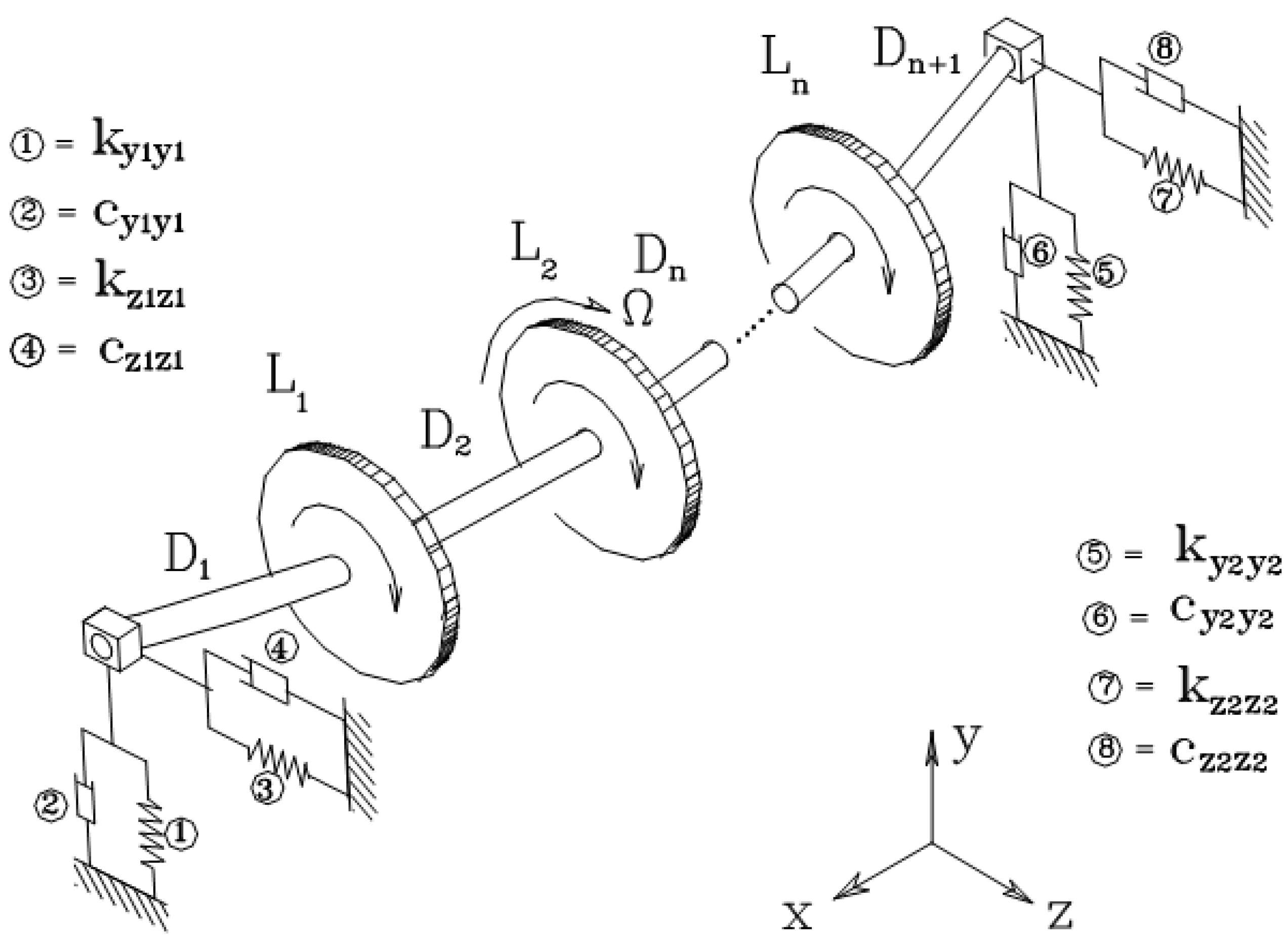
A rotor can be idealized as
n + 1 of the distributed parameter shafts. Those shafts are connected via
n lumped parameter disks. The overall assembly is mounted on bearings and is shown in
Figure 1.
The vibration of the mth lumped disk in the vertical y direction, which results from the vertical excitation force at the lth lumped element, can be computed using the flexibility matrix as follows:
The vibration of the
mth lumped disk in the vertical
y direction, which results from the vertical excitation force at the
lth lumped element, can be computed using the flexibility matrix as follows:
where
in (1) is the frequency response function, in which the corresponding flexibility matrix is as follows:
The matrices
K in the flexibility matrix are defined by the following:
where the
T matrices in (2) are as follows:
The parameter with and where A is the cross-sectional area, E is the modulus of elasticity, and I is the moment of inertia of the cross section in bending.
The matrices
D in (1) are defined by the following:
Jp and Jt are the polar and transverse moments of inertia of the lumped disc. In the above equations, s is the Laplace variable, m is the mass of each lumped element, Ω is the rotational speed of the shaft, and ρ is the density of the shaft material. L is the length of each distributed element.
The matrices
B are defined by the following:
The above partitioned flexibility matrix is described in [
12] based on the dynamic stiffness matrix method (DSMM), in which each of the sub-matrices is described in [
12].
Frequency response data can be obtained from each transfer function, so that a vector of the frequency response data, as a function of
, could be written as follows.
xpq and
ypq in (3) and (4) are the real and imaginary parts of the transfer function
G’.
From the multivariable frequency response matrix in Equations (3) and (4), estimates of the transfer functions can be obtained in the following form [
12]:
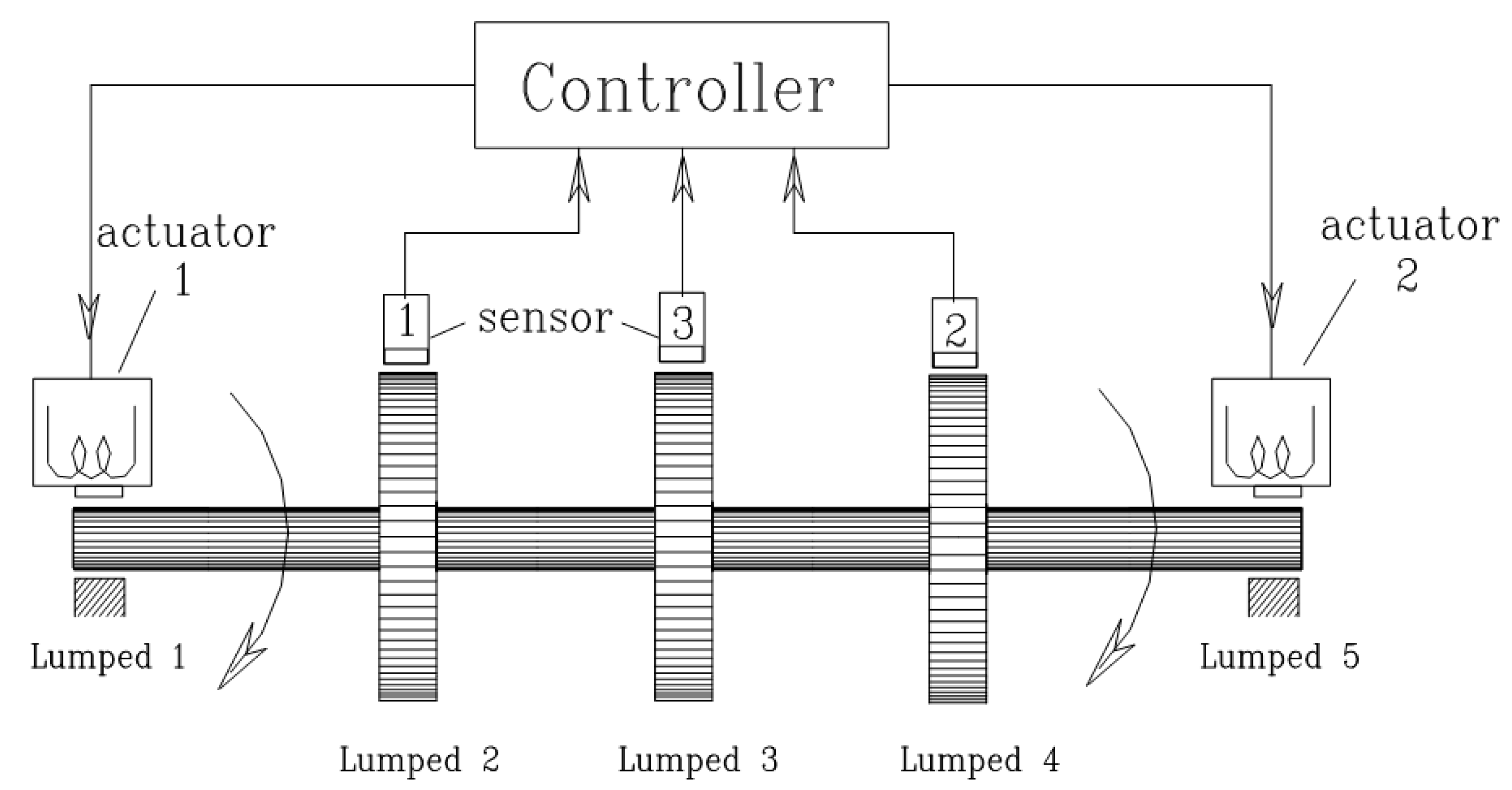
The schematic diagram of the closed-loop vibration control system for the rotor system is shown in
Figure 2:
In the above open-loop system, the transfer function matrix is as follows:
In (6), and are the transformed functions of the measured vibration amplitude via sensors 1 and 2, and and are the transformed functions of control forces applied via the actuators 1 and 2.
The individual transfer functions in (6) were estimated via [
12]
and
The input control effort vector is
, and the measurement variable vector is
. The controller designated by the matrix
should be designed to apply the control force
to the rotor system
G(
s) via the actuators. In the terminology of robust control that will be described in
Section 4, the
G(
s) is a part of the plant that is designated by the matrix
.
3. Formulation of the H∞ Control Problem
In the early eighties, investigations aimed at reducing closed-loop control system sensitivity were undertaken. Initially, a sensitivity reduction analysis for MIMO systems was formulated by Zames [
13] as an optimisation problem. He employed a functional analysis and used transformations, matrix norms, and approximate inverses in his procedures.
Thereafter, this area of research was developed by introducing the robust control theory and
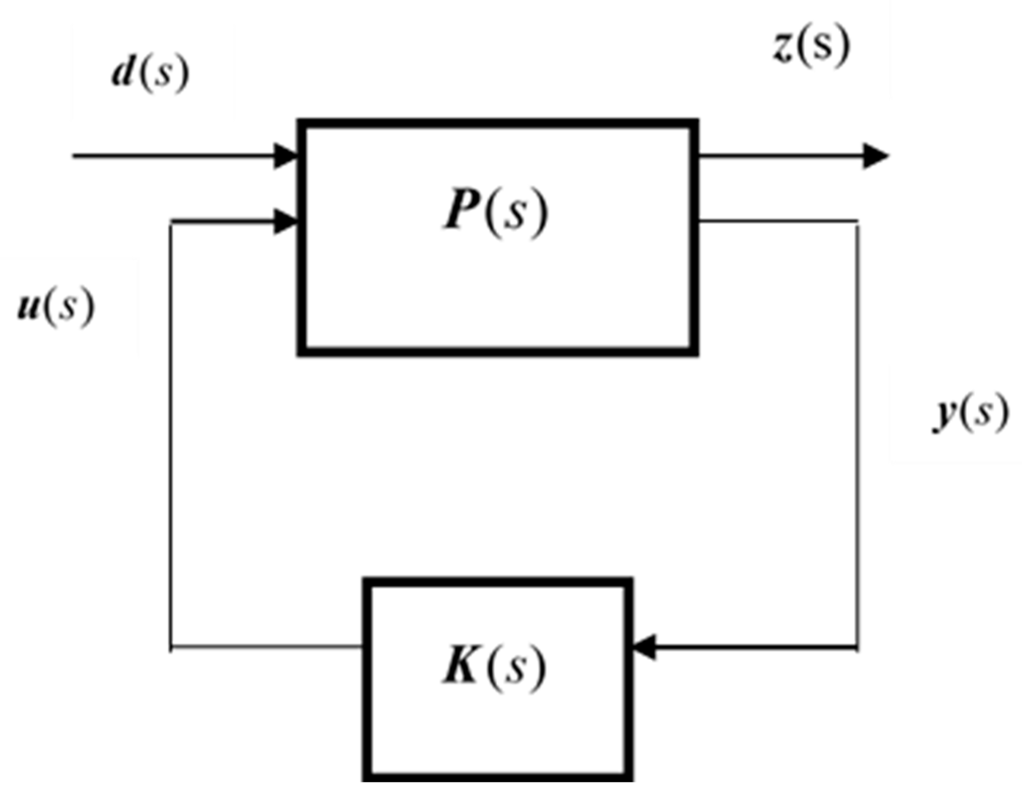
H∞ optimal control to design controllers. By defining new transformations, further algorithms were developed, simplifying the design procedures. General control configurations can be investigated by
H∞ methods, described by the block diagram in
Figure 3:
The input disturbance vector is denoted by
, the output error and control signal vector is
, the input control effort vector is
, and the measurement variable vector is
. The controller model is designated by the matrix
and the plant by the matrix
. This general control configuration can be expressed by the following:
The plant
consists of four sub-matrices, which satisfy the following relations:
The controller applies the control effort based on the measured variables, such that
Upon eliminating
u and
y from Equations (12)–(14), the following relationship is obtained:
where
In Equations (15) and (16),
is known as the lower Linear Fractional Transformation (LFT), described by Glover [
14], which determines the system output
z, following disturbances.
A sensible representation for the disturbance vector
can be obtained by using the second norm of the signal
d(
t) as follows (see, for example, Desoer and Vidyasagar [
15]):
where
n is number of inputs and outputs. Similarly, for the output vector
, the second norm of
z(
t) would be as follows:
where 2
n is used when there are two output channels, and where, in some cases, there may be more than 2
n outputs. However, the question of interest is “If we know how large the input disturbances are, how large are the outputs going to be ?” Doyle et al. [
16].
The answer is that an upper bound for the output can be determined. This upper bound can be expressed by using the
H∞ norm via the following relationship:
where the symbol
is used for the
H∞ norm, which can be computed from the following:
The symbol
indicates the maximum singular value of the matrix
at each frequency
ω, remembering that (17) and (18) are valid for any two signals, which can be related by a transfer function matrix. The proof for SISO systems is given in Doyle et al. [
16] and for MIMO systems in Zhou et al. [
17]. Therefore, the
H∞ control problem can be summarised by the following statement from Skogestad et al. [
18].
Find all stabilising controllers
K, such that
γ in (21) is a parameter that is chosen via weighting functions.
4. Mixed-Sensitivity H∞ Control
This form of a control strategy was employed for disturbance rejection purposes by Yue and Postlethwaite [
19] for a helicopter control system. The minimum effort control method herein, which can be converted into a mixed-sensitivity
H∞ form, enabling
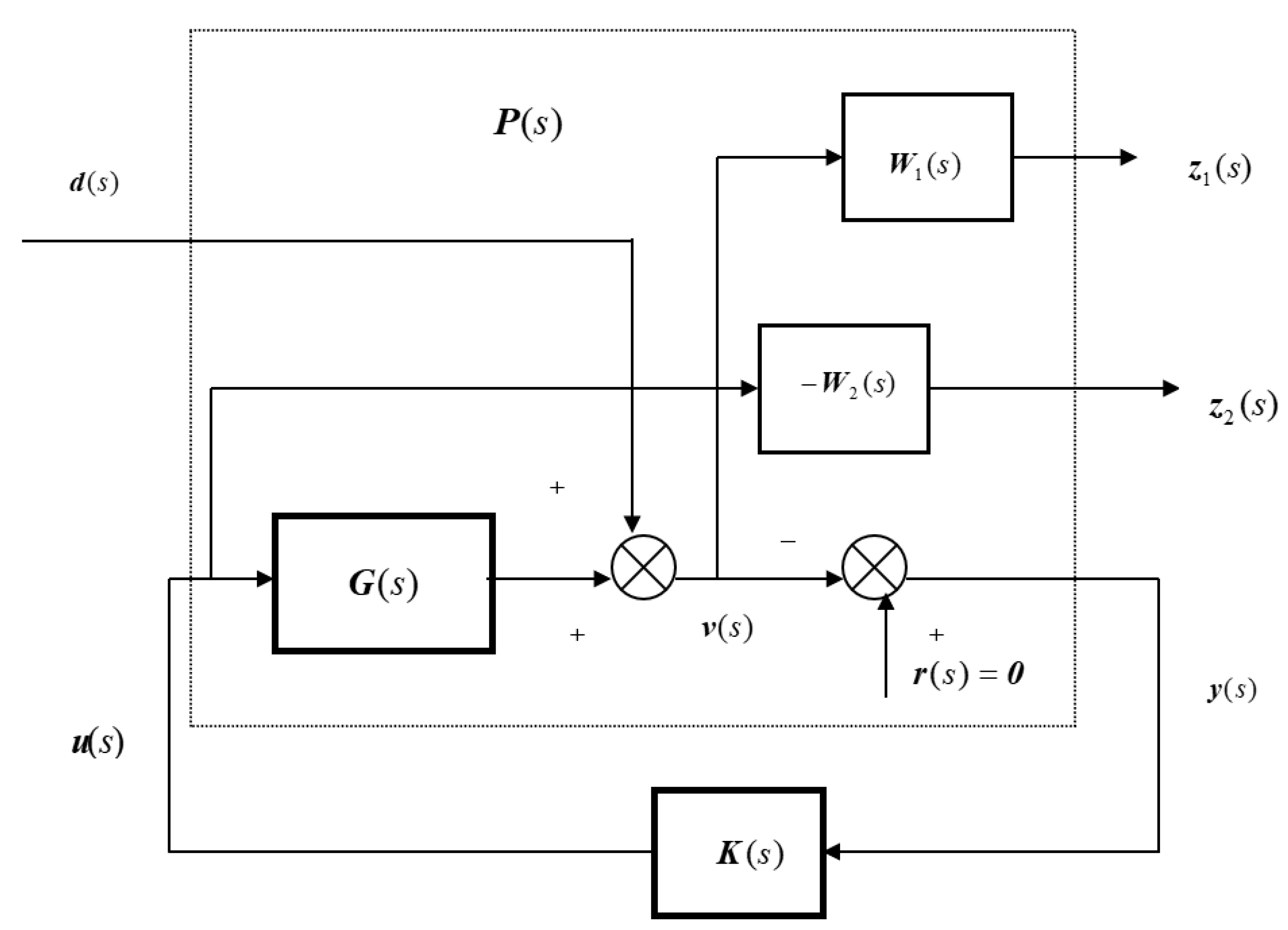
H∞ optimality, is to be confirmed. The control system configuration is shown in
Figure 4, describing how disturbance rejection can be achieved.
The output Is a combination of
, which is the weighted error of the system, and
, which is the weighted control effort, where
Because the set point vector is null, the error vector
and measured variable vector
are equal, with opposite signs. The
z vector can be computed from the following:
By defining the sensitivity matrix of the system as follows:
It can be shown that (23) and (24) may be rewritten as follows:
Then the sub-matrices of the plant
can be computed from the following relations
O is empty matrix:
The partitioned matrix relationship is as follows:
Upon the substitution of (28) into (16), if the LFT of the system can be computed as
then relation (19) in this case would be as follows:
Therefore, if a stabilising controller
K is selected for the system which satisfies the relation
then the output of the system
z is bounded by following inequality:
It is common practice to select the appropriate weighting matrices
W1 and
W2 for the error and control effort vectors. These matrices are diagonal as follows:
The shape of
in (34)–(35) depends on the frequency range of interest. In Skogestad et al. [
18],
functions are recommended for process control applications. The weighting function
for the control effort can usually be formulated in order to achieve an appropriate minimum.
Moreover, both the low and high frequency singular value characteristics are of interest in machine vibration problems. The singular values of the sensitivity matrix at low frequencies are required for the assessment of step-response transients, while the high frequency values give information on noise attenuation. However, for a significant disturbance rejection at a steady state, the sensitivity weighting function could be represented by the following:
The weighting function
should have small gains at a low frequency, bounding the sensitivity matrix so that
The forms in (37) and (36) are also recommended by Postlethwaite in [
19]. In order to achieve a lower control effort,
should approach unity. The functions
and
represent upper bounds for the sensitivity and control effort, respectively.
Similarly, both the upper and lower bounds of the sensitivity matrix should be considered to evaluate the effectiveness of the controller. This requires the determination of the maximum and minimum singular values of the sensitivity matrix in (25). The ratio of the output to disturbance, according to [
13], is limited to the following:
The symbols
and
denote the maximum and minimum singular values of
S over the entire frequency range. A controller exhibits robustness to model perturbations if the lower and upper bound in (38) are close together. A criterion for the closeness of
and
can be defined by the condition number, which is as follows:
When the condition number
is large, the plant is
ill conditioned, which means that the sensitivity variations as a result of model perturbations are significant [
17]. Therefore, attempts to make
are important, as is minimising
. This statement is not always true [
18]. We will show, for example, that by using a PI controller to achieve disturbance rejection,
decreases, but this has an adverse effect on the transient responses.
A further condition number, which could be assigned for a particular frequency range, can be defined as follows:
Assuming that the controller has produced satisfactory transient and steady-state simulation results, if is decreased, the system exhibits robustness to model perturbations, thereby enhancing performance.
5. Computation of the H∞ Optimal PI Controller
PI controllers always provide full disturbance rejection when they face step disturbances. This cannot be interpreted as robustness. However, we can adjust the PI parameters such that the mixed-sensitivity H∞ norm can be minimised. We are interested to know if, by this adjustment, the system response can be improved and robustness can be achieved.
In this section, we will determine the PI parameters such that the
H∞ norm of the mixed-sensitivity problem is minimised. Herein, we introduce an iterative algorithm, based on the Hooke and Jeeves pattern search method. The
H∞ norm of
is considered as an objective function in the optimisation procedure, which could be denoted by the following:
The iterations continue until the norm Δ in (41) is minimised, enabling the condition
to be achieved. In order to conserve stability, the following constraint is imposed:
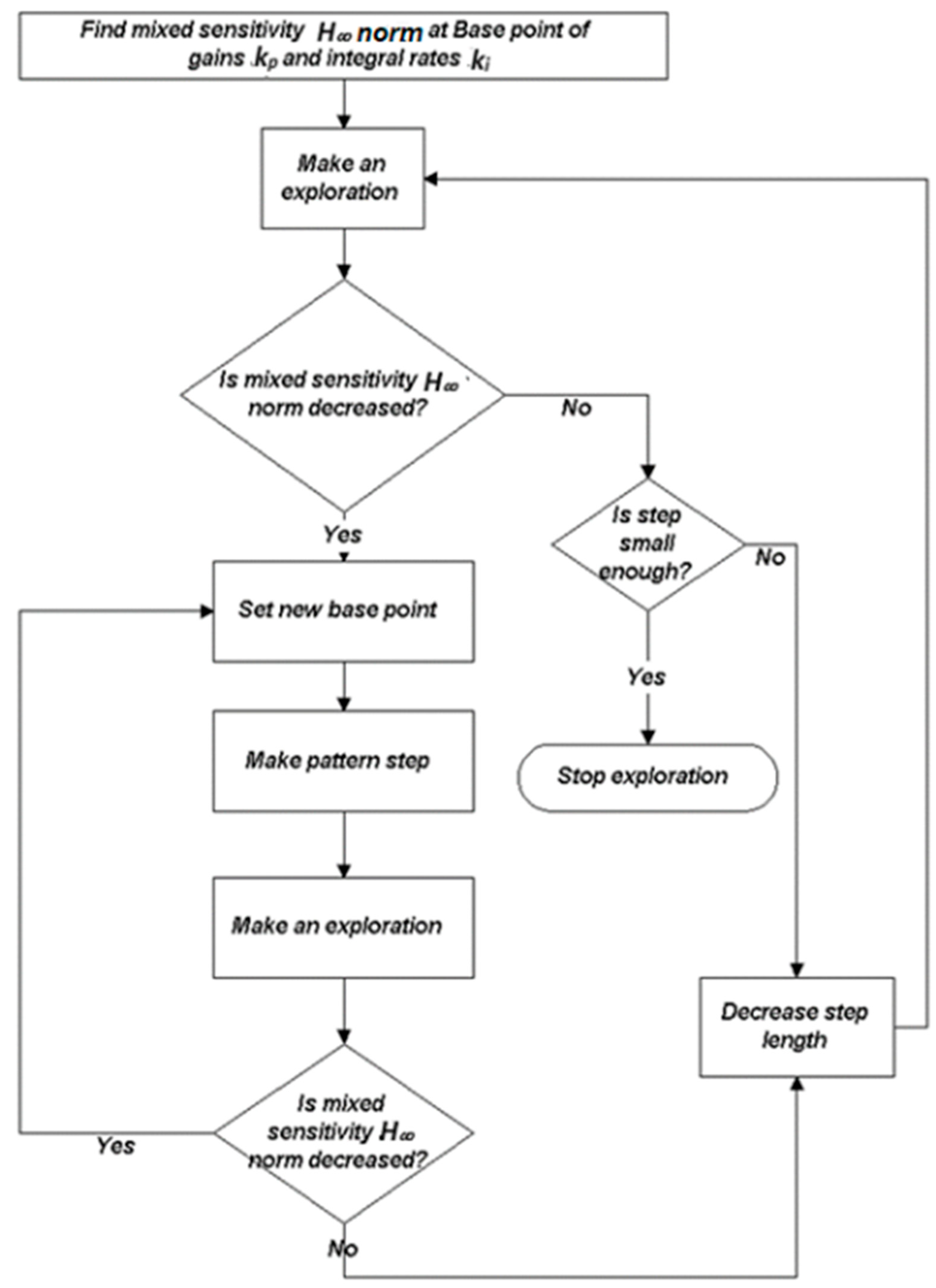
The flow chart of the pattern searches for finding the gain and integral rate, which results in a minimum
H∞ norm, is shown in
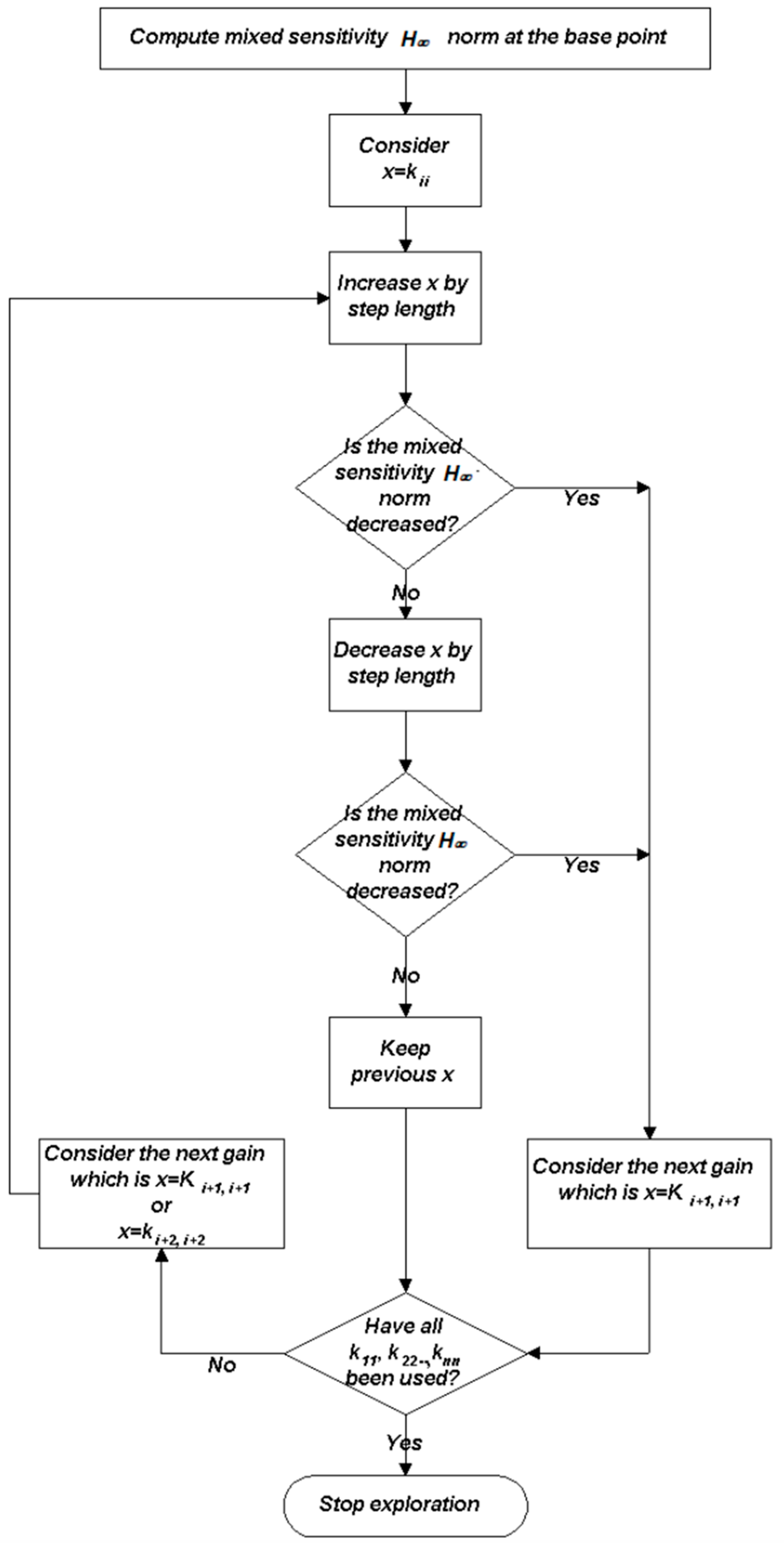
Figure 5. The main subroutine of the search is known as an exploration step about a base point, which, if successful, is followed by pattern moves. The details of the exploration procedures for finding the lower norm are described by the flow chart in
Figure 6. The bottom left block in
Figure 6 indicates that if the variable
is explored (bottom right block), then the next variable
(if any) should be explored. Otherwise (or), if the previous
is kept, then the variable
should be explored. The exploration step ends when all the variables are explored. Therefore, any exploration step in the Hooke and Jeeves optimisation method is deterministic.
An iteration procedure is also included in the robust control toolbox [
20] in MATLAB, based on the parameter
in (36), which is known as the
iteration. The main difference between the present approach and that of MATLAB is that in the latter, there is no choice in selecting the order controller structure. However, the required performance of the controller could be imposed by the weighting functions in (36) and (37). If a solution exists, then the program determines the specifications for the
H∞ controller. The final
value, obtained via the iterations, determines whether or not the desired sensitivity limit has been achieved.
For the following weighting matrices
a controller matrix consisting of PI diagonal elements was calculated using the Hooke and Jeeves search method.
Table 1 shows the search results including the initial PI parameters, the number of iterations, and the final resulting PI parameters, which are used to obtain the minimum rejection time when a step disturbance is imposed on the rotor system.
The resulting pre-compensator, which can achieve stability, together with the lowest possible norm, can be expressed as follows:
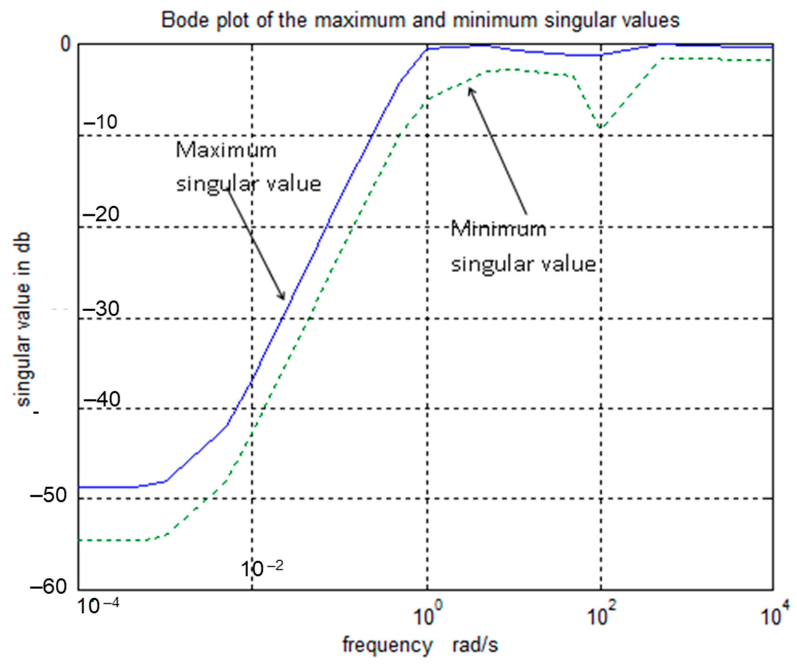
The maximum and minimum singular values of the
matrix are shown in
Figure 7, which shows that the upper and lower bounds are fairly close together. Both of the curves are below the 0 db line, as required.
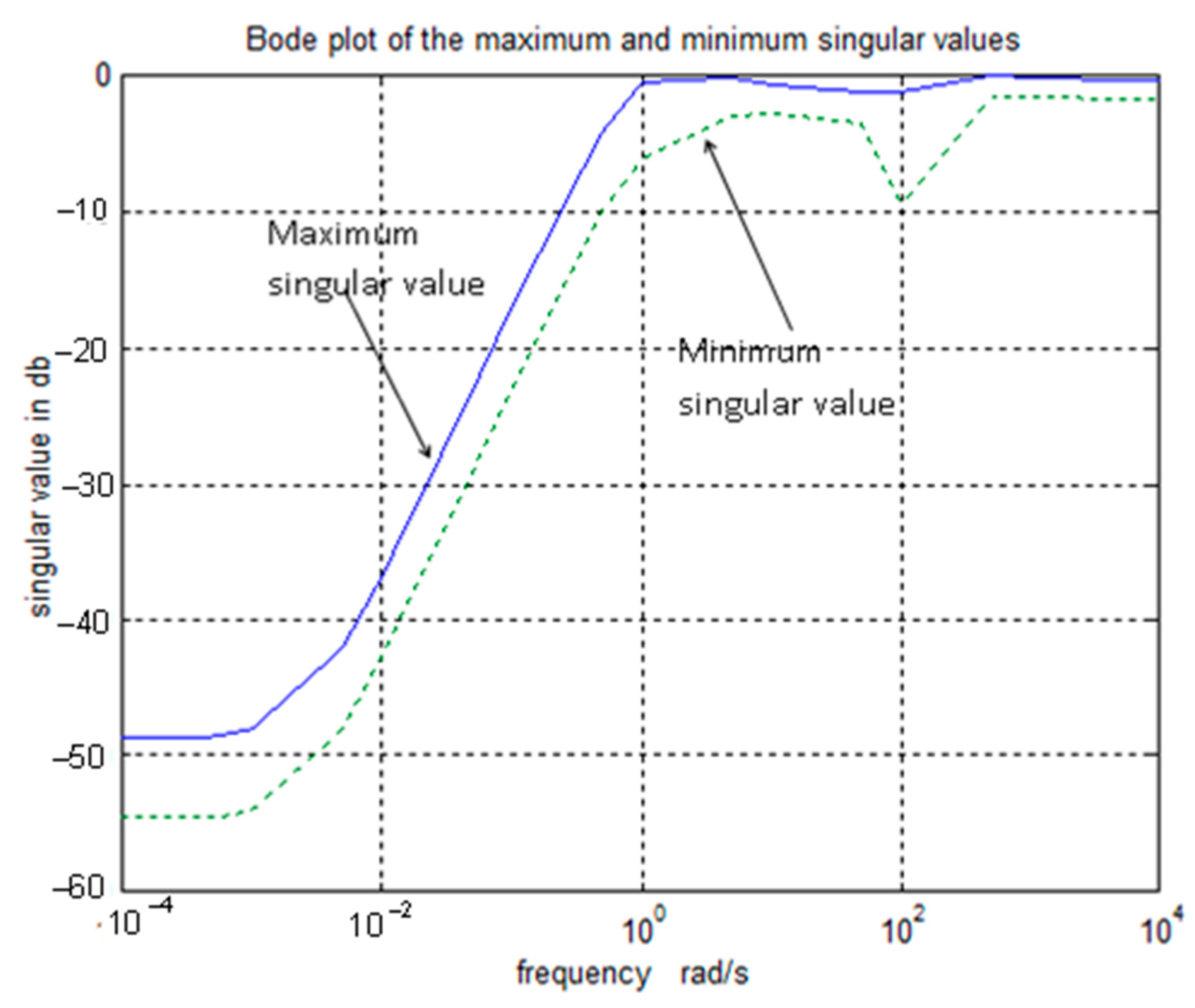
In
Figure 8, the Bode plot for the sensitivity matrix of the
H∞ optimal PI controller is shown, and this appears to be very satisfactory. The singular values are below 0 db for all frequencies, which is a significant achievement. Moreover, the condition number is very low because the maximum and minimum curves are very close together. This low condition number is not a result of optimisation. In fact, because the PI controller exhibits robustness, a low condition number is always associated with it.
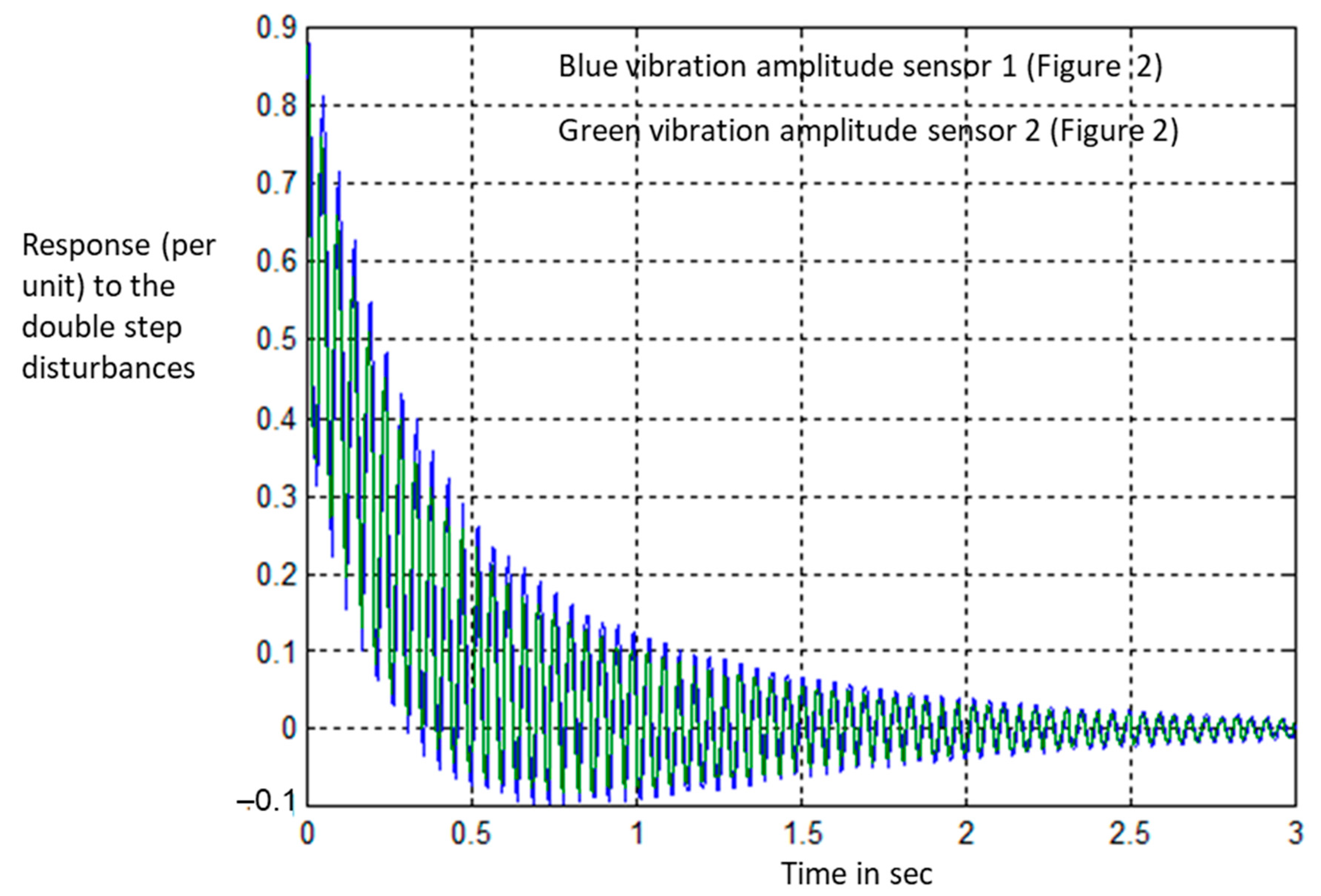
Although it seems that the above PI controller satisfies the
H∞ optimality condition, the simulation results show unsatisfactory responses, as indicated in
Figure 9. Regardless of minimising the cost function in (41), there are significant oscillations in the responses following double-step disturbances. The rejection time is also high, which is a sign of poor relative stability. This occurs because of the closed-loop pole and zero locations, which cannot be identified via the
H∞ optimality criteria.
It should be remembered that the PI controller in [
12], with following form
exhibits more appropriate responses as shown in [
12] but fails the
H∞ optimality test herein, with the resulting cost function of the following:
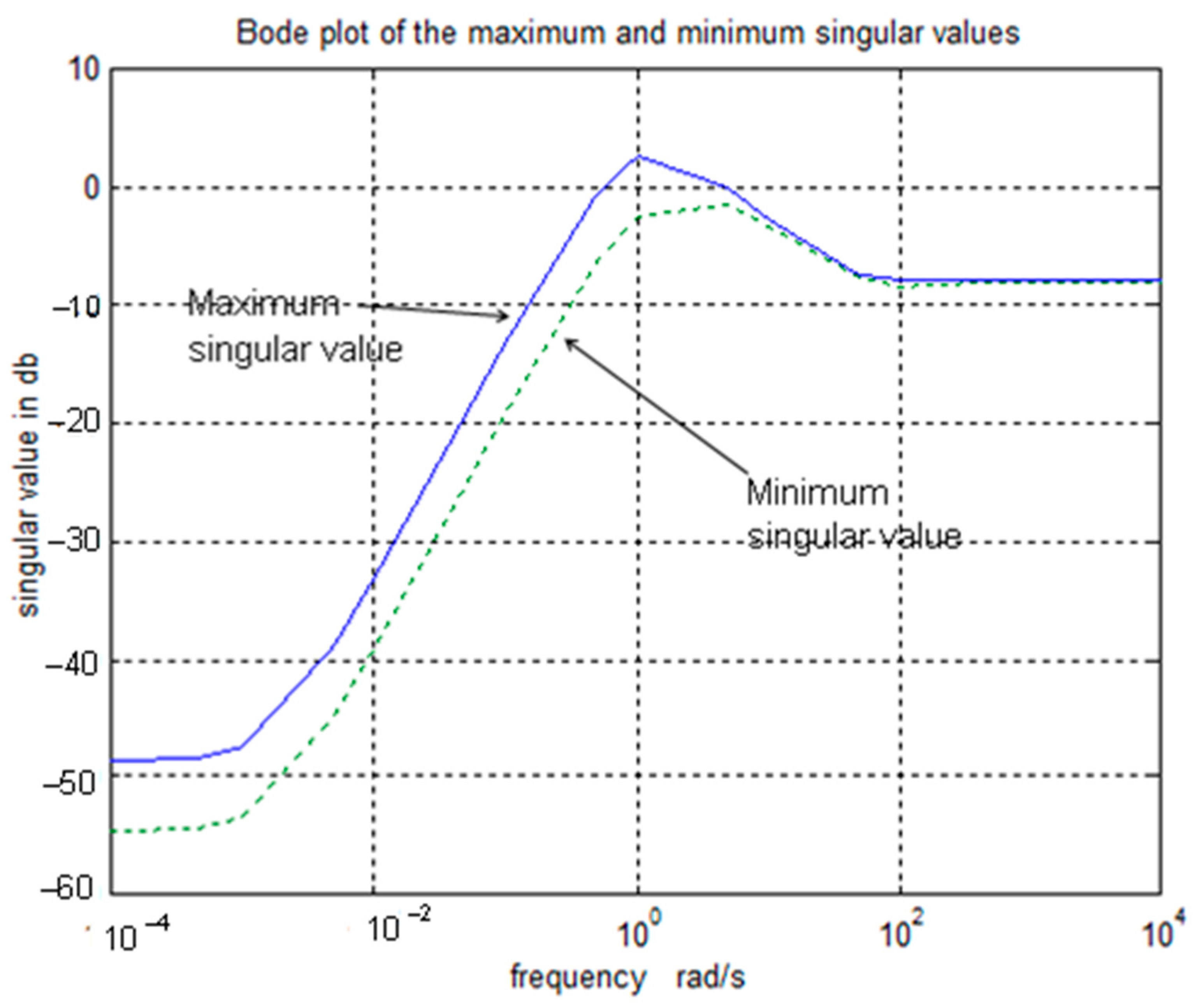
The Bode plot of the singular values of the cost function is shown in
Figure 10, where
reaches 2.7 db and seems to indicate failure but as shown in [
12] it works properly.
6. Performance Evaluation of the Minimum-Effort Controller
According to [
12], the minimum-effort controller
K can be expressed by the following:
In (48), the symbol >.< represents the outer products of
k(
s) and
h. The
consists of two simple time-delay filters given by (49), and
h is the gain vector given by (50). This makes the controller
strictly proper, i.e.,
In (49),
K = −1627 and
T = 17.11.
K and
T are found by optimisation techniques, according to the flow charts in
Figure 5 and
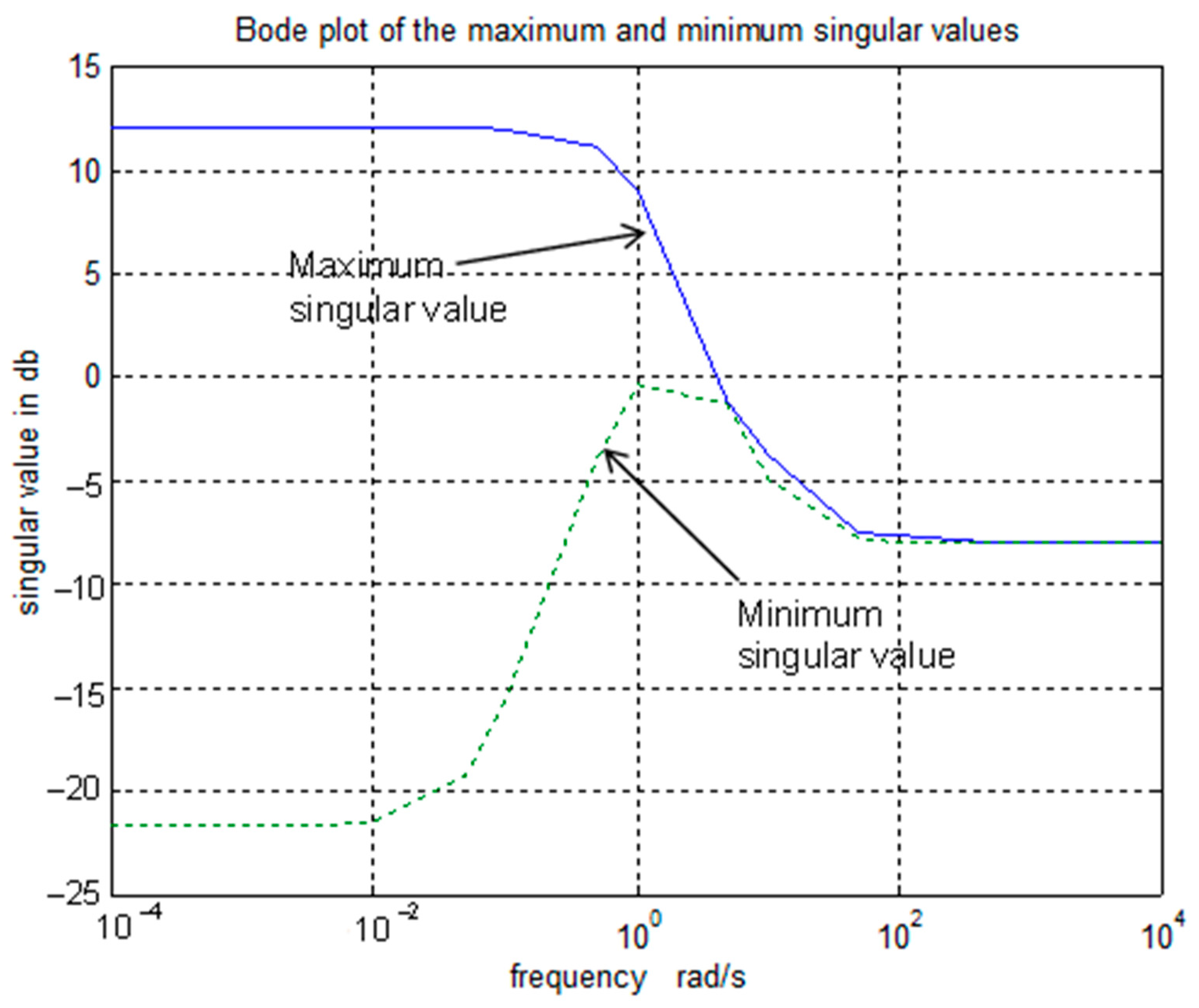
Figure 6. By considering the weights in (43) and (44), the maximum and minimum singular values of the
for the minimum-effort controller are drawn in the Bode plot of
Figure 11. It is shown that at frequencies over 5 rad/s, the maximum and minimum singular values drop below the 0 db line.
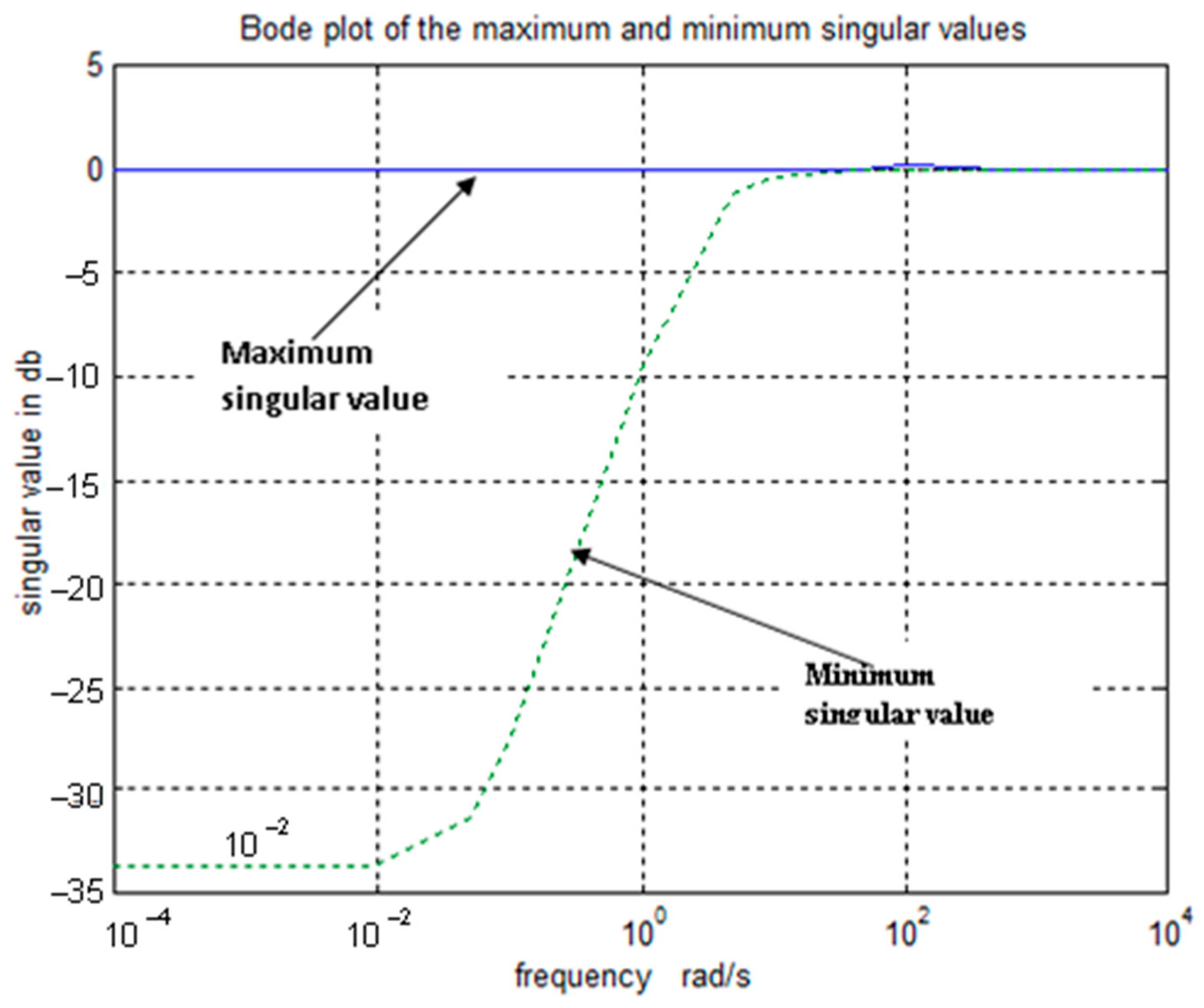
The singular values of the sensitivity matrix are shown in the Bode plot of
Figure 12, from which disturbance rejection, when using the minimum-effort controller, can be explained.
Figure 12 indicates that the maximum singular value is bounded by the 0 db line, while the minimum singular value, at lower frequencies, drops to –33 db.
This minimum singular value explains why such excellent step responses were achieved in [
12]. Therefore, any attempt to bring the maximum singular value below the 0 db line does not contribute to the performance of the controller.
Another excellent property is that both the maximum and minimum singular values converge at the line 0 db for the frequencies of interest, and this explains why the attenuation filter in the minimum-effort controller suppresses the oscillations significantly, with the lowest possible control effort.
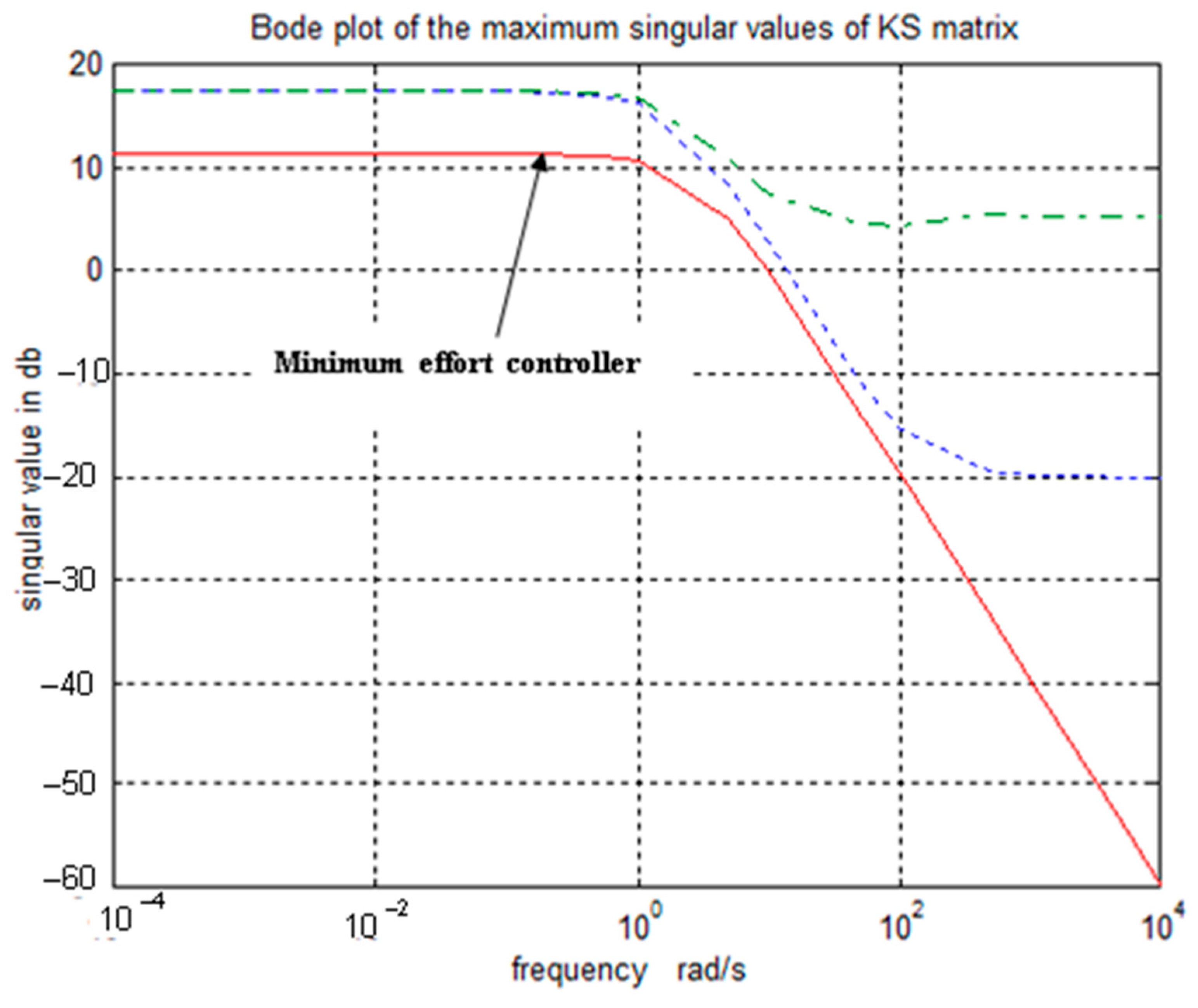
The performance of the minimum-effort controller can also be confirmed via the singular values of the control effort matrix
KS without any weight. In
Figure 13, the maximum singular values of
KS, for three types of controllers, are drawn for the purposes of comparison. It is seen that the maximum singular value of the minimum-effort controller indicated by the solid line is always below the curves for the PI controller of [
12], and the
H∞ optimal PI controller. Moreover, by using the minimum-effort controller, the control effort matrix
KS becomes singular, enabling the minimum singular value to be zero, scalar, or −∞ db and hence cannot be drawn for comparison purposes. Therefore, the lower bound of the control effort matrix
KS for minimum-effort controller is always lower than any other type of controller that can be implemented.
7. Design by Robust Control Toolbox
The MATLAB toolbox for robust control [
20] is based on
γ iterations and operates on the state-space time domain, where
γ is the coefficient of the weighting function in (36). The significant difference with our approach is that the parameters of the controller are fixed for each
γ and can be obtained from the state-space realisation of the plant, i.e.,
, which is defined by
Figure 3.
The theoretical framework for the development of the toolbox initiated by Doyle et al. [
21], who derived a formula for a family of
H∞ controllers for a given plant
, can be described by a minimal state-space realisation, in four blocks, as follows:
The Doyle formulas [
21] were based on several assumptions, the most significant being
Equation (52) does not include the general case. Later, Safonov et al. [
22] derived new sets of formulas for the case
with new assumptions, from which the robust control toolbox [
20] in MATLAB was developed. The algorithm results in an observer-based controller, generally with a higher degree than the open-loop-system
model. The lowest possible degree of the controller is equal to the plant degree
, which obviously depends on both of
and
.
This toolbox can also be employed for
H∞ mixed-sensitivity problems. Therefore, the results obtained would form a good comparison. For this purpose, we consider the same weighting matrix in (43) so that
and, to obtain a low-order, controller
The following procedures have been employed in our design using the robust control toolbox:
- I.
Start with a
γ value (21) and convert all the weighting matrices (53) to a state-space form [
23].
- II.
Convert the open-loop system
(7)–(10) to a state-space form [
23].
- III.
Assemble
and
to obtain the plant, i.e.,
(
Figure 4 and (28) and (29)), augmented in state-space form [
23].
- IV.
The conditions of the existence of an
H∞ optimal controller will be checked by the program, and if all the tests are passed, the state-space realisation of the controller will be produced by the program [
20].
- V.
When even one of the tests is failed, a new γ value is selected for the next trial.
- VI.
Finally, convert the state-space form to obtain a transfer function matrix description of the resulting successful controller [
23].
The conversion from state space to transfer function for multivariable systems herein is performed by the MFD toolbox in MATLAB [
23]. If
γ for this controller is too low, then the expected sensitivity function cannot be obtained by the controller and the performance would not be satisfactory.
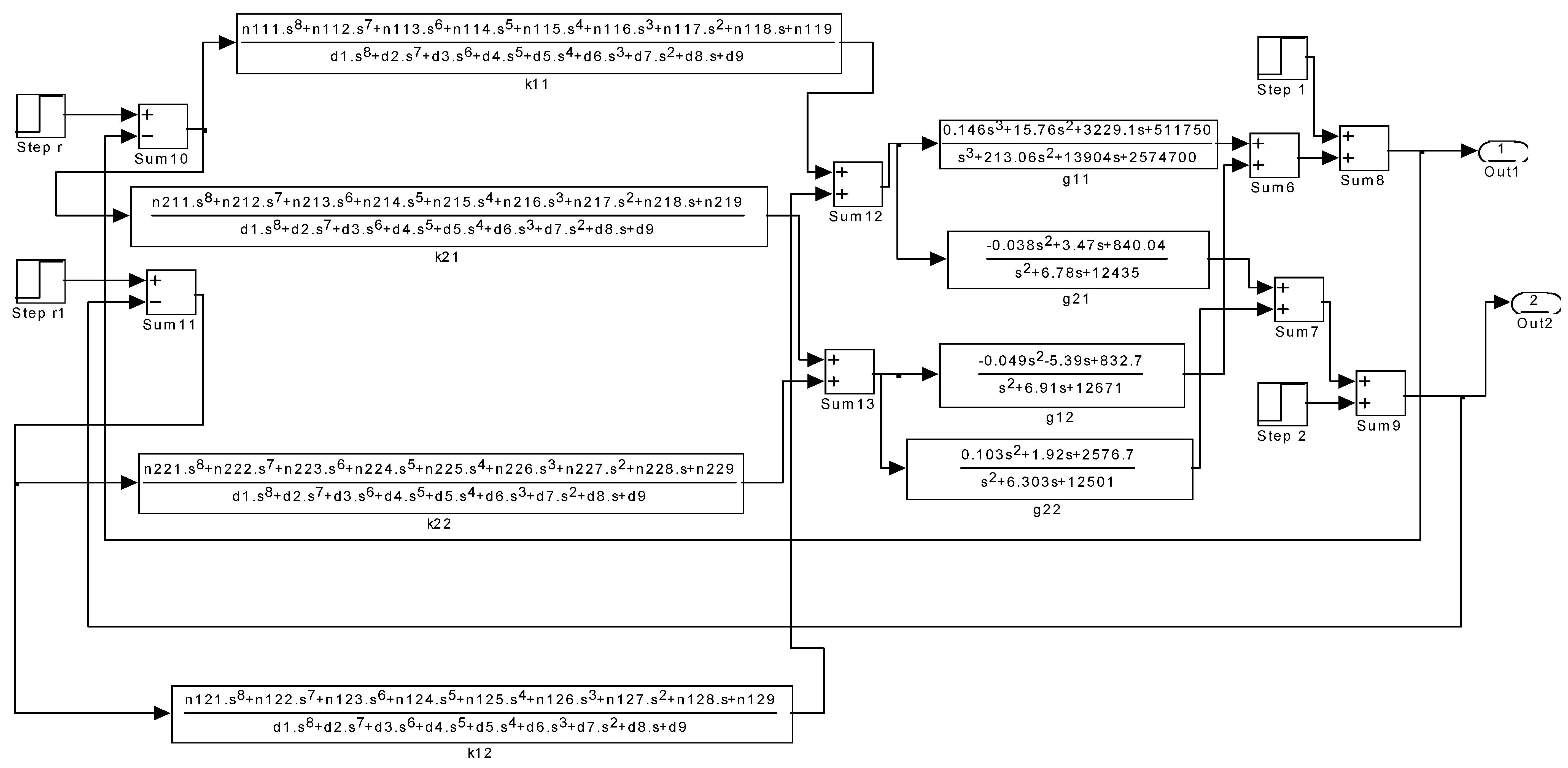
A starting value of
γ = 0.4, to satisfy the weighting function in (43), was selected. The first iteration was successful; therefore, all four controllers have been evaluated from this unique weighting matrix. The resulting eight-order controllers are described by the simulation block diagram in
Figure 14, in which the coefficients of the controllers are as follows:
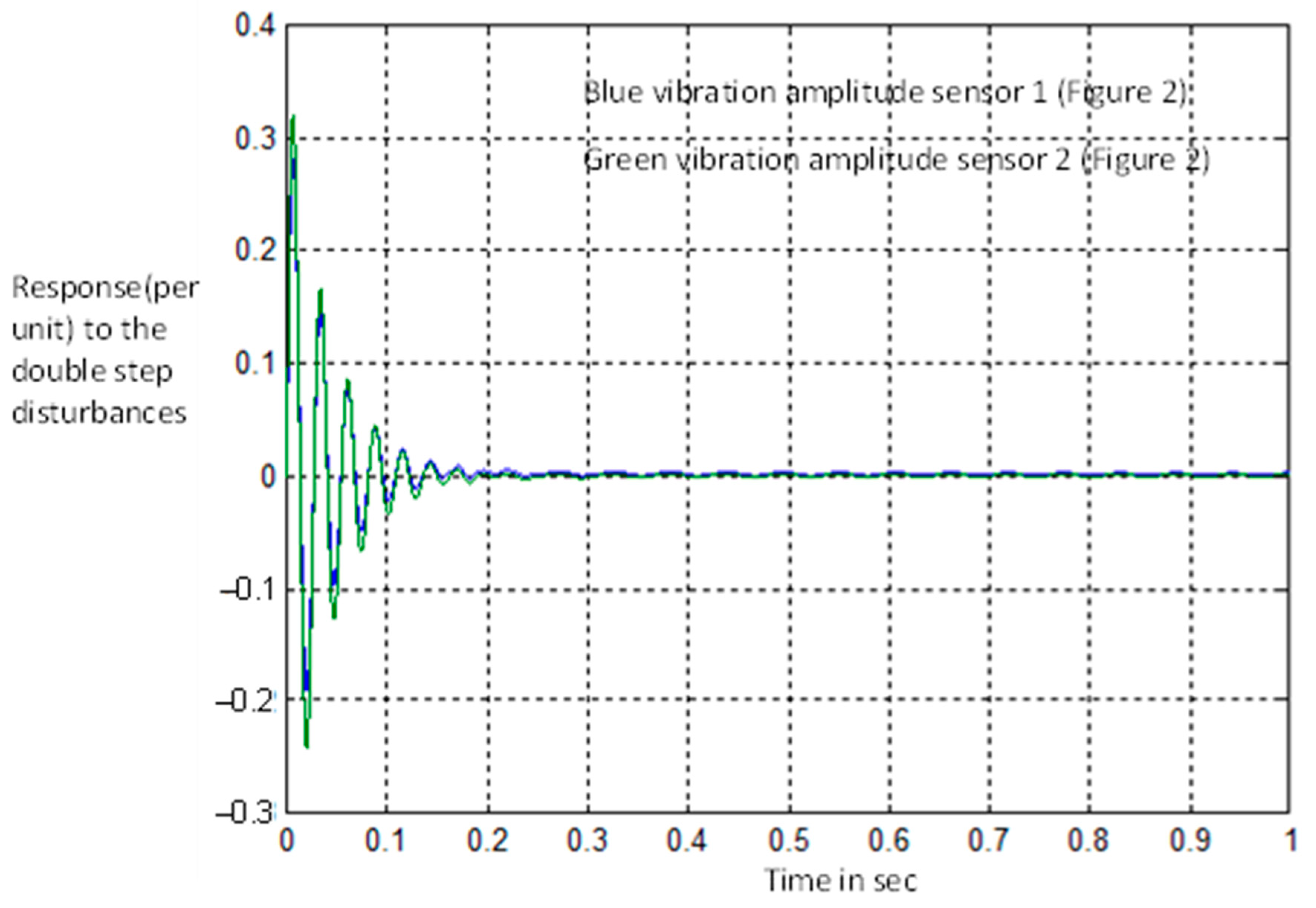
The response of the system to unity double-step disturbances is shown in
Figure 15, indicating a very low rejection compared with all other type of controllers, i.e., after a 0.3 sec full rejection has been obtained. The initial request for the sensitivity function imposed by
can in fact be satisfied by a 75% rejection, but full rejection was obtained. This controller is not practically realisable because of its higher order and because of the high gains required. There is also a maximum direct controller input–output transmission of a gain of 93,440, which would amplify the input signal noise, inhibiting effective system control. It should be noted that in
Figure 9 and
Figure 15, the response is per unit step, i.e., and it depends on the unit of the amplitude of the step disturbance.
As explained by
Figure 8, the PI controller can reduce the singular values to 0 db, but there is an unacceptable price to be paid for this in terms of the transient responses. This penalty cannot be avoided by the
H∞ optimal controller. The poor performance of the
H∞ optimal PI controller can be explained via
Figure 13, in which the maximum singular value of the control effort matrix is greater than the other two and is above the zero db line at all frequencies. The outcome is evident from the undesirable poor response in
Figure 9 with excessive oscillations.
Therefore, the shape of the sensitivity matrix’s singular values should not be misinterpreted, even if several H∞ norms have been minimised. A more accurate evaluation can be obtained by interpreting the singular value curves of the combined sensitivity and control effort matrix via a Bode plot, as in the case of the minimum-effort controller. In the final analysis, the controller must provide appropriate response characteristics in order to fulfil the dynamic and steady-state performance specifications, in addition to satisfying the H∞ optimality condition.
It can be suggested that
H∞ controllers are computational, and their performance is justified by simulation only (i.e., mathematically). In reference [
10], experimental results also show that, practically, there is no vibration suppression by
H∞ controllers.
8. Insights into Motivations and Methods in This Paper
The motivation for this theoretical article is a comparison of the performances of robust controllers that are designed both in the time and frequency domain. Such a comparison, particularly for the vibration control of long rotors, does not exist in the literature. This comparison is rigorous since the long rotor system requires multivariable models with a very high interaction index for their representation. Therefore, the level of rigorousness is high, therefore it requires a theoretical investigation.
It is shown that the time-domain controller design, by using the robust control toolbox, theoretically can work very well, and the settling time of the response reduces substantially when compared with controllers designed in the frequency domain based on the optimisation methods.
While the controllers found via the frequency-domain design can be simply structured, the H∞ controllers designed by the toolbox (i.e., time domain) exhibit a high order indeed, such that realisability is questionable. The higher order of the time-domain designed H∞ controllers are unavoidable, since they are observer-based controllers in the state space (big picture). The following table summarises the motivation.
Apart from
Table 2, the performance of the solutions can be measured by the
γ values in (21) in
Table 3 for the three types of controllers discussed in this article.
It should be remembered that in reference [
10], the rotor model is based on the mass, stiffness, and damping matrices of a rotor system. Such lumped models are easily convertible to a state-space model, but they are not accurate enough to represent a long rotor.
In this article, the model is obtained from a connection of the distributed parameter shafts to the lumped parameter disks and bearings and a multivariable transfer function matrix is accurately estimated for such a hybrid system. Therefore, by using the approach in this paper, apart from the accuracy of the model, it is also possible to compare the performance of controllers that are designed both in the time and frequency domain based on transfer function matrices. Such a comparison is the main purpose of this paper.
The dynamic stiffness K, D, and B partitioned matrices and their details in (1) and (2) express the dynamic model in this paper. They are represented in the s domain and include all the dynamic parameters of shafts, disks, and bearings. This builds Equation (1a), from which a transfer function matrix can be estimated. Therefore, the dynamic model is embedded in the elements’ transfer function matrix (5).
9. Conclusions
In this paper, the performance of two control strategies for disturbance rejection are evaluated by the H∞ optimality criteria. It has been shown that a PI controller can be computed with the lowest possible H∞ mixed-sensitivity norm and appropriate sensitivity matrix singular values. The resulting H∞ optimal PI controller enables full disturbance rejection with a slow oscillatory response. Thereafter, it can be concluded that the resulting poor transient responses may not be identified by the H∞ optimisation procedure.
An appropriate interpretation of the Bode plot singular values of the combined sensitivity and control effort matrix can be used to explain the performance shortcomings of this controller. Moreover, the performance of the minimum-effort controller, derived in [
12], is confirmed via a singular value analysis. It is demonstrated that the attenuation filter enables the maximum singular value of the sensitivity matrix to be bounded by the 0 db line, while the maximum singular value of the control effort matrix drops below the 0 db line. This indicates that a minimum-control-effort vibration suppression, together with noise attenuation, has been achieved.
Finally, the H∞ controller computed by the robust control toolbox in MATLAB results in rapid disturbance rejection, with the vibration amplitude diminishing to zero after 0.3 s. However, it would be very difficult to realise this eighth order controller in practice.


