Experimental Design Considerations for Assessing Atmospheric Corrosion in a Marine Environment: Surrogate C1010 Steel

Abstract

A rigorous assessment of marine atmospheric corrosion at a controlled NRL test site in Key West Florida was conducted. Certain factors which have been previously implicated in the literature as influencing the corrosion of engineering materials in atmospheric exposure were isolated and explored. In particular, the effect of sample size and orientation was explored. Low carbon steel (C1010) witness coupons were exposed in vertical non-sheltered, vertical sheltered, and tilted non-sheltered conditions. The effect of surface area on measured steel mass loss was also explored to identify the veracity of the so-called “edge effect”. Efforts were made to correlate meteorological atmospheric conditions (temperature, relative humidity, wind speed, wind direction, etc.) to the monthly assessment of corrosion damage. Results were assessed in terms of steel mass loss. Additive composite monthly corrosion damage tended to significantly overshoot the observed cumulative corrosion damage for samples exposed over the same period. This observation, among others presented herein, suggests that exposure of samples for less than 6 months is not an adequate predictor of long-term, natural exposure. Additionally, a smaller sample had a larger area-normalized mass loss than a larger sample. The influence of the sample edge (especially the bottom edge) was implicated in causing this difference.

1. Introduction

Materials exposed to the atmosphere tend to degrade in a process called atmospheric corrosion [1,2,3,4,5,6]. Many materials are impacted by exposure to water, salt, sunlight, temperature swings, etc. routinely present in atmospheric exposure, especially in a marine environment [1,2,3,4,7,8,9,10,11,12,13]. Field exposures differ markedly from laboratory exposures due to the complex tapestry of variables that are both numerous and not experimentally controlled. For this reason, it can be difficult to correlate various environmental parameters to observed corrosion performance, whether in isolation or in concert, though many excellent investigations have undertaken this very objective [1,2,3,4,8,9,10,11,12,13].

Briefly, several factors have been noted to affect atmospheric corrosion. In any corrosion process, thermodynamically viable anodic and cathodic reactions must have successful electron transfer while maintaining electroneutrality in a conductive electrolyte. Viable anodic reactions depend on the material in question, salinity, pH, passivity, scale formation, etc. Viable cathodic reactions are available from atmospheric reagents characteristic of a given site. Electron transfer occurs proximately between anodic and cathodic reagents or remotely between anodic and cathodic sites if mediated through the conducting metal substrate. In the atmosphere, the corrosion process occurs in some thin electrolyte film [3,5,6,11,12,14,15,16,17]. The thin film can originate naturally from and persist during precipitation (rain, drizzle, etc.) and condensation (dew, fog, etc.). However, most of the time, the film forms and persists because of salt deliquescence at sufficiently high humidity. Deposited salt on a material surface will equilibrate with the water in the air to form an aqueous, deliquescent electrolyte film for relative humidity at or above the deliquescence point. The concentration and thickness of the deliquescent film depends not only on relative humidity but also on the identity and deposition density of the salt [5,18,19,20]. This in turn influences the corrosion process. The presence of salt on the surface of a material is strongly correlated to factors such as precipitation and ambient aerosol concentration, which in turn depends on geography, proximity to salt bodies, wind, humidity, etc. [4,9,10,13,21,22,23,24].

With so many uncontrolled and fluctuating parameters affecting atmospheric corrosion at once, it is necessary to simplify the assessment of corrosivity by means of a standardized deployment procedure. This increases the reliability of atmospheric testing and facilitates the comparison of various sites against each other for environmental indexing severity rankings. Standards such as ASTM G4 [25], ASTM G50 [26], ISO 9223 [27], ISO 9224 [28], and ISO 9225 [29] cover details pertinent to sample deployment and assessment of corrosivity. Factors such as exposure rack design, sample size, exposure angle, replicate count, surface preparation, environmental monitoring, etc. are considered. Standards also recommend having control panels against which to make corrosion assessments. Proxy, or witness, coupons are commonly deployed to assess the relative corrosivity of environments. One common proxy is low carbon steel.

Low carbon steel is used as an atmospheric corrosion proxy for several reasons. First, as a ferrous alloy, it indicates how other ferrous alloys may behave in a given environment. Second, the corrosion morphology is general (uniform) attack, meaning that damage is experienced globally across the whole sample without the added complexity of accounting for stochastic processes such as pitting. Third, the corrosion rates are generally large enough that significant results can be measured in short time frames and corrosion rate can be determined from simple mass loss procedures.

The development, promulgation, and adherence to standards is important for reducing error, increasing accuracy and precision, and cross-referencing of results. Unfortunately, ambiguities can exist, or best practices develop over time and adherence dwindles. Often, the rationale for various specifications are known only to the drafting committee. Sometimes specifications are listed as recommendations, leaving room for variation from one study to the next. Finally, it is sometimes advantageous to diverge from standards in order to probe the effect various alterations have on the corrosion response to better understand the atmospheric corrosion process. This investigation will revisit certain experimental design factors to probe their influence on the corrosion process. Factors such as sample size, sheltering, and tilt will be assessed using low carbon steel C1010 proxy samples.

2. Materials and Methods

2.1. Samples

The witness coupons consisted of C1010 low carbon steel deployed in triplicate. The C1010 (notated as Fe) is a common proxy sample for steels in general (although it is starkly different from other classes of steel such as stainless, cast iron, or high strength steels). The steel coupons had a glass bead blasted surface and were either 3″ × 3″ × 1/16″ (to be referred to as Wide) or 0.5″ × 3″ × 1/16″ (to be referred to as Thin) in dimension. Samples had two 3/16″ diameter mounting holes located 1/4″ off the edge and centered in the middle of the samples.

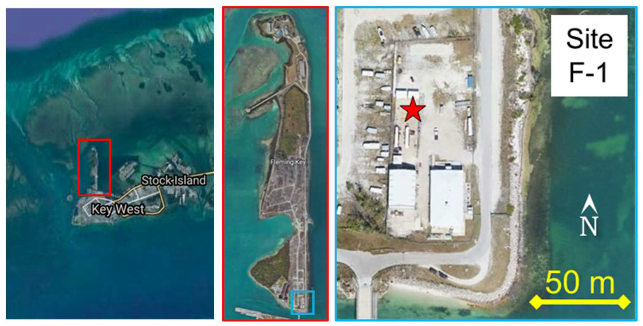
2.2. Exposure

NRL Key West is a state-of-the-art testing facility located on Fleming Key within the Naval Air Station. The facility is equipped for structural testing, coating application, and outdoor exposure (both marine submersed and marine atmospheric). Its location at the end of the Florida Keys makes it an ideal test site for isolating atmospheric effects in the absence of influences from industrial or continental containments. There are principally two sites at the NRL Key West facility, F-1 and F-14. An overview of the facility is shown in Figure 1.

For this analysis, exposures of C1010 steel coupons were conducted from 28 August 2014 through 28 August 2015 at the F-1 site. Samples were deployed in three conditions, as shown in Figure 2. For the Non-Sheltered (N) condition, samples were oriented vertically with respect to the ground (90° off the horizon) and were not sheltered overhead from precipitation or solar radiation. For the Sheltered (S) condition, samples were oriented vertically but were sheltered from the direct impingement of precipitation by a 4-inch acrylic overhang (above) and sidewall (left and right). For the Tilted (T) condition, samples were oriented at a slant, 45° off of the horizon and were not sheltered in any way. All samples were facing South, the direction of maximum solar impingement. The Thin samples were oriented with the short dimension (0.5″) parallel to the ground. Samples were mounted so that the mounting holes were located one over the other.

Samples were exposed both cumulatively and monthly. Cumulative samples (C) were pulled each month which had been exposed from the beginning of the deployment until the time of retrieval. Monthly samples (M) were pulled each month which had only been exposed for the month prior to the time of retrieval and which were replaced by fresh samples to be exposed only over the course of the subsequent month.

Meteorological data were collected on-site from a collocated weather station every half hour. Common environmental parameters were measured such as temperature, relative humidity, wind, precipitation, etc. Some specialty parameters were calculated such as wind power, which is the product of the mean half-hourly average wind speed and the length of time the wind was blowing from a given direction summed together for each month period. For example, total wind power was calculated indiscriminately of wind direction, whereas Easterly wind power was collated when the wind was blowing between 45 and 135 degrees. Rain days are simply the number of days which had rainfall each month. The solar irradiance is the total sum of mean half-hourly average irradiance recorded for each month period. Three uncoated time of wetness sensors were also deployed for an overlapping portion of the sample exposure in each of the three conditions: Non-Sheltered, Sheltered, and Tilted. The time of wetness sensors measured the resistance between two gold interdigitated electrodes, which correlates to the thickness, concentration, and coverage of electrolyte films on the surface [11,30]. All resistance measurements were collected, and the 3rd quartile value was found to be 1977 kΩ. Resistances below this threshold were binned as “wet” values. The time of wetness is the percentage of time the sensors recorded resistance values below this “wet” threshold. The meteorological data are available publicly from the Open Science Framework data repository at DOI 10.17605/OSF.IO/SGEUN, Supplementary Materials.

The Wet Candle technique was also utilized to determine the relative chloride deposition flux at the site on a monthly basis following ASTM G140 [31]. Correlations can be made between chloride deposition flux and corrosion damage. The procedure for candle deployment and analysis follows best practices for maximum fidelity [32,33].

2.3. Testing and Analysis

Mass loss measurements were collected from the C1010 low carbon steel coupons by recording the initial mass before deployment, the resulting mass after exposure, and the final mass after removal of the corrosion product. Accumulated corrosion product was removed via glass bead blasting in order to isolate the metallic substrate remaining after the exposure. Then, the area normalized mass loss density (grams per meter squared) was calculated. The area of each steel sample type was calculated considering all of the exposed surfaces of the sample (six faces of coupon) and correcting for the area not accounted for by the mounting holes but including the area along the side wall of the mounting holes. If the percent deviation ([standard deviation/average] × 100) of a triplicate set of measurements was higher than 25% then the replicate which was furthest removed from the arithmetic mean was excluded in analysis (Larger deviations within a triplicate set were observed for cumulative samples. This suggests that data scatter maybe introduced as part of the process of removing the corrosion scale from longer exposed specimens. For sample TM 1.8, this data-truncating step was repeated twice before the percent deviation was below 25%, meaning only the median replicate value was used). Mass loss data are publicly available from the Open Science Framework data repository at DOI 10.17605/OSF.IO/SGEUN Supplementary Materials.

Where applicable, a trendline is overlaid on data to provide a guiding trace of the general trend. The trace is plotted using a basis spline fit to the data which fit the data to an objective function where no inference is applied as to the mathematical relationship between dependent and independent variables. Conversely, where a linear trend is assumed and plotted, the Pearson’s correlation coefficient (ρ) is included to provide an indication of the fittingness of the assumed linear relationship. These linear fits and Pearson’s correlation coefficient calculations were made for the entire population of available data. Values near 1 or −1 indicate a strong correlation between the two variables. For the purposes of this analysis, positive or negative values of ρ ranging in magnitude from 0.00–0.25 indicate no correlation, 0.25–0.50 indicate moderate correlation, and greater than 0.50 indicate strong correlation. Finally, data are plotted for two different cases. In the cumulative case, for example, the sample was subjected to the full ten months of exposure. For the additive composite case, for example, data values from ten individual 1-month exposures were added together to approximate the mass loss of the cumulative 10-month case over a common period of time.

3. Results

3.1. C1010 Steel Mass Loss

The mass loss density measured for the Wide samples is reported in Figure 3. It is first noted that the composite addition of monthly mass loss values (patterned and colored bars) is greater than the mass loss observed for the cumulative samples (solid grey bars) for every condition. As the exposure continues, the difference between the additive composite monthly values and the cumulative values increases. Wide Non-Sheltered and Sheltered condition have essentially similar behavior, while the Tilted is markedly different (higher mass loss) as seen in Figure 3d.

Similarly, Figure 4 shows that composite monthly mass loss values are greater than the equivalent cumulative mass loss values for the Thin samples as well. The three conditions are now closer to each other in mass loss, but a trend is still distinct, especially at longer times, with Tilted > Non-Sheltered > Sheltered. This trend is also distinguishable in the Wide samples, if only barely (Figure 3).

Figure 5 provides a perspective on the effect of Wide vs. Thin steel. Comparing equivalent conditions side-by-side, the Thin steel has a higher mass loss density than the Wide. This is despite having corrected or normalized for the differences in the area between the two samples (the mass loss density is reported in g/m²). This behavior is less obvious for the Tilted case but still discernable. The Thin steel has a 15% greater mass loss than the Wide steel for the Tilted condition, whereas the Non-Sheltered and Sheltered cases exhibit 45% greater mass loss for Thin than Wide (Figure 5b).

Figure 6 provides a perspective on the effect of elapsed exposure time by assessing the difference between a cumulative measurement and a composite monthly measurement. Naturally, for the first month the difference between cumulative vs. composite is low because there is no real distinction in the first month. Between two and ~six months of exposure the difference between composite and cumulative is relatively constant. However, after six months the difference between the composite and the cumulative mass loss increases at a constant rate. This general trend is consistent across the three conditions and for Wide and Thin samples (Figure 6). For Wide samples, the effect is most prevalent for the Sheltered condition, then Non-Sheltered, followed by Tilted. The three conditions are much more similar for the Thin samples.

Figure 7 shows monthly mass loss values over the course of the year to give an indication of the seasonal variability in the corrosion severity of Key West over this period. Every condition is reported for Thin and Wide samples. Since the common practice in the community is to expose Wide geometry samples in the Tilted orientation, a trace is included for that specific control case in black (Figure 7). The general trend outlined by the trace holds for the other conditions and geometries as well. Essentially, the mass loss is highest in the late spring/early summer (Apr, May, Jun) and lowest in late summer/early fall (Jul, Aug, Sep, Oct).

3.2. Meteorological and Environmental Parameter Correlation

Meteorological and environmental data were collected contemporaneously with sample exposure. Chloride and sulfate deposition flux as measured by the Wet Candle technique [32,33] is reported in Figure 8a. The chloride data are fairly scattered in 2014 but becomes more controlled in 2015, showing a higher propensity for chloride deposition in late winter/early spring (Jan–Apr) and a lower propensity for deposition in late summer/early fall (Jun–Oct). Chloride deposition is closely correlated to corrosion risk [7,8,13,20,34,35,36]. The deposition of chloride onto these surfaces is dominated by dry deposition of sea spray aerosol for this marine coastal environmental [2,4,9,13,23,37,38,39].

Sea spray aerosol flux into the atmosphere from the ocean results from agitated sea interfaces [2,4,21,22,37]. Wave crashing on the shoreline is one major source. White-capping from wind-ocean shearing is another. As such, the mean average wind speed correlates strongly to the observed chloride deposition flux on a monthly basis throughout the length of this campaign (Figure 8b).

Gold interdigitated time of wetness sensors were deployed in the same three conditions Non-Sheltered, Sheltered, and Tilted to capture the differences in the microenvironment on the surface wetting. In all cases, the surface was most frequently wetted during the colder half of the year spanning from November to April (Figure 8c). The Sheltered condition generally yielded a higher percentage of time in which the sensor was in a wetted state, while the Tilted condition yielded the lowest time of wetness. Time of wetness, in part, is an indication that the surface of the sensor (and presumably that of a sample as well) is characterized by a thin electrolyte film of sufficiently high conductance to be considered “wet” [11,30,40]. The film may originate from precipitation, condensation, or deliquescence. Deliquescence is humidity dependent, so the time of wetness correlates strongly to the mean average relative humidity (Figure 8d).

Figure 8e gives a seasonal outlook on some of the environmental parameters that are known to both impact corrosion and vary from season to season. Key West is a tropical savannah climate (Köppen Code Aw [41]) characterized by a dry winter season and a wet summer season (https://www.weather.gov/key/climate, accessed on 24 October 2022), as shown by the total rainfall intensity curve (Figure 8e). The onset of the wet season coincides with an uptick in the Easterly wind power, which remains elevated throughout the wet season. The chloride deposition intensity also tracks well with the trend in the Easterly wind power profile. Included is the seasonal variability in the monthly mass loss for the wide tilted steel sample. The mass loss is greatest during the transition from the dry to wet season (Figure 8e). The mass loss is generally higher in the dry season than in the wet season. Steel mass loss tracks well with both the chloride deposition intensity and also the time of wetness (which is highest in the dry season and lowest in the wet season). It should be noted here that the descriptor “wet” or “dry” refers specifically to the amount of precipitation, not to the condition of a surface, which may be wetted for reasons other than precipitation, such as deliquescence, dew, or sea spray.

Chloride is known to be a key facilitating agent in the atmospheric corrosion process [7,8,20,34,35,36,42]. The correlation between steel mass loss and chloride deposition is shown in Figure 9. Generally, more chloride deposition correlates to more mass loss, especially for the Tilted condition but very weakly to the Sheltered condition.

Several environmental parameters have been correlated to the mass loss density observed for Wide steel (Figure 10). A moderate to strong correlation exists between solar irradiance and steel mass loss (Figure 10a). The number of days in a month which experienced rain was correlated against steel mass loss (Figure 10b). Generally, a higher occurrence of rain results in less mass loss, except for the Sheltered condition, which is indifferent to the effect of rain days.

The role of the wind was assessed against steel mass loss as well (Figure 10c). The mean average wind speed correlated strongly to mass loss except for the sheltered condition in which it did not correlate. The trend did not change when considering total wind power instead of mean average wind speed (Figure 10d). However, there was a significant change when considering Easterly wind power, as the correlation became very strong (Figure 10e), especially for the Sheltered condition, which was indifferent to the other wind parameters. The correlation to the time of wetness was moderate to strong; however, the correlation indicates that for the Sheltered and Non-Sheltered conditions the two variables were independent of each other given the slope (Figure 10f). Assessment in terms of time of wetness was correlated directly between samples and sensors exposed in the same condition. Unfortunately, there were limited data available to correlate time of wetness to the Non-Sheltered and Sheltered conditions.

Pearson correlation coefficients from the assumed linear trends fitted for the two-variable relationships shown in Figure 9 and Figure 10 are given in

Table 1. Pearson correlation coefficients of the (assumed linear) relationship between Wide steel mass loss density and various environmental parameters. Cells are color-coded as follows: ρ < −0.5 (dark red), −0.5 < ρ < −0.25 (light red), −0.25 < ρ < 0.25 (light grey), 0.25 < ρ < 0.5 (light green), 0.5 < ρ (dark green).

	Solar Irradiance	Rain Days	Wind Speed	Total Wind Power	Easterly Wind Power	Time of Wetness	Chloride Deposition Flux
Non-Sheltered	0.65	−0.48	0.50	0.46	0.68	0.77	0.25
Sheltered	0.77	−0.02	0.11	0.03	0.70	0.45	0.11
Tilted	0.36	−0.48	0.58	0.55	0.54	0.25	0.48

The cells are color-coded to indicate the strength of the correlation. Visually it can be seen that there is the strongest positive (proportional) correlation for Easterly wind speed, solar irradiance, and Time of Wetness (in that order) and the strongest negative (inverse) correlation for rain days.

4. Discussion

4.1. Sheltered vs. Non-Sheltered

It must first be noted that the descriptor “Sheltered” in this context means that the sample was sheltered from the impingement of precipitation by the 4 inch acrylic overhang and sidewalls. The shelter was meant to prevent wet deposition on the surface, or deposition facilitated by precipitative action. Possibly some wet deposition may certainly have happened during stronger and windier precipitation events. The sample was not intended to be sheltered from the impingement of solar radiation. In fact, the material for the shelter was chosen for its transparency to ultraviolet light. There may be a slight reduction in the total intensity, but the design was for ultraviolet radiation to still play a role in the corrosion process for all conditions. For this reason, it is not surprising to see that the steel mass loss was sensitive to solar irradiance regardless of the exposure condition (Figure 10a).

The mass loss results were very similar for the Sheltered and Non-Sheltered conditions (Figure 3d and Figure 4d), with the Sheltered samples having slightly less mass loss. Sheltering may have affected the prevalence for salt deposition onto the surface. Wind was a strong determinant for steel mass loss except for the Sheltered condition. There was no correlation between Sheltered mass loss and wind until Easterly Wind Power was used specifically, at which point there was a very strong correlation (Figure 10e). For the Key West site, the Easterly wind has been found to correlate to corrosion damage because transport of sea spray aerosols from their source to the site aligns in that direction. The effect of sheltering seems to be diminished when considering the potency of salty Easterly winds. Additionally, salt deposition does not only occur from lateral transport due to wind, but also from vertical transport due to gravitational settling. The sidewalls and the overhang together reduce the efficiency of salt deposition onto the vertical Sheltered steel.

4.2. Tilted vs. Non-Sheltered (Vertical)

The steel mass loss results show a prominent effect due to tilting (Figure 3 and Figure 4). The Tilted condition resulted in much more mass loss than the Non-Sheltered condition. In terms of precipitation and solar impingement, the Tilted condition is most favorably oriented to maximize their effect. The maximum solar radiation flux on a sample occurs for an exposure angle (with respect to the horizon) equal to the latitude at which the sample is exposed. Since the Key West site is situated at a latitude of ~24.57, the solar flux to the (45°) Tilted sample is much greater than the (90°) Non-Sheltered sample since it is closer to the maximum flux angle of ~24.57°. Presumably, a similar concept holds for precipitation, as the flux of rainwater to the sample is greatest for a (0°) horizontal sample and least for a (90°) vertical sample. The Tilted condition is again, more favorably oriented than Non-Sheltered to experience the effect of precipitation. Similarly, the gravitational settling of salt-laden sea spray aerosols is expected to be greater for the Tilted condition than the Non-Sheltered condition. Since the deposition of salt and the flux of solar radiation is expected to be greater for the Tilted condition, and both of those factors correlate with greater mass loss, it is reasonable to see why the Tilted condition had more mass loss than the Non-Sheltered condition. Rain occurrence was inversely correlated to mass loss, so it is not clear why the Titled condition would have more mass loss than the Non-Sheltered in that regard, unless the influences from salt deposition and solar impingement outweigh the rain influence.

4.3. Sample Size: Thin vs. Wide

The Thin geometry consistently saw 15–45% greater mass loss values than the Wide geometry (Figure 5b), despite the values being area-normalized (grams per meter squared). We hypothesize that the discrepancy in the mass loss values is due to an edge effect whereby the edge of a sample corrodes in a manner inconsistent with the rest of the bulk, boldly exposed surface of the sample. In this way, different-sized samples may yield different area-normalized mass loss values if the effect of the edge is not taken into consideration. If correct, then the edge effect hypothesis would suggest that smaller samples tend to yield higher area-normalized mass loss values than larger samples (assuming that the edge corrodes more than the bulk). It is possible that there is some size threshold above which the effect of the edge is negligible compared to the contribution from the rest of the bulk. This would be the ideal steel proxy sample size to use for environmental severity index testing.

The origin of the edge effect may arise from several mechanisms. First, the edge contains a sharp geometry, for which corrosion attack may be more prevalent. This could possibly be due to curvature effects at the edge in a manner analogous to nanoparticle electrochemical dissolution [43] (though certainly less potent for the machined edge). Second, there may be residual stresses present at the edge due to the machining required to fabricate the sample that increase the propensity for corrosion attack. Perhaps other microstructural effects exist at the edge to due fabrication (cold working) as well (grain size, grain orientation, etc.). Additional mechanisms can be postulated by considering the condition of the samples upon extraction from the atmospheric exposure. The bottom edge of the steel samples commonly consists of a bright orange band of corrosion product, whereas the rest of the sample consists of a dark red corrosion product. This is exhibited in Figure 11 for 12-month samples in the Tilted and Non-Sheltered condition. It is possible that the edge effect is specifically a bottom edge effect which arises from the following mechanisms in addition to the two postulated already. Third, a differential aeration cell may be established between the edge and the bulk. If the bottom edge of the sample consists of a bead of electrolyte pooled up at the edge due to capillary effects and the rest of the sample consists of a thin deliquescent electrolyte film, then the thin film may allow faster oxygen uptake and transport than the thicker bead at the bottom edge. In this instance, the bottom edge would be activated as an anode while the rest of the bulk would be a cathode. Fourth, perhaps as the sample dries out after a wetting event or when the relative humidity drops below the deliquescence point, the bottom edge is the last portion of the sample to dry. If this were the case, then the bottom edge would be wetted for longer amounts of time than the rest of the sample and would corrode more simply because of a difference in localized time of wetness. Fifth, perhaps as the sample dries out and the electrolyte pools up at the bottom edge it also wicks the salt on the surface along with it. In this way, the bottom bead of electrolyte also becomes saltier and saltier as it consolidates on the edge. Salt concentration is known to scale with corrosion damage [1,4,36] and salt wicking at the bottom edge may lead to more attack at that edge. Evidence for some sort of capillary effect of the size of a bottom bead of electrolyte is observed by comparing the Tilted to the Non-Sheltered (vertical) samples (Figure 11). The bright orange band on the bottom of the Tilted monthly sample is thicker than for the Non-Sheltered monthly sample. The 45° angle of exposure for the Tilted sample likely resulted in a thicker bead of electrolyte at the bottom of the sample than the vertically exposed Non-Sheltered sample. At this time, it is unclear why the difference between the Wide and Thin Tilted samples was smaller than for the Sheltered or Non-Sheltered samples.

A generic edge effect may be mitigated by deploying samples of larger face area to edge perimeter ratio. Larger samples increase the area to perimeter ratio, as do circular, or disk, samples [25]. A machining treatment to the edges has been proposed to eliminate the effects of possible stress or cold-working [25]. A bottom edge effect specifically may be mitigated by orienting samples such that the shortest edge is along the bottom (for rectangular plates, for example). Anecdotally, the two sizes selected for this investigation (0.5″ × 3″ and 3″ × 3″), are commonly used for atmospheric exposure testing. For example, 0.5″ × 3″ coupons of C1010 low carbon steel were utilized in a worldwide assessment of atmospheric corrosion over the course of a decade to develop a database of severity for various US Department of Defense installations [44]. This landmark survey is often cited when making environmental severity classifications. It is clear now, that cross-comparative correlations between that dataset and other datasets utilizing coupons of a different geometry must account for the discrepancy in sample size. Additionally, samples from the large landmark survey were typically exposed in a vertical, sheltered condition (with the longest sample edge parallel to the ground). Most commonly, samples are exposed in a tilted, unsheltered condition (with orientation with respect to the ground varying). Cross-comparative correlations must also take these differences into account.

4.4. Effect of Time: Exposure Start (Environmental Effects) and Exposure Length (Surface Effects)

It was observed for all conditions that the composite monthly mass loss density outpaced the cumulative mass loss density (Figure 3 and Figure 4). This is shown most clearly in Figure 6. The composite values are consistently higher than the cumulative values. For about the first six months of exposure the composite results are anywhere from 0–40% larger than the cumulative results. For each condition and geometry, the difference is fairly stable for those first six months. However, after six months of exposure, the difference between the composite and cumulative results continually increases.

The difference between the composite and cumulative results is likely attributed to the formation of an iron corrosion product scale on the surface of the cumulative samples. As the corrosion scale thickens and matures, it may act to impede the rate of subsequent corrosion attack. If this is the case, then the rate of attack for the monthly samples can be expected to be consistently higher than the rate of attack for the scale-covered cumulative samples. Following this hypothesis, it would seem that there is a threshold duration at which the cumulative scale reaches a certain character (thickness, morphology, composition, etc.) for which rate of attack is impeded. The difference in the surface scale at short times vice long times can be seen in Figure 11. The corrosion scale for the monthly samples is of a lighter hue than for the cumulative 12-month scale. The monthly scale also has less surface coverage, especially for the Non-Sheltered condition. In all, it is clear that composite additions of shorter time interval results do not accurately reflect the result from a longer cumulative time interval. This highlights the importance of long-term atmospheric corrosion studies. The practice of stitching together shorter interval results is thrown into question [44].

Additionally, other factors exist which may explain the observed shift between composite and cumulative mass loss density values at approximately six months. Referring to Figure 7, it is observed that the period of highest monthly mass loss occurred around the sixth month of exposure in February and lasting through June. There is an increase in the mass loss recorded for the monthly samples at this time, which will likewise cause an increase in the composite mass loss density values at this same time. The fresh monthly samples are more responsive to changes in seasonal corrosivity than the scale-covered cumulative samples. Taking the two effects in tandem, the shift in the relative difference between the composite and cumulative mass loss values is likely a combination of the increased attack on the monthly samples and the decreased attack on the cumulative samples around the six-month mark.

The effects of start time and elapsed time taken together have implications on how outdoor field exposure testing is conducted. The final mass loss results of two sets of samples may differ significantly if one set was deployed in the beginning of July and the other in the beginning of April. The July set would experience an initial six-month period for which the corrosion rate is lowest at KW, at least as indicated by Figure 7. The April set would experience the most corrosive conditions at KW (as indicated by Figure 7) in the early months of exposure, when the sample is most responsive to corrosion attack. While the July set would experience the more corrosive conditions of March–June in the second half of its exposure, the samples would likely be less attentive to the increased severity due to the presence of an accumulated corrosion scale. In this hypothetical scenario, the April sample set would experience more overall mass loss than the July set due to the April set being exposed to the more corrosive condition early on in its exposure versus later like the July set. For this reason, the time of the year at which samples are deployed may have a more meaningful effect on atmospheric corrosion studies than has been previously suspected.

5. Conclusions

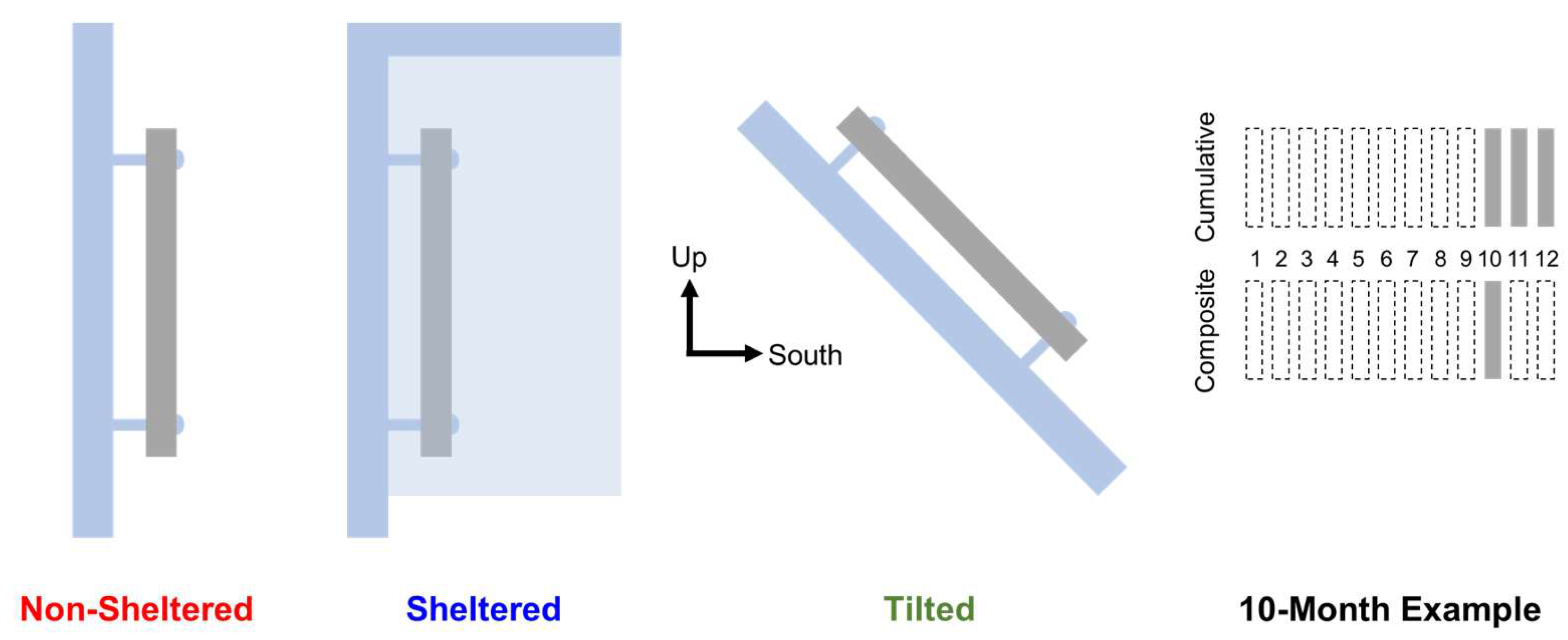
• The way in which a sample is exposed for atmospheric testing greatly influences the resulting corrosion damage. A Tilted condition was found to be more aggressive than vertical conditions in which a sample was either Sheltered or Non-Sheltered (Figure 5). This was attributed to a greater propensity for sea spray aerosol salt deposition flux and solar irradiance (Southward facing samples).
• Smaller samples of C1010 steel had greater mass loss density values (g/m²) than larger steel samples despite correcting for the difference in the surface area. The Thin samples had about 15–45% greater mass loss than the Wide samples (Figure 5). This discrepancy was attributed to an edge effect where the edge is more susceptible to corrosion attack. Such an edge effect would be more pronounced for smaller samples. It is unclear why the Tilted samples had a smaller difference between the Wide and Thin geometries than the other conditions.
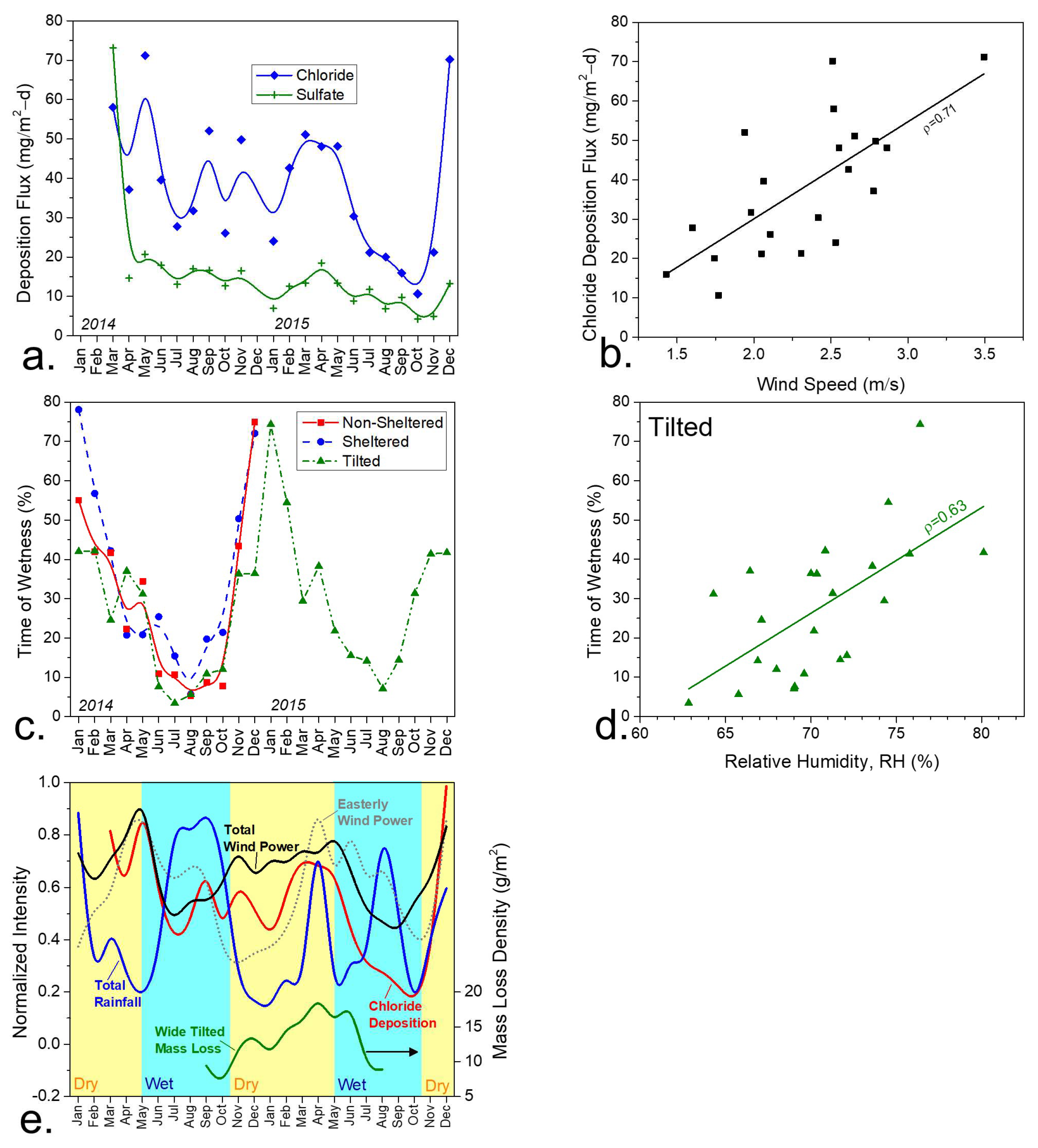
• Easterly wind power, specifically, was found to be strongly controlling in the Key West-exposed C1010 mass loss (Figure 10). Steel mass loss was greatest for Key West in April and least in October (Figure 7). The mass loss was found to be generally higher during the dry season (in terms of precipitation) when the time of wetness is highest. The mass loss was the highest during the transition from the dry season to the wet season (Figure 8).
• Short term exposures yielded mass loss rates that are greater than those rates determined from longer-term exposure. This was attributed to the development of a thick corrosion scale that mediates corrosion processes. For this reason, the additive composite mass loss of multiple months stitched together overestimates what the mass loss values are for cumulative samples exposed for the equivalent length of time (Figure 6). This highlights the importance of long-term corrosion testing.
• In all, corrosion damage assessment was greatly influenced by the details of the exposure design. Tilt, sheltering, sample size, exposure start, and exposure duration were all controlling factors. The importance of reducing the variability in field exposure studies in atmospheric corrosion is underscored.

References

- Ambler, H.R.; Bain, A.A.J. Corrosion of Metals in the Tropics. J. Appl. Chem. 1955, 5, 437–467. [Google Scholar] [CrossRef]
- Cole, I.S.; Muster, T.H.; Azmat, N.S.; Venkatraman, M.S.; Cook, A. Multiscale Modelling of the Corrosion of Metals under Atmospheric Corrosion. Electrochim. Acta 2011, 56, 1856–1865. [Google Scholar] [CrossRef]
- Leygraf, C.; Wallinder, I.O.; Tidblad, J.; Graedel, T. Atmospheric Corrosion; The Ecs Series of Texts and Monographs; Wiley: Hoboken, NJ, USA, 2016. [Google Scholar]
- Li, S.; Hihara, L.H. Aerosol Salt Particle Deposition on Metals Exposed to Marine Environments: A Study Related to Marine Atmospheric Corrosion. J. Electrochem. Soc. 2014, 161, C268–C275. [Google Scholar] [CrossRef]
- Schindelholz, E.; Risteen, B.; Kelly, R.G. Atmospheric Corrosion of Plain Carbon Steel Below the Deliquescence Point of Sodium Chloride. In Meeting Abstracts; The Electrochemical Society, Inc.: Pennington, NJ, USA, 2013; p. 1735. [Google Scholar]
- Tomashov, N.D. Development of the Electrochemical Theory of Metallic Corrosion. Corrosion 2013, 20, 7t–14t. [Google Scholar] [CrossRef]
- Cook, A.B.; Lyon, S.B.; Stevens, N.P.C.; Gunther, M.; McFiggans, G.; Newman, R.C.; Engelberg, D.L. Assessing the Risk of under-Deposit Chloride-Induced Stress Corrosion Cracking in Austenitic Stainless Steel Nuclear Waste Containers. Corros. Eng. Sci. Technol. 2014, 49, 529–534. [Google Scholar] [CrossRef]
- Liang, D.; Allen, H.C.; Frankel, G.S.; Chen, Z.Y.; Kelly, R.G.; Wu, Y.; Wyslouzil, B.E. Effects of Sodium Chloride Particles, Ozone, Uv, and Relative Humidity on Atmospheric Corrosion of Silver. J. Electrochem. Soc. 2010, 157, C146–C156. [Google Scholar] [CrossRef]
- Meira, G.R.; Andrade, C.; Alonso, C.; Padaratz, I.J.; Borba, J.C. Modelling Sea-Salt Transport and Deposition in Marine Atmosphere Zone—A Tool for Corrosion Studies. Corros. Sci. 2008, 50, 2724–2731. [Google Scholar] [CrossRef]
- Morcillo, M.; Chico, B.; Mariaca, L.; Otero, E. Salinity in Marine Atmospheric Corrosion: Its Dependence on the Wind Regime Existing in the Site. Corros. Sci. 2000, 42, 91–104. [Google Scholar] [CrossRef]
- Schindelholz, E.; Robert, G.K. Wetting Phenomena and Time of Wetness in Atmospheric Corrosion: A Review. Corros. Rev. 2012, 30, 135–170. [Google Scholar] [CrossRef]
- Schindelholz, E.; Risteen, B.E.; Kelly, R.G. Effect of Relative Humidity on Corrosion of Steel under Sea Salt Aerosol Proxies. J. Electrochem. Soc. 2014, 161, C460–C470. [Google Scholar] [CrossRef]
- Tiwari, S.; Hihara, L.H. Development of a Corrosion Model to Correlate the Atmospheric Corrosion Rate of a Carbon-Fiber Reinforced Aluminum Mmc to Weather and Environmental Parameters. J. Electrochem. Soc. 2014, 161, C382–C388. [Google Scholar] [CrossRef]
- Cheng, Y.L.; Zhang, Z.; Cao, F.H.; Li, J.F.; Zhang, J.Q.; Wang, J.M.; Cao, C.N. A Study of the Corrosion of Aluminum Alloy 2024-T3 under Thin Electrolyte Layers. Corros. Sci. 2004, 46, 1649–1667. [Google Scholar] [CrossRef]
- Rafla, V.N.; Khullar, P.; Kelly, R.G.; Scully, J.R. Coupled Multi-Electrode Array with a Sintered Ag/Agcl Counter/Reference Electrode to Investigate Aa7050-T7451 and Type 316 Stainless Steel Galvanic Couple under Atmospheric Conditions. J. Electrochem. Soc. 2018, 165, C562–C572. [Google Scholar] [CrossRef]
- Schindelholz, E.J.; Cong, H.; Jove-Colon, C.F.; Li, S.; Ohlhausen, J.A.; Moffat, H.K. Electrochemical Aspects of Copper Atmospheric Corrosion in the Presence of Sodium Chloride. Electrochim. Acta 2018, 276, 194–206. [Google Scholar] [CrossRef]
- Shedd, M. Modeling and Measurement of the Maximum Pit Size on Ferrous Alloys Exposed to Atmospheric Conditions. Master’s Thesis, University of Virginia, Charlottesville, VA, USA, 2012. [Google Scholar]
- Tereshchenko, A.G. Deliquescence: Hygroscopicity of Water-Soluble Crystalline Solids. J. Pharm. Sci. 2015, 104, 3639–3652. [Google Scholar] [CrossRef] [PubMed]
- King, A.D.; Lee, J.S.; Scully, J.R. Finite Element Analysis of the Galvanic Couple Current and Potential Distribution between Mg and 2024-T351 in a Mg Rich Primer Configuration. J. Electrochem. Soc. 2016, 163, C342–C356. [Google Scholar] [CrossRef]
- Prosek, T.; Iversen, A.; Taxén, C.; Thierry, D. Low-Temperature Stress Corrosion Cracking of Stainless Steels in the Atmosphere in the Presence of Chloride Deposits. Corrosion 2009, 65, 105–117. [Google Scholar] [CrossRef]
- Fitzgerald, J.W. Marine Aerosols: A Review. Atmos. Environ. Part A. Gen. Top. 1991, 25, 533–545. [Google Scholar] [CrossRef]
- Meira, G.R.; Andrade, C.; Alonso, C.; Padaratz, I.J.; Borba, J.C. Salinity of Marine Aerosols in a Brazilian Coastal Area—Influence of Wind Regime. Atmos. Environ. 2007, 41, 8431–8441. [Google Scholar] [CrossRef]
- Meira, G.R.; Andrade, M.C.; Padaratz, I.J.; Alonso, M.C.; Borba, J.C., Jr. Measurements and Modelling of Marine Salt Transportation and Deposition in a Tropical Region in Brazil. Atmos. Environ. 2006, 40, 5596–5607. [Google Scholar] [CrossRef]
- Pham, N.D.; Kuriyama, Y.; Kasai, N.; Okazaki, S.; Suzuki, K.; Nguyen, D.T. A New Analysis of Wind on Chloride Deposition for Long-Term Aerosol Chloride Deposition Monitoring with Weekly Sampling Frequency. Atmos. Environ. 2019, 198, 46–54. [Google Scholar] [CrossRef]
- Standard Guide for Conducting Corrosion Tests in Field Applications; ASTM International: West Conshohocken, PA, USA, 2014.
- Standard Practice for Conducting Atmospheric Corrosion Tests on Metals; ASTM International: West Conshohocken, PA, USA, 2015.
- ISO. Classification, Determination and Estimation. In Corrosion of Metals and Alloys—Corrosivity of Atmospheres, 15; International Organization for Standardization: Geneva, Switzerland, 2012. [Google Scholar]
- Guiding Values for the Corrosivity Categories. In Corrosion of Metals and Alloys—Corrosivity of Atmospheres; International Organization for Standardization: Geneva, Switzerland, 2012.
- Measurement of Environmental Parameters Affecting Corrosivity of Atmospheres. In Corrosion of Metals and Alloys—Corrosivity of Atmospheres; International Organization for Standardization: Geneva, Switzerland, 2012.
- Schindelholz, E.; Kelly, R.G.; Cole, I.S.; Ganther, W.D.; Muster, T.H. Comparability and Accuracy of Time of Wetness Sensing Methods Relevant for Atmospheric Corrosion. Corros. Sci. 2013, 67, 233–241. [Google Scholar] [CrossRef]
- ASTM International. Standard Test Method for Determining Atmospheric Chloride Deposition Rate by Wet Candle Method; American Society for Testing and Materials International: West Conshohocken, PA, USA, 2014. [Google Scholar]
- Santucci, R.J., Jr.; Davis, R.; Sanders, C. Precision of the Wet Candle for Chloride Analysis; Open Science Framework, Ed.; Open Science Framework: Charlottesville, VA, USA, 2021. [Google Scholar]
- Santucci, R.J.; Davis, R.S.; Sanders, C.E. Atmospheric Corrosion Severity and the Precision of Salt Deposition Measurements Made by the Wet Candle Method. Corros. Eng. Sci. Technol. 2021, 57, 147–158. [Google Scholar] [CrossRef]
- Ann, K.Y.; Song, H.-W. Chloride Threshold Level for Corrosion of Steel in Concrete. Corros. Sci. 2007, 49, 4113–4133. [Google Scholar] [CrossRef]
- Chen, Z.Y.; Zakipour, S.; Persson, D.; Leygraf, C. Effect of Sodium Chloride Particles on the Atmospheric Corrosion of Pure Copper. Corrosion 2004, 60, 479–491. [Google Scholar] [CrossRef]
- Xie, Y.; Zhang, J. Chloride-Induced Stress Corrosion Cracking of Used Nuclear Fuel Welded Stainless Steel Canisters: A Review. J. Nucl. Mater. 2015, 466, 85–93. [Google Scholar] [CrossRef]
- Cole, I.S.; Ganther, W.D.; Paterson, D.A.; King, G.A.; Furman, S.A.; Lau, D. Holistic Model for Atmospheric Corrosion: Part 2—Experimental Measurement of Deposition of Marine Salts in a Number of Long Range Studies. Corros. Eng. Sci. Technol. 2003, 38, 259–266. [Google Scholar] [CrossRef]
- Meyers, T.P.; Finkelstein, P.; Clarke, J.; Ellestad, T.G.; Sims, P.F. A Multilayer Model for Inferring Dry Deposition Using Standard Meteorological Measurements. J. Geophys. Res. Atmos. 1998, 103, 22645–22661. [Google Scholar] [CrossRef]
- Petroff, A.; Zhang, L. Development and Validation of a Size-Resolved Particle Dry Deposition Scheme for Application in Aerosol Transport Models. Geosci. Model Dev. 2010, 3, 753–769. [Google Scholar] [CrossRef]
- Schindelholz, E. Towards Understanding Surface Wetness and Corrosion Response of Mild Steel in Marine Atmospheres. Ph.D. Thesis, University of Virginia, Charlottesville, VA, USA, 2014. [Google Scholar]
- Peel, M.C.; Finlayson, B.L.; McMahon, T.A. Updated World Map of the Köppen-Geiger Climate Classification. Hydrol. Earth Syst. Sci. 2007, 11, 1633–1644. [Google Scholar] [CrossRef]
- Meira, G.R.; Andrade, C.; Padaratz, I.J.; Alonso, C.; Borba, J.C., Jr. Chloride Penetration into Concrete Structures in the Marine Atmosphere Zone—Relationship between Deposition of Chlorides on the Wet Candle and Chlorides Accumulated into Concrete. Cem. Concr. Compos. 2007, 29, 667–676. [Google Scholar] [CrossRef]
- McMahon, M.E.; Santucci, R.J.; Scully, J.R. Advanced Chemical Stability Diagrams to Predict the Formation of Complex Zinc Compounds in a Chloride Environment. RSC Adv. 2019, 9, 19905–19916. [Google Scholar] [CrossRef] [PubMed]
- Abbott, W.H. A Decade of Corrosion Monitoring in the World’s Military Operating Environments: A Summary of Results; Battelle Columbus Operations: Columbus, OH, USA, 2008. [Google Scholar]