1. Introduction
Picture a historical building as an enigmatic puzzle, each crack, deformation, and hidden corrosion forming the cryptic pieces waiting to be deciphered. As we stand at the intersection of technology and architectural history, our pursuit is to decode this intricate puzzle. Multisensor data fusion emerges as our toolkit, seamlessly blending the precision of laser scanners with the spectral insight of photographic cameras. Here, we introduce a revolutionary approach, not just to study buildings, but to unravel the mysteries concealed within their weathered walls.
The state-of-the-art in multisensor data fusion in the study of building pathologies has undergone significant advances in the last decades. The convergence of various technologies and sensors has enabled researchers to assess structural conditions and pathologies in buildings more fully and accurately [
1,
2].
Studies on potential issues in historical buildings employing geomatic sensor technology have garnered diverse attention in late years [
3,
4]. First approaches were dedicated only to generate three-dimensional models with different levels of detail. These three-dimensional models were complemented by spectral information so that visual representations could be made to highlight areas that could present some pathology [
5,
6].
Various studies have focused on different architectural elements and their specific pathologies. For example, in the study of façades [
7,
8,
9] or concrete structural elements [
10,
11,
12]. The data obtained were sometimes integrated into Building Information Models (BIM) for further study [
13,
14].
In turn, different research works have concentrated on the use of singular sensors. There are research works focused on the use of infrared thermal cameras [
15,
16,
17,
18,
19], multispectral photographic cameras [
20,
21] and laser scanners [
22,
23,
24].
The combined use of active and passive sensors such as terrestrial laser scanners and photographic cameras with different spectral sensitivities has provided a wealth of information. This allows the generation of detailed three-dimensional models, point clouds with spectral information, and visual representations highlighting the affected areas. This combination of different sensor types provides a complete view of the structure and its potential pathologies. Terrestrial laser scanners capture highly detailed three-dimensional point clouds, thereby facilitating the detection of structural deformations and cracks [
25,
26]. Photographic cameras provide valuable spectral information that can indicate signs of corrosion, moisture, or other problems that can not be visible to the naked eye.
The use of 3D point clouds requires the management of an immense volume of data, which requires substantial data-processing infrastructure for handling and visualization. Additionally, 3D point clouds are inherently unstructured, making the task of locating specific points within these clouds nontrivial [
27]. One consequence of this lack of structure is that point clouds do not contain topological information, thereby precluding an understanding of neighborhood relationships among points [
28].
Point clouds also exhibit non-uniform densities and distributions. The point density achieved is not always optimal for the intended applications. Some areas will display redundant information, particularly in the overlapping zones between scans. Conversely, other areas will present lower point densities. This results in heterogeneity in both the density and accuracy of points within the cloud [
29].
In terms of analysis, multisensor data fusion has enabled the early detection and monitoring of structural pathologies, such as cracks, deformations, and corrosion. In addition, the integration of information from airborne and ground sensors has enabled more complete coverage of structures, both in terms of physical access and data diversity. Traditionally, the assessment of structural problems involves visual inspections, manual measurements, and, at best, the use of a single sensor to capture limited data [
30]. Modern data fusion systems allow the creation of accurate three-dimensional digital models that can be compared to the original designs to identify discrepancies. This is especially valuable for assessing the performance of historic structures and monuments where preservation is critical [
31].
The integration of various sensors and techniques also leads to the creation of diverse point cloud datasets, which in turn contributes to the formation of large data repositories [
29]. This not only affects processing speed but also requires the conversion of substantial volumes of point data into dependable and actionable insights. Traditional methods for customizing point clouds for specific applications are becoming increasingly time consuming and require manual intervention. The growing complexity and volume of data, often spread across multiple stakeholders or platforms, pose a challenge to human expertise in effective data management [
32]. To facilitate more effective decision making, it is crucial to efficiently convert voluminous point cloud data into streamlined processes, thereby heralding a new age of decision-support services. Strategies must be developed for extensive automation and structuring to eliminate the need for task-specific manual processing and to promote sustainable collaboration.
Voxels have been used in a variety of distinct fields, including geology [
33], forest inventory [
34], and medical research [
35]. In the context of their application to point cloud management, multiple studies [
36,
37,
38,
39,
40] have substantiated the efficacy of voxels as an appropriate tool for handling point cloud data.
Voxelization is more beneficial for managing raw 3D point clouds. With the points being placed in a regular grid pattern, it is now possible to structure the point cloud in a tree format that allows for significantly reduced computing time. Logical inference is also possible from a voxel structure because the known relationship with neighboring points allows for semantic reasoning [
41].
In voxelization of point clouds, one defining parameter of the voxel structure is the elemental voxel size. This parameter governs the resolution of the phenomena under study through the data structure, impacting various applications, such as finite elements [
42], structural analyses [
43,
44], and dynamic phenomena [
45]. For instance, if a study or simulation requires a resolution of 5 cm, this would dictate the voxel elemental size established during the voxelization process. In addition, voxel size determines the extent of element reduction relative to the number of points present in the original clouds [
29].
The application of deep learning algorithms to voxel structures is an active research area across various fields, such as computer vision, robotics, geography, and medicine. Within the spectrum of deep learning approaches applied to voxels, some notable methodologies as 3D Convolutional Neural Networks (3D CNNs) [
46,
47], Voxel-based Autoencoders [
48,
49], Generative Networks for Voxels [
50,
51,
52], and Semantic Segmentation [
28,
53] have been used.
However, despite these advances, challenges still exist in terms of accurate calibration, data correction, and effective integration of the collected information. Additionally, the interpretation of merged data requires expertise in remote sensing and structural analysis to avoid false diagnoses. Accurate integration of data from different sources requires careful calibration and correction [
54]. In addition, proper interpretation of results remains crucial, as the presence of detailed data does not always guarantee a complete understanding of the underlying causes of pathologies.
In this paper, we present a novel approach to multisensor data fusion using multispectral voxels. This data fusion allows for optimal and efficient management of the sensors information, allowing later applications of deep learning algorithms. With this, a workflow is determined that allows the study of buildings as well as the possible pathologies that could be present on them.
This study is organized as follows. Initially, the sensors that were used in a data acquisition campaign on a prominent Spanish Cultural Heritage building are described. Subsequently, the methodology that was designed for handling, processing, and fusing the data using our concept of multispectral voxels is outlined. The deep learning Self-organizing map algorithm will be applied to our multispectral voxel structure. Finally, we discuss the results.
2. Materials and Methods
2.1. Sensors
Within the context of multisensor fusion, a data-capture campaign with a range of different sensors featuring distinct spectral sensitivities and types were chosen. To this end, active and passive sensors were used. The set of active sensors comprises terrestrial laser scanners, whereas the passive sensor group encompasses a variety of photographic cameras deployed in both terrestrial and aerial arrangements using Unmanned Aerial Vehicles (UAVs). Each camera had distinct spectral sensitivities.
This meticulous selection of sensors encompasses various conventional modalities of geospatial data capture, which are commonly employed in the analysis of buildings and architectural structures. The acquired data were subjected to a series of processing techniques, with photogrammetry as one of the principal methodologies. Consequently, the final output consisted of multiple point cloud datasets, each characterized by unique and significant spectral properties.
While developing the data capture strategy, it was acknowledged that not all sensors were capable of capturing data encompassing the entire built structure. Sensors located on the ground can only provide information about the lower sections of the building, while sensors attached to aerial vehicles can capture data covering the entire architectural unit. This distinction is essential for accurate interpretation and cohesive integration of the collected data during the analytical process.
The employed sensors are described herein, including photographic cameras, unmanned aerial sensors (UAVs), and laser scanners:
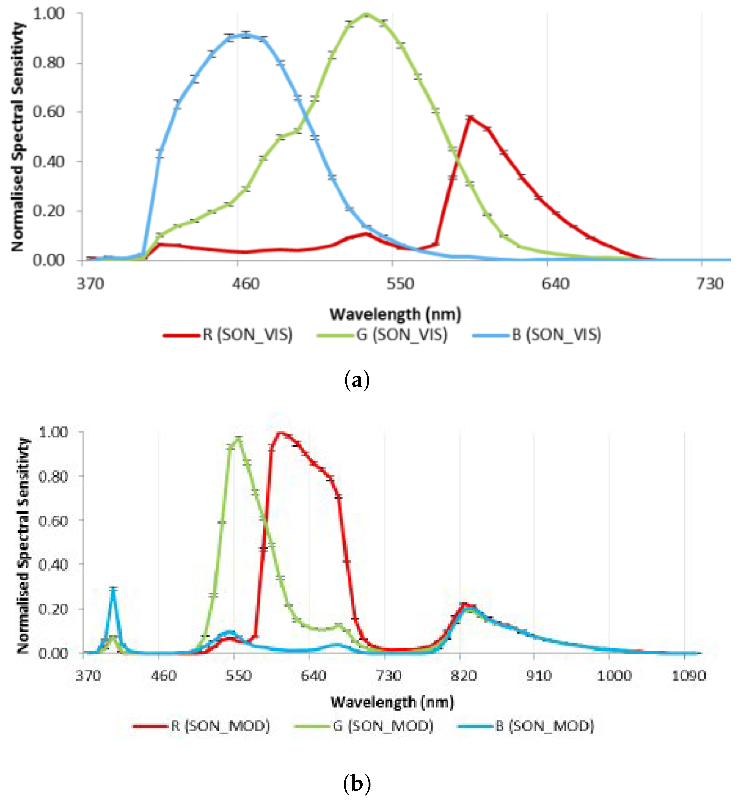
The terrestrial digital imaging device deployed was a Sony NEX-7 photographic camera (Sony Corporation, Tokyo, Japan), a model equipped with a 19 mm optical lens of fixed length. This particular sensor captures spectral components within the red (590 nm), green (520 nm), and blue (460 nm) bands of the visible spectrum. The spectral response of this camera is illustrated in
Figure 1a, and its specific parameters are outlined in
Table 1.
Table 1.
Sony NEX 7 camera sensor parameters.
Table 1.
Sony NEX 7 camera sensor parameters.
| Parameter | Value |
|---|
| Sensor | APS-C type CMOS sensor |
| Focal lenght (mm) | 19 |
| Sensor width (mm) | 23.5 |
| Sensor lenght (mm) | 15.6 |
| Effective pixels (megapixels) | 24.3 |
| Pixel size (micrometers) | 3.92 |
| ISO sensitivity range | 100–1600 |
| Image format | RAW (Sony ARW 2.3 format) |
| Weight (g) | 350 |
A modified version of the digital image camera, the Sony NEX-5N model, was also employed in terrestrial positions. It was outfitted with a 16 mm fixed-length lens, accompanied by a near-infrared (NIR) filter and an ultraviolet (UV) filter in different shot sessions. Detailed information on this sensor is provided in
Table 2.
Table 2.
Sony NEX 5N camera sensor parameters.
Table 2.
Sony NEX 5N camera sensor parameters.
| Parameter | Value |
|---|
| Sensor | APS-C type CMOS sensor |
| Focal lenght (mm) | 16 |
| Sensor width (mm) | 23.5 |
| Sensor lenght (mm) | 15.6 |
| Effective pixels (megapixels) | 16.7 |
| Pixel size (micrometers) | 4.82 |
| ISO sensitivity range | 100–3200 |
| Image format | RAW (Sony ARW 2.2 format) |
| Weight (g) | 269 |
By removing the internal infrared filter from the Sony NEX-5N camera, the sensitivity of the sensor was enhanced to encompass specific regions of the electromagnetic spectrum, including the near-infrared (820 nm) and ultraviolet (390 nm) wavelengths. The spectral responsiveness of this modified camera is shown in
Figure 1b. Notably, the modified sensor exhibits sensitivity to distinct segments of the electromagnetic spectrum in contrast to its unmodified counterpart, the Sony NEX-7, which retains the internal infrared filter (as illustrated in
Figure 1a) [
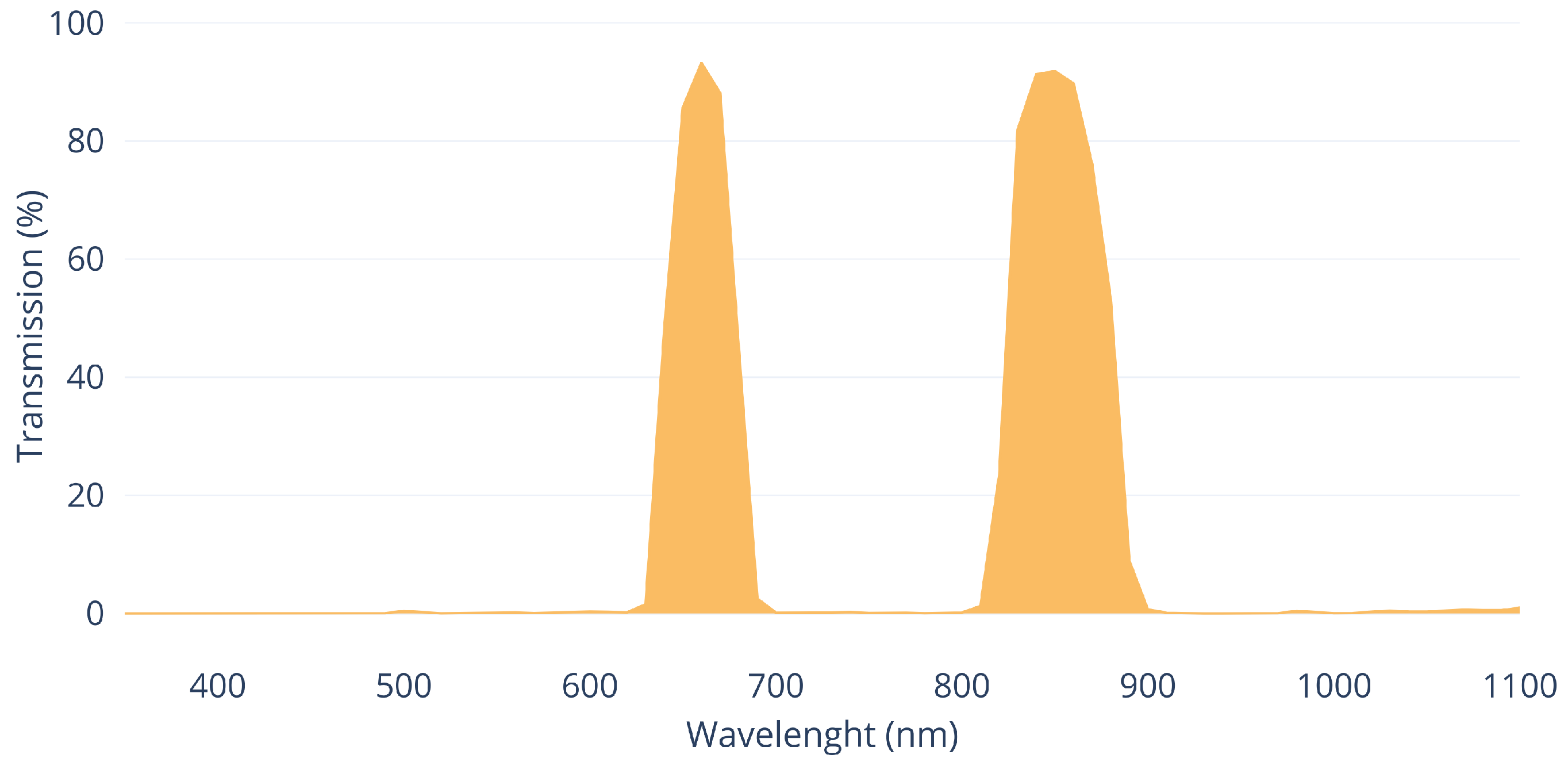
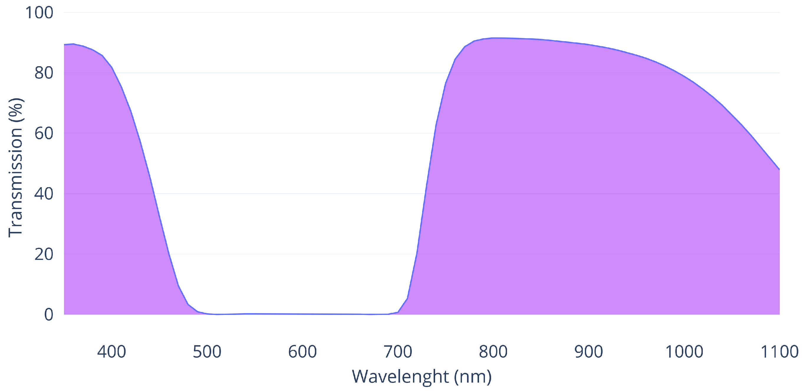
55]. This modified camera was equipped with a collection of filters to obtain data corresponding to ultraviolet (UV) and near-infrared (NIR) spectral bands. The transmission curves of the filters employed during the data acquisition process are shown in
Figure 2 and
Figure 3.
The terrestrial laser scanner employed in this study was the Faro Focus S350 laser scanner, developed by Faro Technologies (Lake Mary, FL, USA). It has proven to be an invaluable tool for archaeological and building studies applications. Its cutting-edge phase-based laser scanning technology enables it to accurately measure distances and efficiently gather an extensive dataset of millions of data points in a short span. Particularly relevant in archaeological studies, this scanner aids in documenting historical sites and structures with high precision. The Faro Focus S350 laser beam wavelength is 1550 nm (
Table 3). This allowed us to obtain building spectral information in the short-wavelength infrared spectral (SWIR) band [
56]. Concerning the use of data derived from the laser scanner, the registered return signal intensity value has been used as its application has been demonstrated to be effective in buildings made of stone [
22].
Figure 1.
Spectral responses for Sony NEX cameras, from [
55]: (
a) Unmodified camera, normalized to the peak of the green channel. (
b) Modified camera, normalized to the peak of the red channel.
Figure 1.
Spectral responses for Sony NEX cameras, from [
55]: (
a) Unmodified camera, normalized to the peak of the green channel. (
b) Modified camera, normalized to the peak of the red channel.
Figure 2.
Midopt DB 660/850 Dual Bandpass filter light transmission curve (Midwest Optical Systems, Inc., Palatine, IL, USA).
Figure 2.
Midopt DB 660/850 Dual Bandpass filter light transmission curve (Midwest Optical Systems, Inc., Palatine, IL, USA).
Figure 3.
ZB2 filter light transmission curve, from Shijiazhuang Tangsinuo Optoelectronic Technology Co., Ltd., Shijiazhuang, Hebei, China.
Figure 3.
ZB2 filter light transmission curve, from Shijiazhuang Tangsinuo Optoelectronic Technology Co., Ltd., Shijiazhuang, Hebei, China.
For data collection in the upper regions of the building, where ground-based sensors lack access, an Unmanned Aerial Vehicle (UAV) was deployed. The chosen instrument was the Parrot Anafi Thermal (
Table 4), which mounts a dual-camera system comprising an RGB sensor (for the visible spectrum) and an infrared thermal sensor. This configuration facilitates the simultaneous capture of conventional RGB and infrared thermal images within a single flight mission. Referring to the thermal infrared data, the Parrot Anafi Thermal incorporates a factory-calibrated uncooled microbolometer-type FLIR Lepton 3.5 thermal module [
57], enabling the establishment of an absolute temperature for each image pixel. Consequently, precise surface temperatures of the building points were determined. This aids in discerning the discontinuities and potential pathologies resulting from the heterogeneity of construction materials [
19].
2.2. Data Capture Campaign
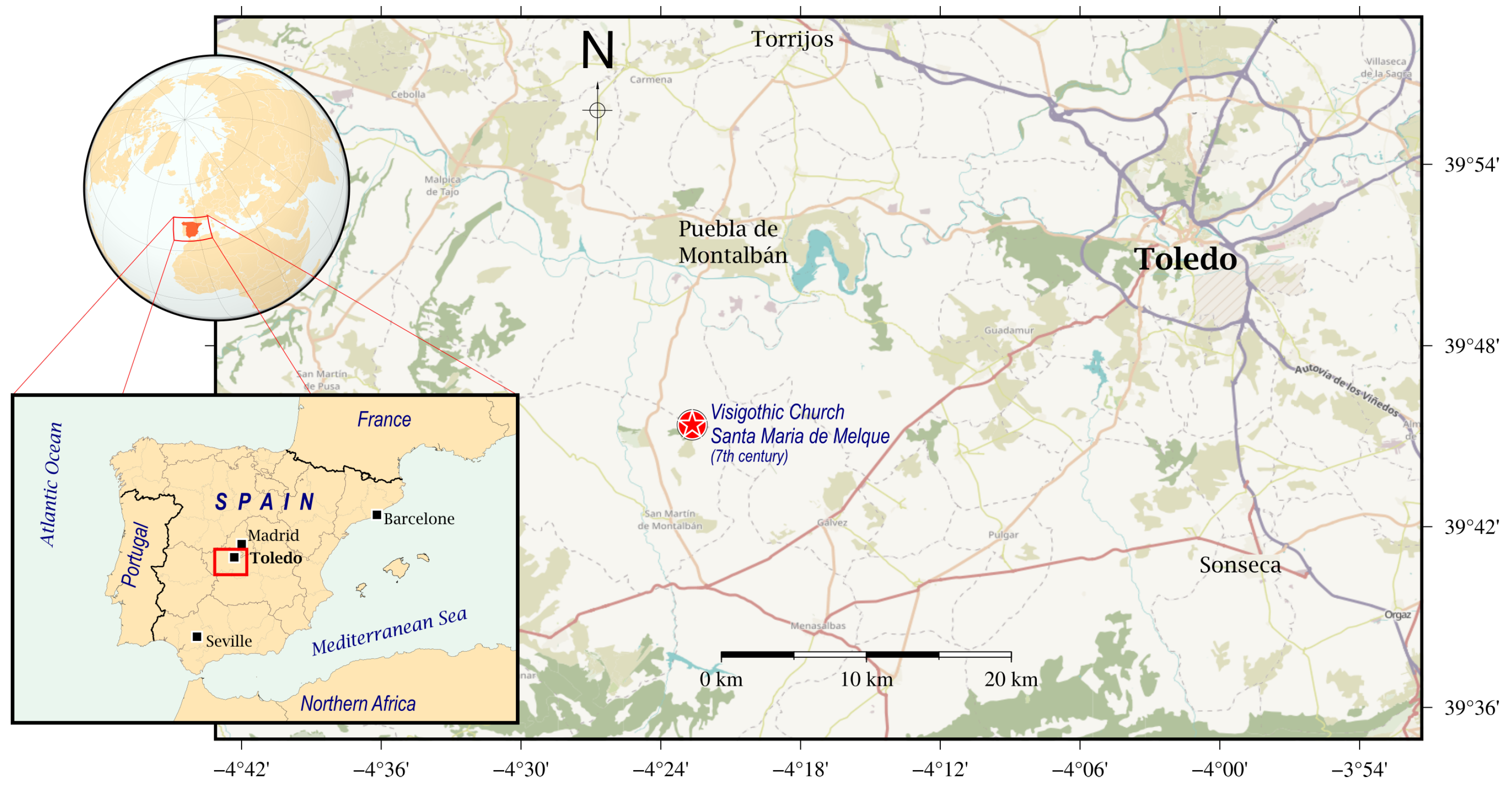
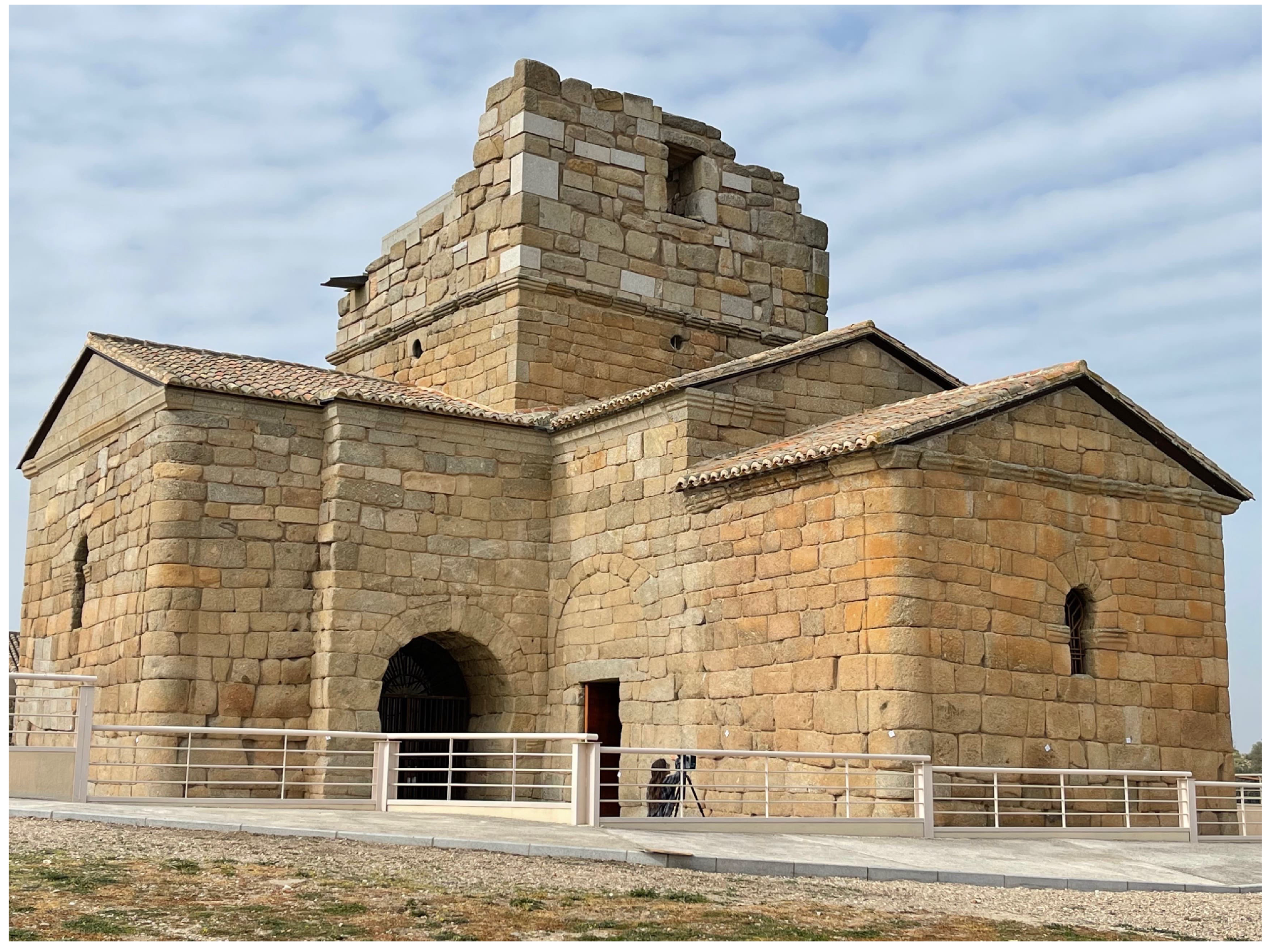
For data acquisition, an emblematic building of Spanish historical heritage was selected. The chosen structure was the Visigothic Church of the Santa Maria de Melque. Data from all the described sensors were directly collected on this 7th-century A.D. building [
58], located in the province of Toledo, Spain. The archaeological complex of Santa Maria de Melque (N 39.750878°, W 4.372965°) is located approximately 30 km southwest of the city of Toledo, in close proximity to the Tagus River [
59] (
Figure 4).
The structure of the Visigothic church of Santa Maria de Melque was constructed using masonry of immense granite blocks assembled without mortar, distinguished by its barrel vault covering the central nave. The layout of the aisles in the form of a Greek cross, the straight apse, and the arrangement of architectural elements reveal both Roman and Byzantine influences, reflecting the rich cultural diversity of the period [
60].
The data collection campaign was carried out only on the exterior of this building in February 2022. The campaign covered the entire architectural structure and its ornamental elements. This location was chosen for its historical and architectural relevance, which allowed us to obtain precise and detailed information on the current state of the building and its possible pathologies.
Figure 5 shows the studied building.
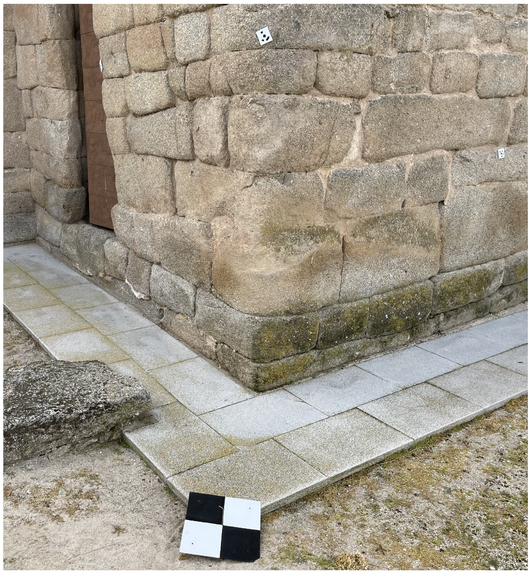
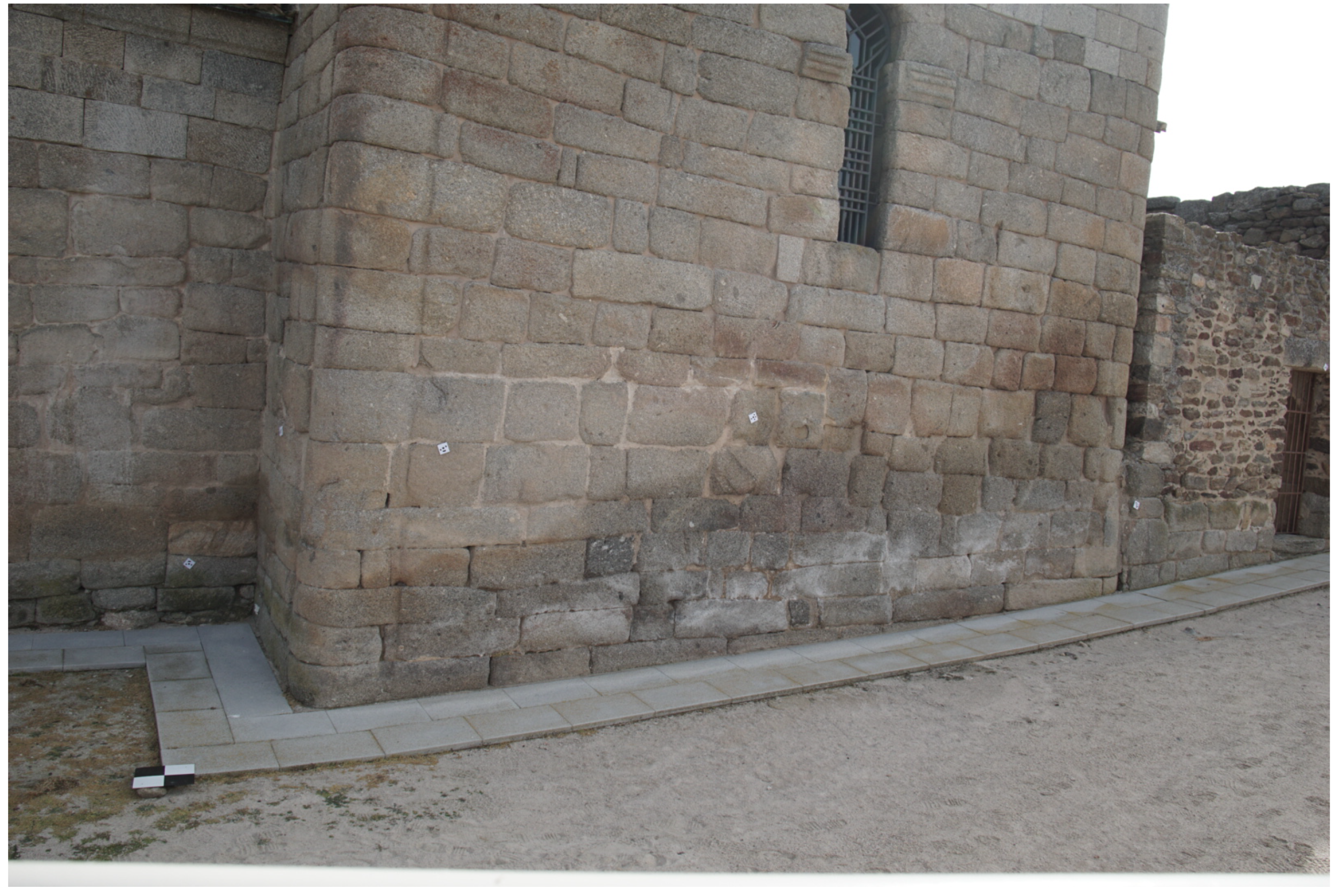
Prior to capturing the dataset, a meticulous preparatory phase was undertaken, involving the careful placement of a series of precision targets across the walls surface. These identified markers collectively formed a robust set of control points that served as pivotal anchors for the subsequent data collection process. By ensuring uniformity and accuracy at these measurement points, a reliable common geometric reference system was established, effectively standardizing the subsequent data acquisition process across all data collection sessions. This rigorous methodology not only underscored the accuracy of the data collected but also facilitated seamless comparability and analysis of the collected visual information (
Figure 6).
The Terrain Target Signals (TTS) were measured using GNSS techniques. These marks were materialized by means of a metal nail in the ground, in order to be revisited on future occasions. Subsequently, a flat black-and-white square sign measuring 30 cm on each side was adopted (
Figure 6).
For the observation, dual-frequency Topcon Hiper GNSS receivers were used, with calibrated antennas (GPS, GLONASS), tripod and centering system on the point mark, measuring a total of 12 TTS, forming a network of 30 vectors. The observation time at each point was 15–20 min, with at least a double observation session at each point with different receivers, thus configured in relative static surveying with high repeatability.
In the subsequent processing of GNSS data, to obtain greater precision in the results, the precise geodetic correction models of the ionosphere from the CODE (Center for Orbit Determination in Europe) and precise ephemeris from the IGS (International GNSS Service) for both constellations were downloaded. Along with these Topcon field GNSS data, data from continuous CORS (Continuously Operating Reference Stations) of the Spanish National Positioning System ERGNSS-IGN (Instituto Geográfico Nacional) were also processed. This was done in order to link the local GNSS measurements to a geodetic reference frame that guaranteed high precision stability and temporal permanence for future actions in the environment.
To compute the GNSS vectors, the Leica Infinity version 3.0.1 software was used, using the absolute antenna calibration models and using the VMF (Vienna Mapping Functions) [
61]. Both for the observation and for the adjustment and compensation of the coordinates of all the TTS points that make up the network, the same methodology used in the implementation of geodetic precision control networks in engineering was followed [
62]. The final adjustment of the network, the calculation of the coordinates and the estimation of its accuracy (
Table 5) was performed with Geolab version px5 software, with a complete constraint in the ETRS89 (ETRF2000) frame.
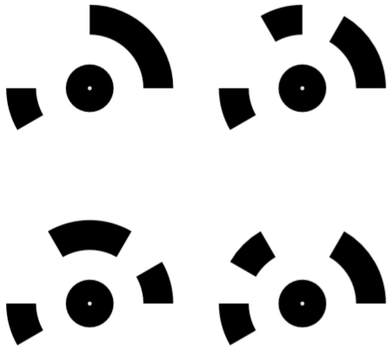
Wall Surface Signals (WSS) were placed around the entire building and attached to the wall. They are intended to tie points supporting the georeferencing process in all point clouds. WSS were 12 bit coded precision targets (
Figure 7). Thus, each WSS can be clearly identified by photogrammetry software, almost in automatic mode, and operators.
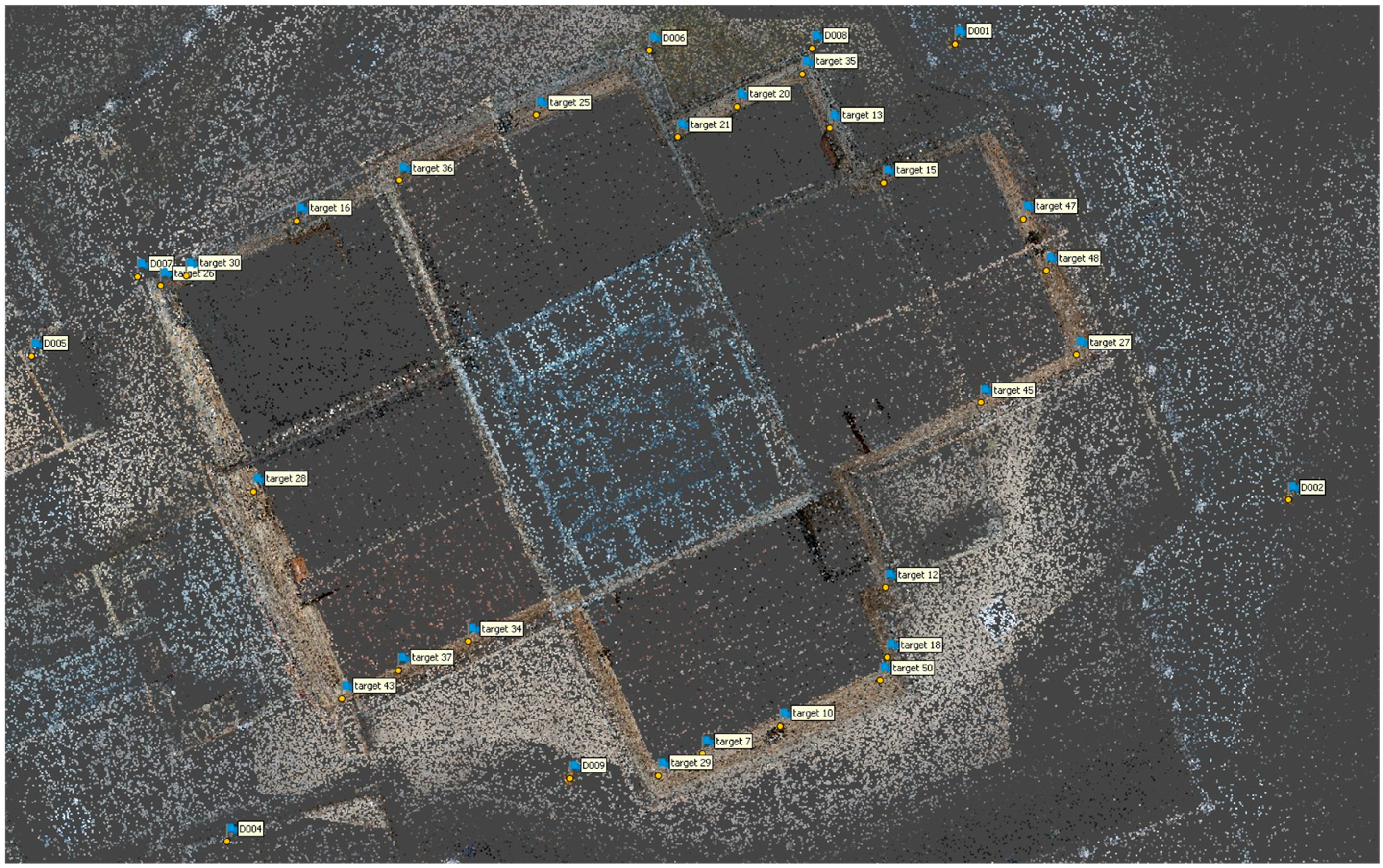
In
Figure 8, we show the distribution of targets on terrain (TTS) and on the walls (WSS). The coordinates of the precision targets attached to the walls (Wall Surface Signals) are expressed in
Table A1.
2.3. Point Clouds
In the course of this research, a range of sensors were used for the collection of geomatic data across multiple spectral bands. The processing of each dataset has been carried out with great care, resulting in the generation of several georreferenced three-dimensional point clouds. These point clouds offer a comprehensive and diverse view of the building under examination from various angles (as presented in
Table 6). Each point cloud, except the laser scanner point cloud, comes from a photogrammetric process. The photogrammetric software used was Agisoft Metashape version 1.8.5. All derived photogrammetry point clouds are the result of processing a single sensor in a single process. Only in RGB point cloud, unmodified terrestrial RGB camera and UAV RGB image datasets were combined in the same process to obtain the RGB point cloud.
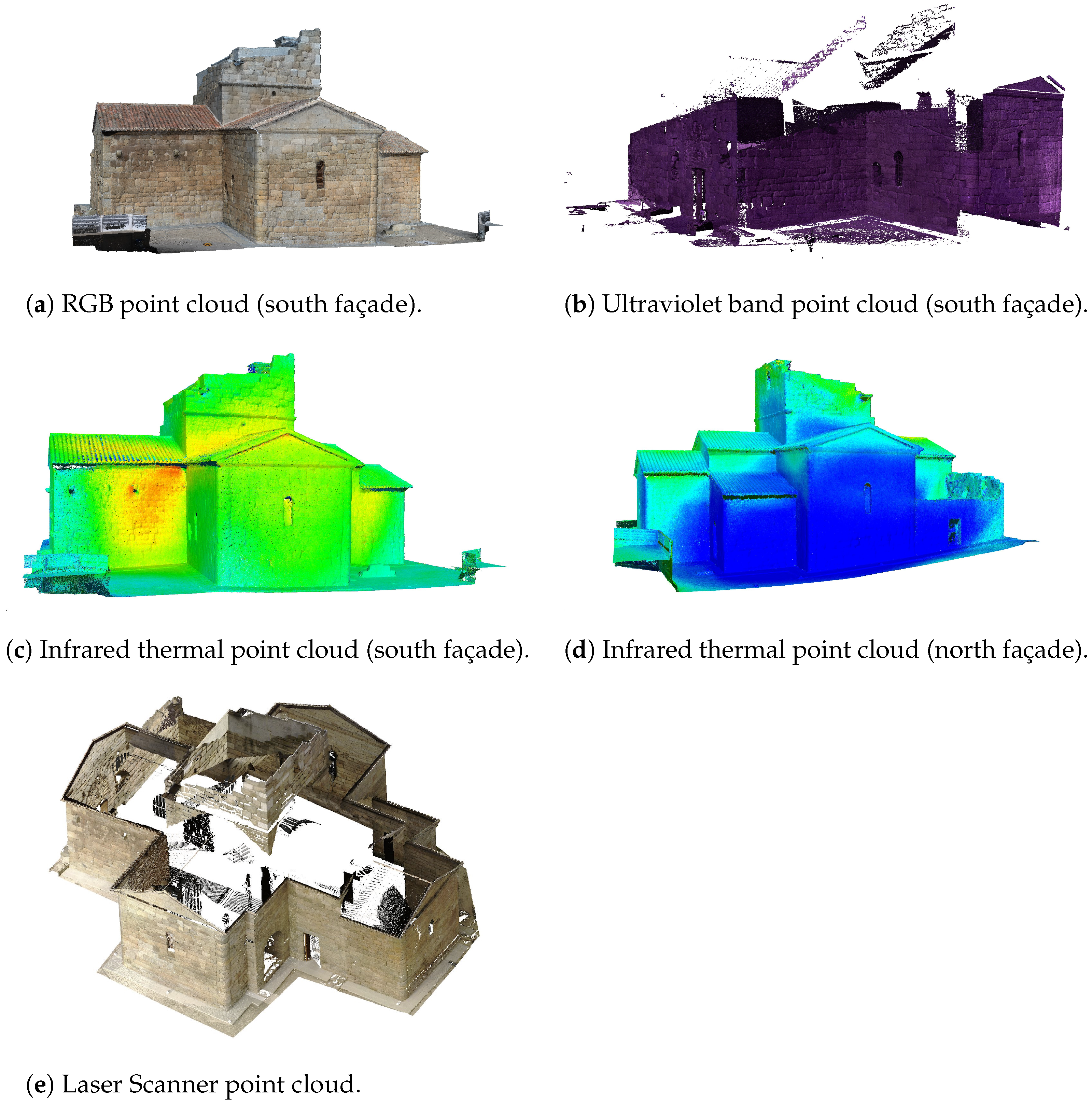
Figure 9 illustrates a subset of the point clouds views resulting from the use of the aforementioned sensors. First,
Figure 9a presents a visualization of the point cloud obtained via RGB sensors using both conventional terrestrial and aerial (UAV) cameras. This representation unveils architectural details as well as visible features perceptible to the naked eye, furnishing a meticulous view of the surface of the structure. This point cloud has been selected as the starting point for the development of the voxelized data structure of the building in question, which will be subjected to analysis in subsequent stages.
Figure 9b shows the point cloud corresponding to the UV spectral band. This view allowed us to identify elements that are typically imperceptible within the visible range. In this
Figure 9b we also can see that not the entire building has point cloud information in this band.
Finally, in
Figure 9c,d, we depict the point cloud generated by our infrared thermal sensor. This visual representations highlight the heat distribution on the building surface, endowing us with an exceptional perspective concerning potential issues related to heat retention and the variability of construction materials.
Beyond the previously outlined difficulties concerning data structure, heterogeneity, and inconsistent density, point clouds generated by multiple sensors emanate from disparate data origins and convey unique informational facets. Consequently, it becomes essential to formulate strategies for the fusion of both geometric and spectral elements with the aim of optimizing data processing and extracting valuable conclusions from the varied information contained within.
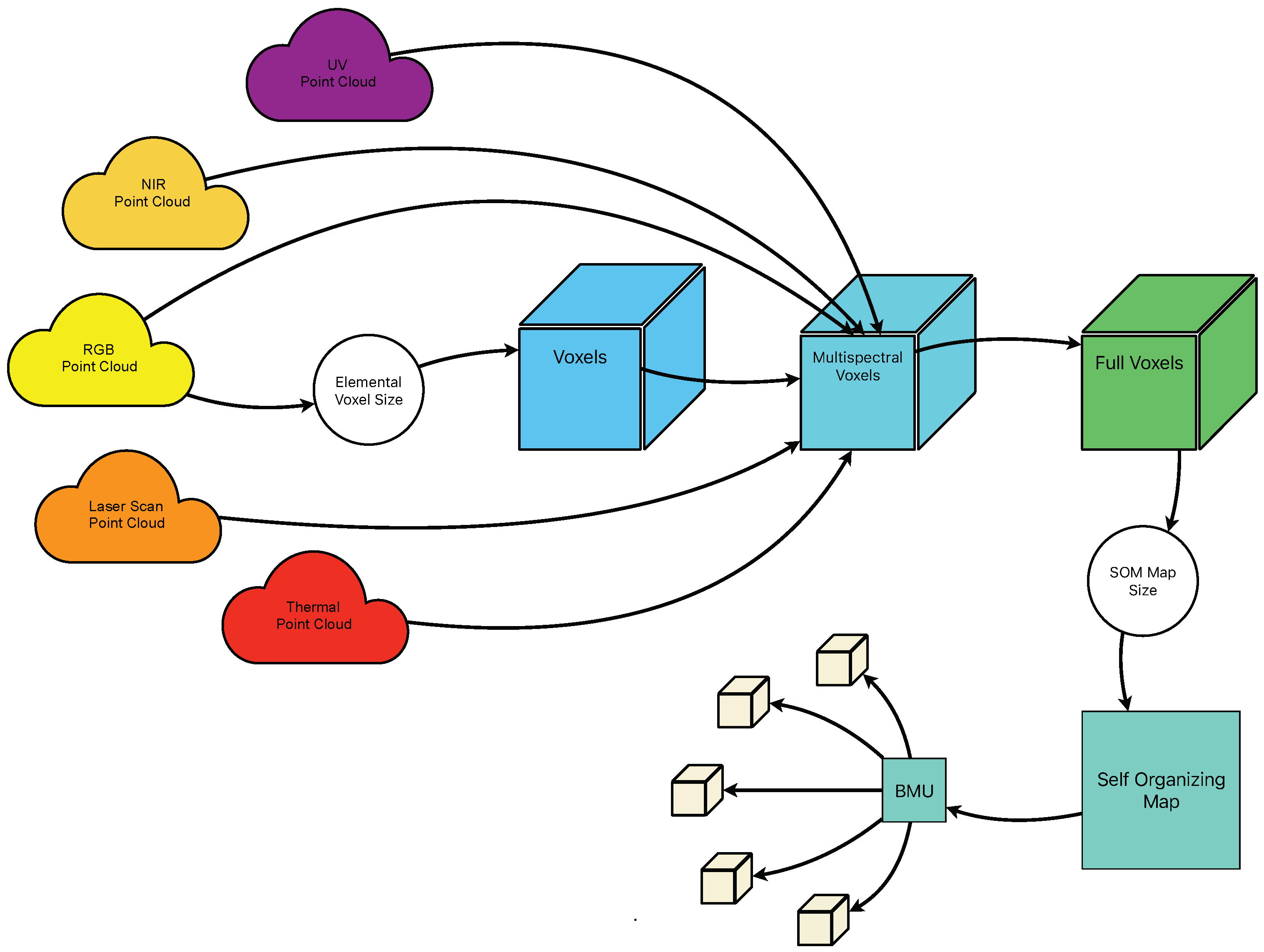
2.4. Voxelization
To facilitate an optimal analysis, it is necessary to fuse the numerous point clouds that have been generated. To accomplish this, we have employed voxels as the data structure, specifically the multispectral voxel variant developed in our previous research [
29].
Voxels, abbreviated from “volumetric elements”, serve as the fundamental abstract units in three-dimensional space, each having predetermined volume, positional coordinates, and attributes [
63]. They offer significant utility in providing topologically explicit representations of point clouds, thereby augmenting the informational content.
In this study, we examined how the selected elemental voxel size affects the point distribution within the point clouds. Voxel structures with various elemental sizes (50, 25, 10, 5, and 3 cm) were created. To manage the point clouds and their voxelization, we used the Open3d open-source library [
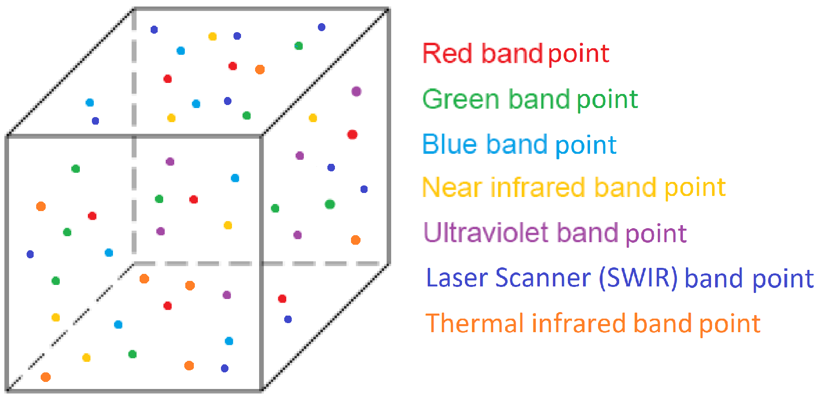
64]. We used the RGB point cloud as the initial dataset to create voxel structures, given its comprehensive coverage of the entire building. After establishing voxel structures based on these sizes, we located the points from each respective cloud enclosed within individual voxels. In instances where one specific voxel enclosed multiple points from a particular spectral band, the voxel’s spectral property was set to the mean value of those enclosed points. Additional statistical metrics, such as the maximum, minimum, and variance values, were also calculated. Given that the voxel adopts the spectral attributes of enveloped points, it effectively becomes a multispectral voxel [
29]. The concept of a multispectral voxel used in this work is illustrated in
Figure 10.
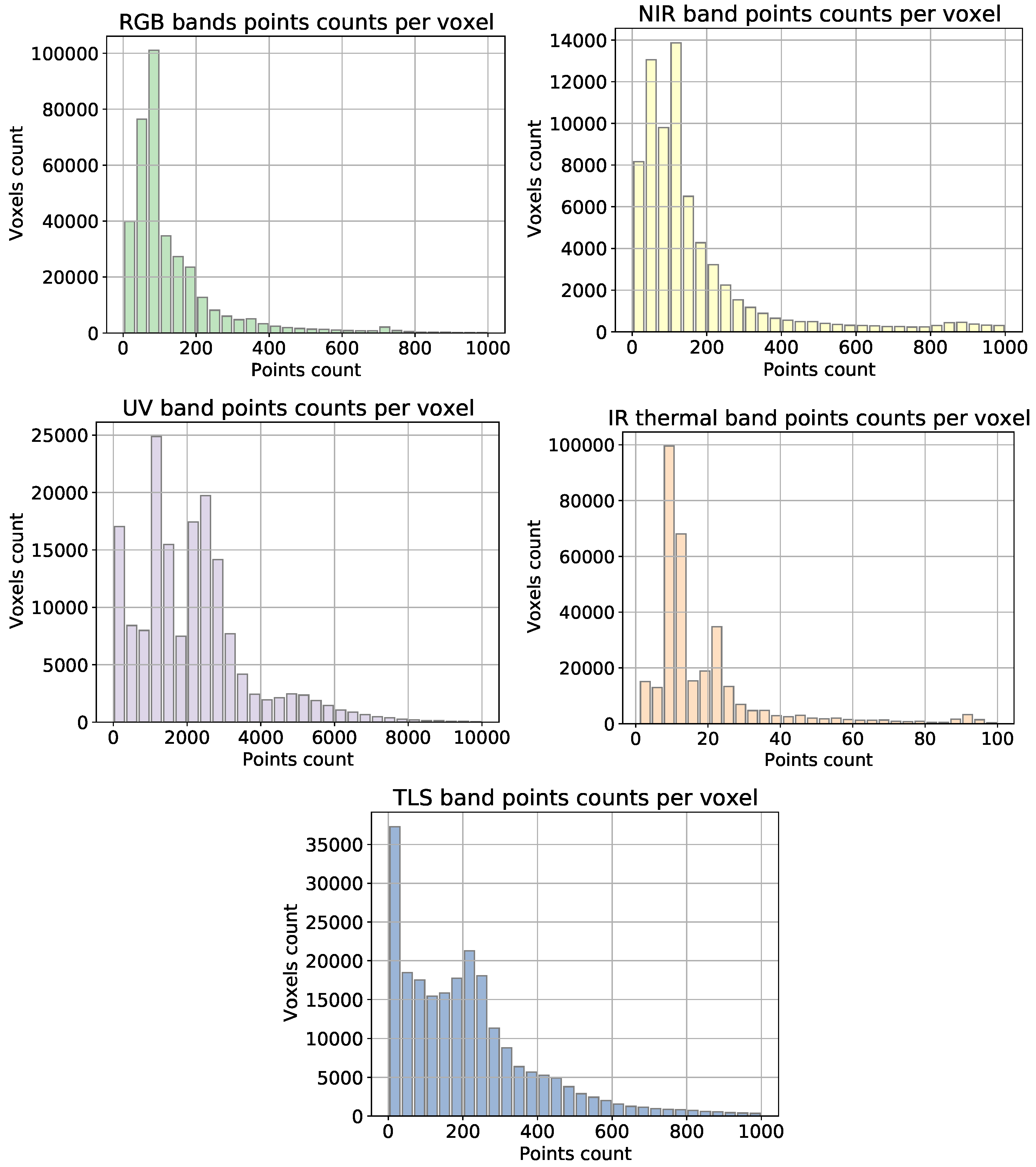
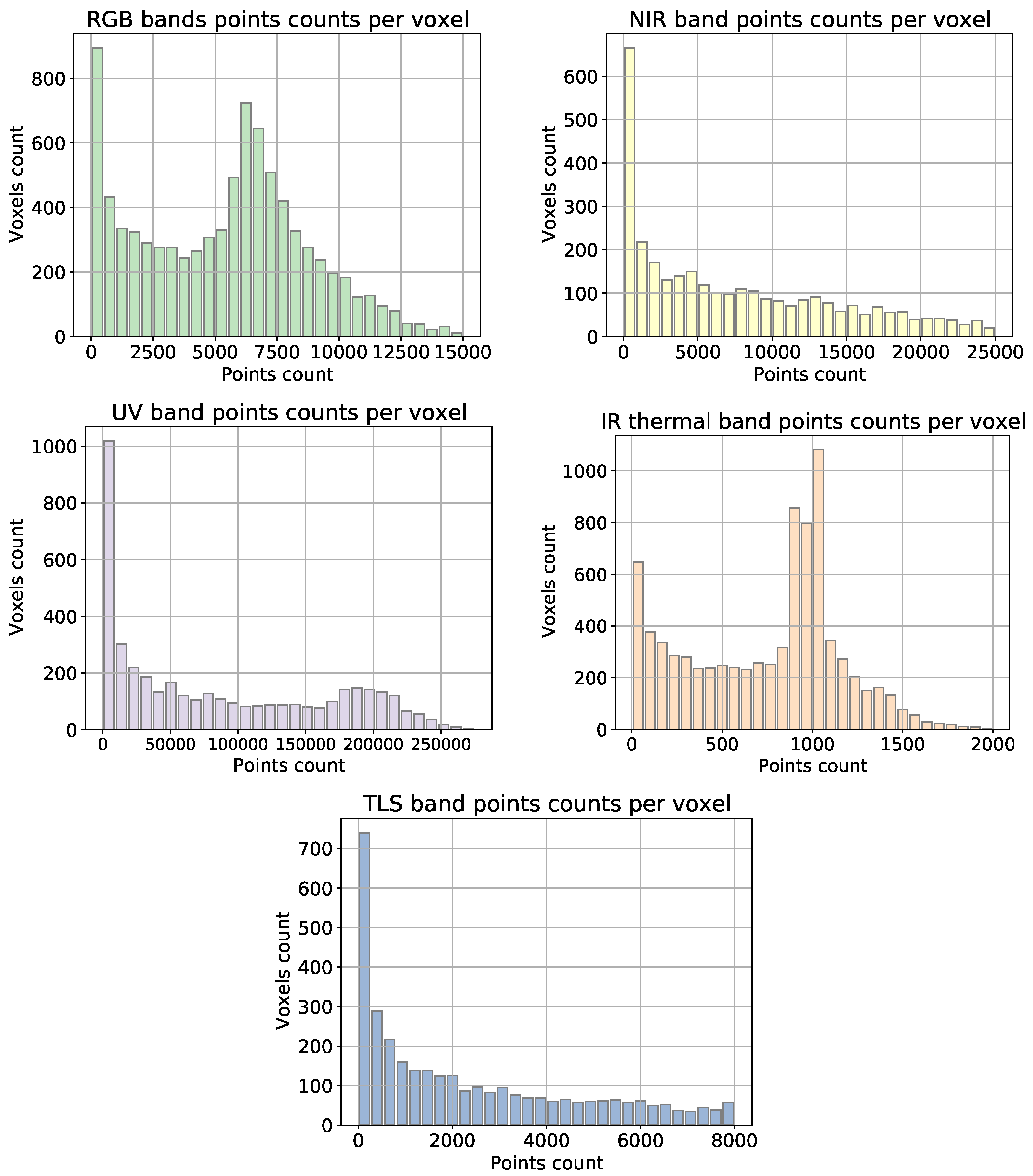
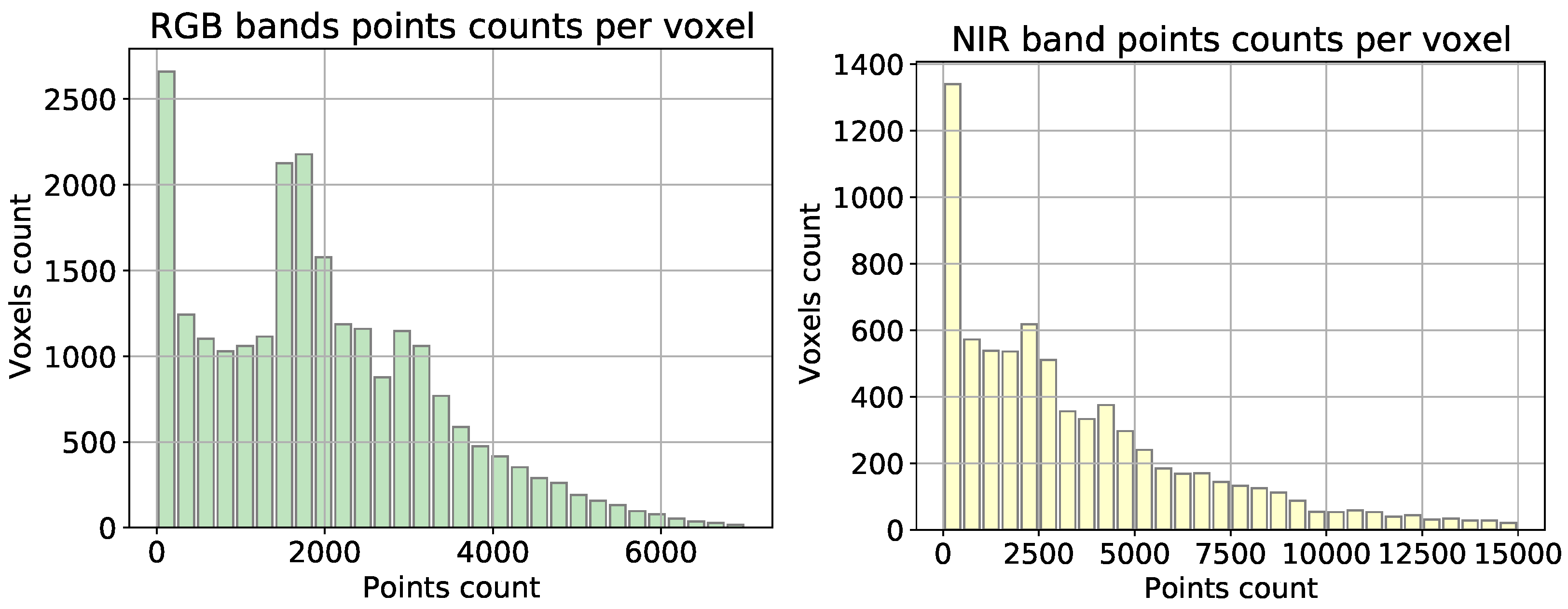
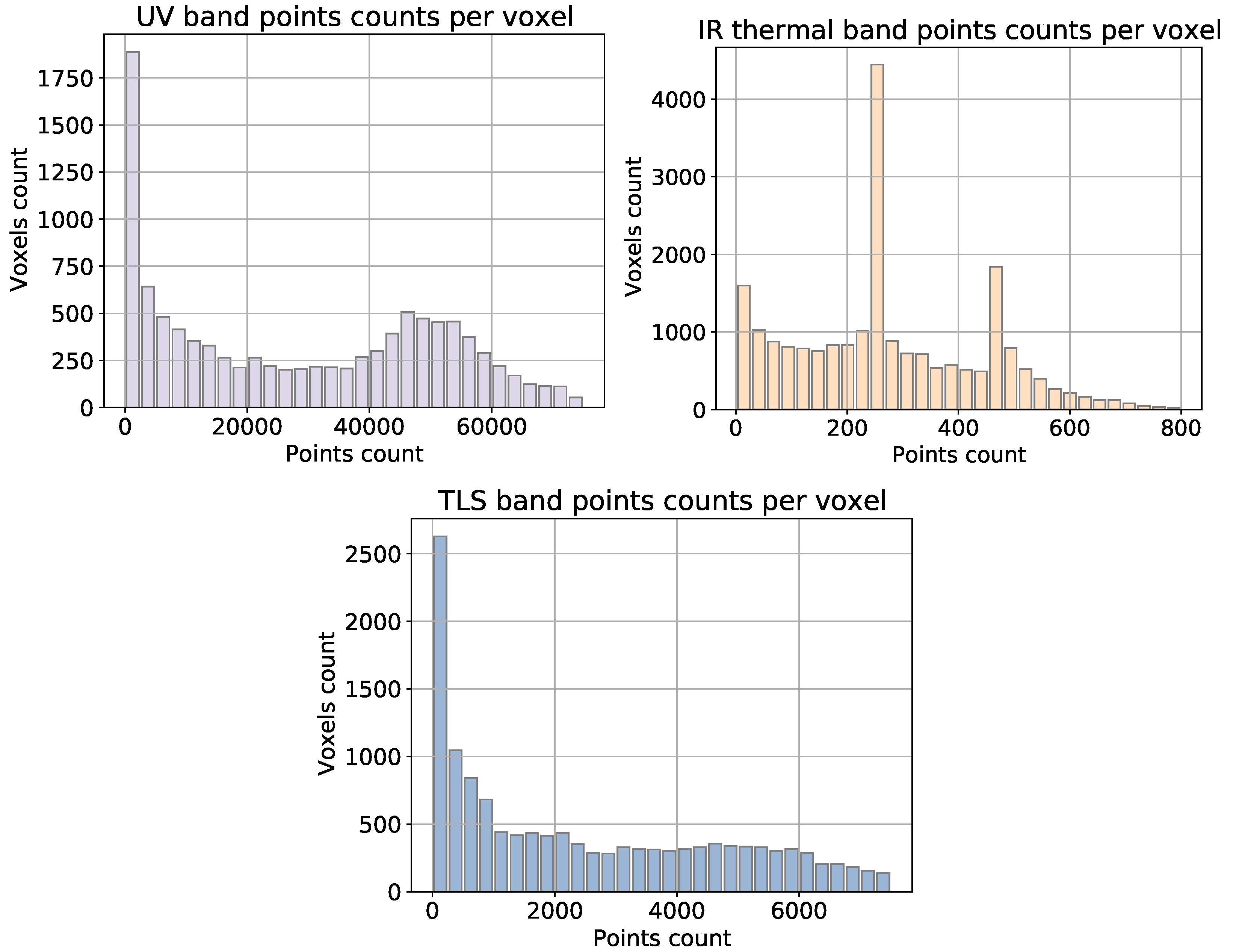
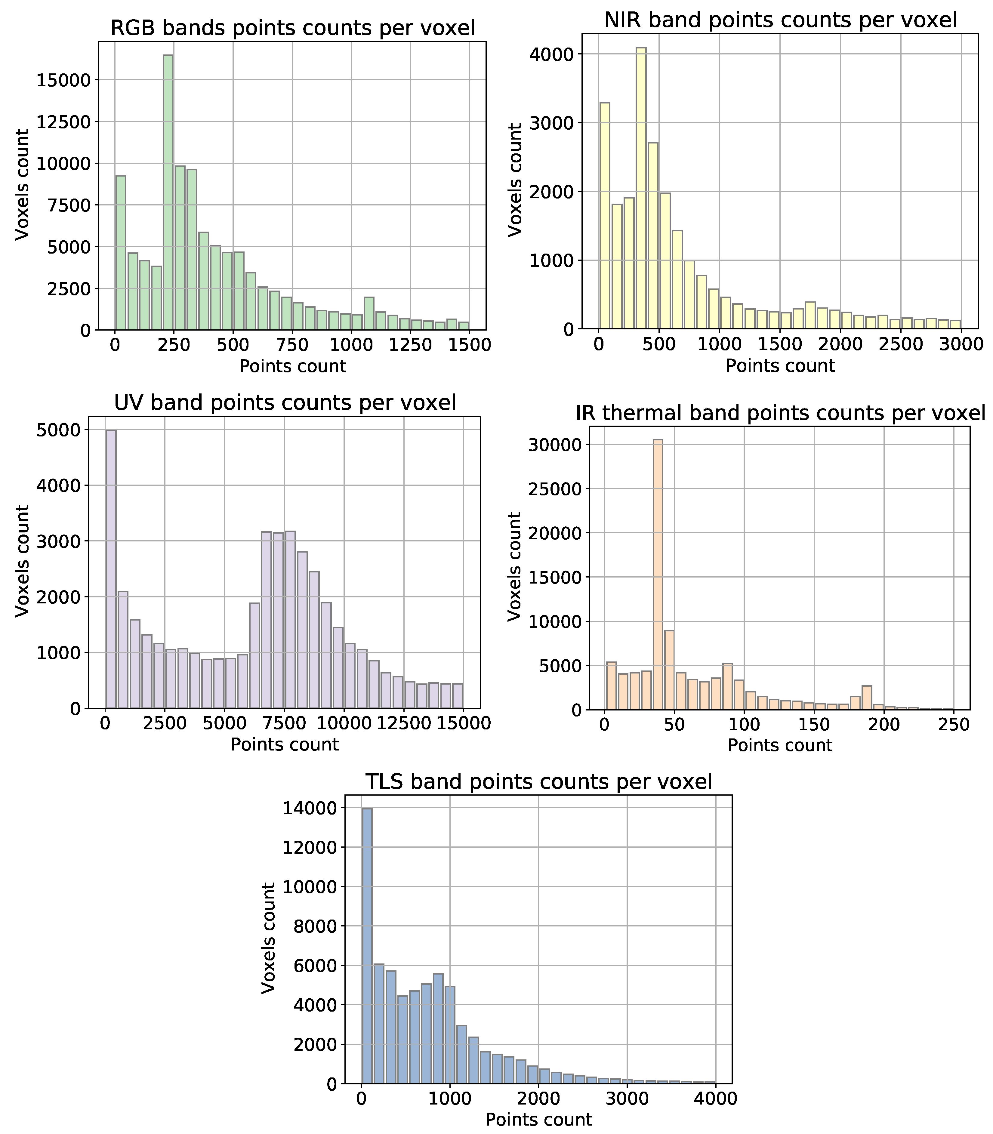
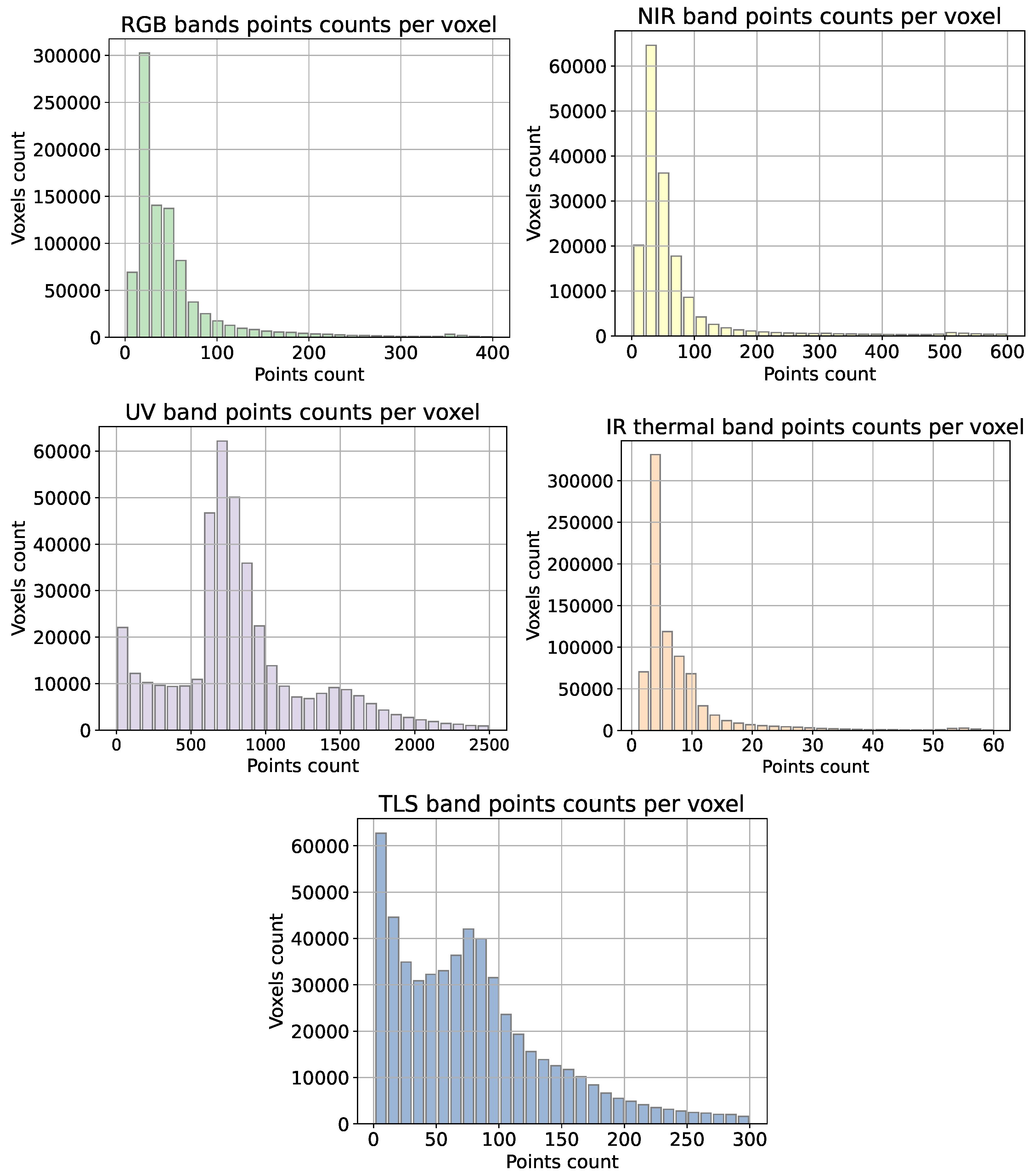
Figure 11 illustrates how point clouds are distributed along the 5 cm elemental voxel structure. For other chosen voxel elemental sizes, please refer to
Appendix A, where we provide the respective distributions. The histograms in
Figure 11 show the number of points per voxel in each spectral band.
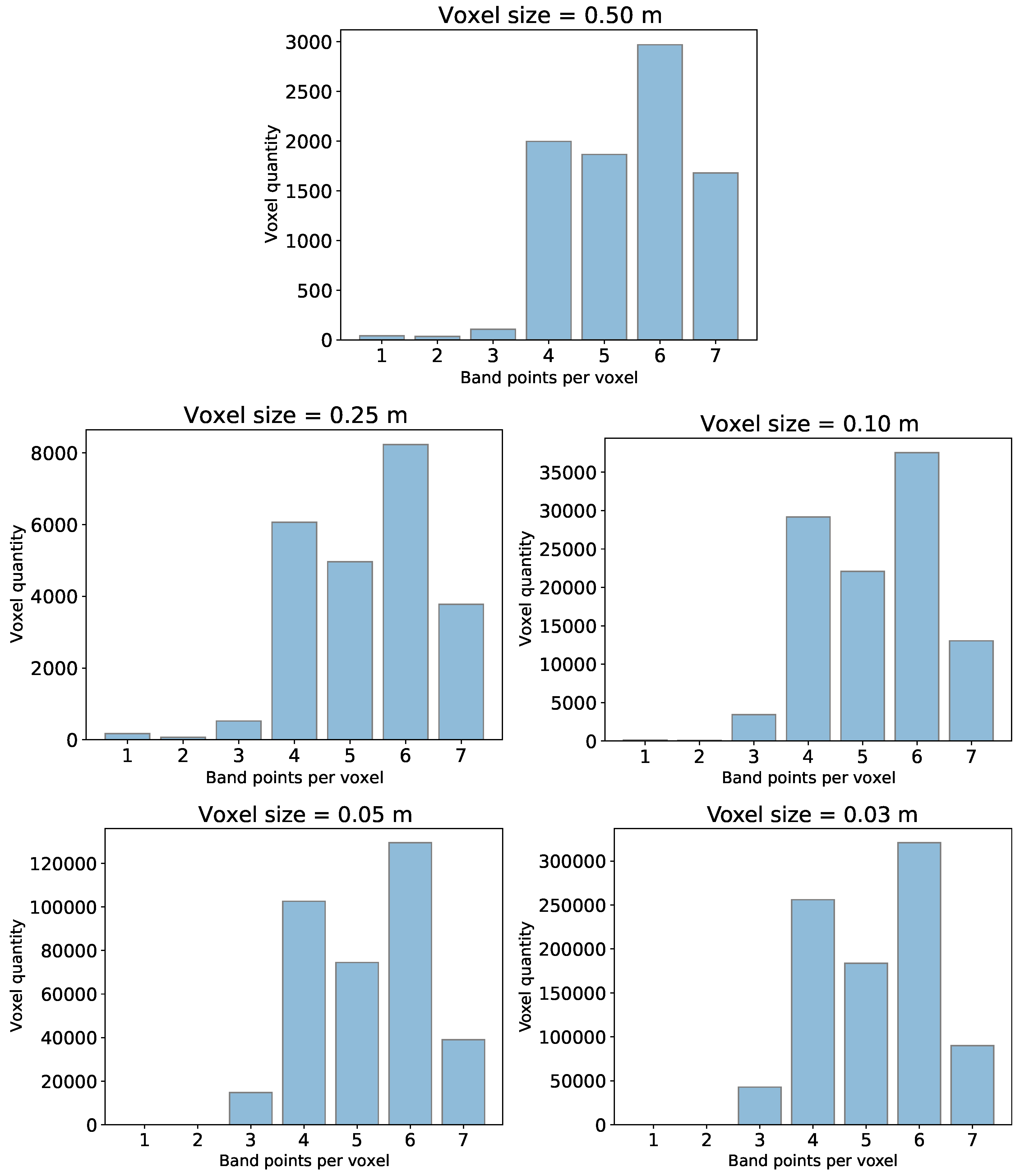
We have also carried out an analysis of the influence of the size of the elementary voxel with respect to the number of points contained. We can observe their distribution in the form of histograms in
Figure 12. We note that the distribution of the spectral bands contained in the multispectral voxels does not depend specifically on the elemental voxel size, as the distributions outlines are similar.
Once the structure of multispectral voxels is established, it is crucial to process this data to gain insights and draw conclusions about the target building under study. In this research work, we have opted for the implementation of Self-Organizing Maps (SOMs) algorithms, due to their multiple advantages in handling voxel data. SOMs provide an efficient summarization of data, facilitating understanding, especially when dealing with large datasets, thus excelling in dimensionality reduction tasks. They do not require a separate training phase and are adept at exploiting spatial attributes while maintaining local neighbourhood relationships. With a design that is more intuitive than other neural network types, SOMs ease the interpretation of generated outcomes, making them particularly suitable for tackling categorization problems.
2.5. Self-Organizing Maps
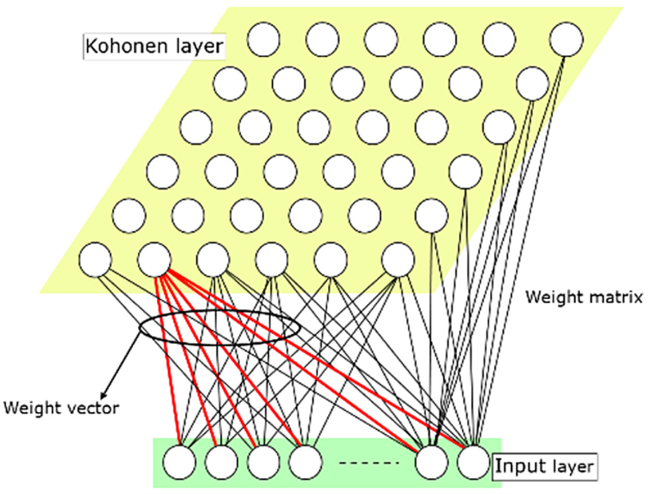
The Self-Organizing Map (SOM) executes a transformation from an input space of higher dimensionality to a map space of lower dimensionality, using a two-layered, fully interconnected neural architecture. The input layer comprises a linear array of neurons and the elementary units of an Artificial Neural Network (ANN), and the number of these neurons corresponds to the dimensionality of the input data vector (
n). The output layer, also known as the Kohonen layer, is composed of neurons, each possessing a weight vector that matches the dimensionality of the input data (
n). These neurons are organized within a rectangular grid of arbitrary dimensions (
k). The weight vectors are collectively represented in a weight matrix configured as an
array [
65].
Figure 13 illustrates the typical Kohonen map architecture.
Among the various features provided by the use of SOMs are the following:
Group together similar items and separate dissimilar items.
Classify new data items using the known classes and groups.
Find unusual co-ocurring associations of attribute values among items.
Predict a numeric attribute value.
Identify linkages between data items based on features shared in common.
Organize information based on relationships among key data descriptors.
It has been proven that SOMs need complete data records [
66]. SOMs are highly sensitive to Nan values and empty fields in the input layer. For this purpose, only full voxels, that is, those with at least one point contained in each of the point clouds to be fused, were classified in our training.
SOM Quality Indices
The various parameters that define a SOM can lead to different neural spaces. SOM quality measures are required to optimize training, such that meaningful conclusions can be drawn from them. Among these, the most significant quality indices are:
Quantization error is the average error made by projecting data on the SOM, as measured by euclidean distance, i.e., the mean euclidean distance between a data sample and its best-matching unit [
67]. Best value of quantization error is zero.
Topographic product (TP) [
68] measures the preservation of neighborhood relations between input space and the map. It depends only on the prototype vectors and map topology, and can indicate whether the dimension of the map is appropriate for fitting the dataset, or if it introduces neighborhood violations, induced by foldings of the map [
67]. Topographic product will be <0 if map size is small and >0 if map size is big. Best value will be the one with the lower absolute value.
In this work, SOM quality indices have been calculated using an open-source library, SOMperf [
67].
To determine the optimal neuron map size (k), Topographic Product (TP) [
68] has been used. An approximation corresponding to a rule of thumb, according to Equation (
1):
being
N the number of full voxels in the voxelized structure.
In
Figure 14 we summarize in a flowchart the handling of the processed data during our multisensor data fusion strategy.
3. Results
SOM trainings was performed for each voxel size. For this purpose, the optimal map size was determined such that the topographic product was minimum (in absolute value).
Table 7 lists the different parameters according to the voxel size, as well as the obtained topographic product and quantization error.
One of the first steps prior to training is the normalization of the data. Normalization helps the features to have a similar scale, facilitating the training process and faster convergence. In addition, normalization helps to avoid problems associated with large gradients during training, which negatively affect model convergence. In our work, we conducted a Min-max rescale normalization.
To illustrate, we will concentrate on the presentation of the SOM outcomes for a voxel size of 5 cm (0.05 m). The varied results of the maps according to the voxel size are organized in
Appendix A.
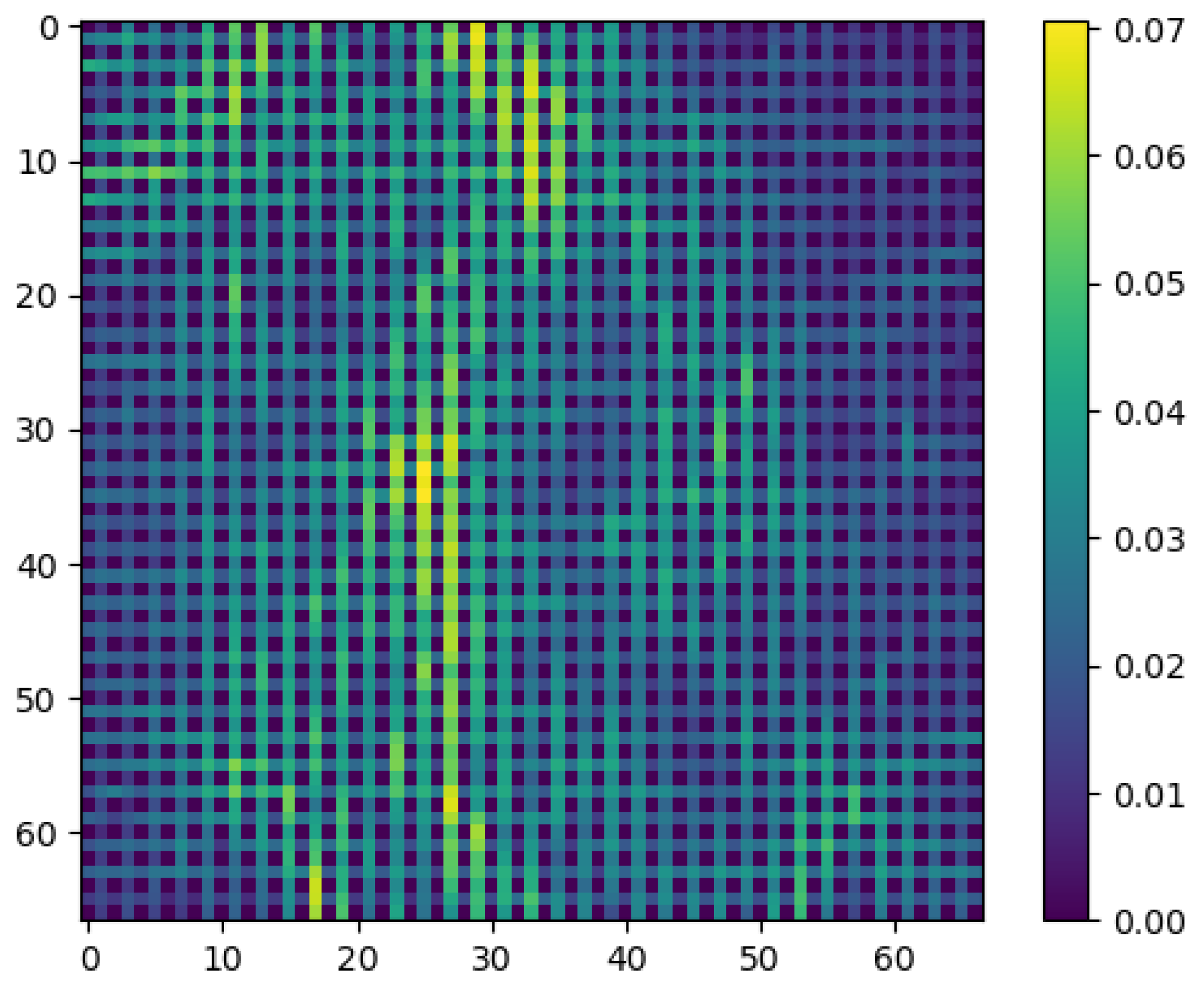
As shown in
Figure 13, the results of the training and classification of a self-organized map are provided by a matrix of neurons, which are assigned a series of weights given by the input layer. One way to show the relationships between neurons is to express the distances between them (
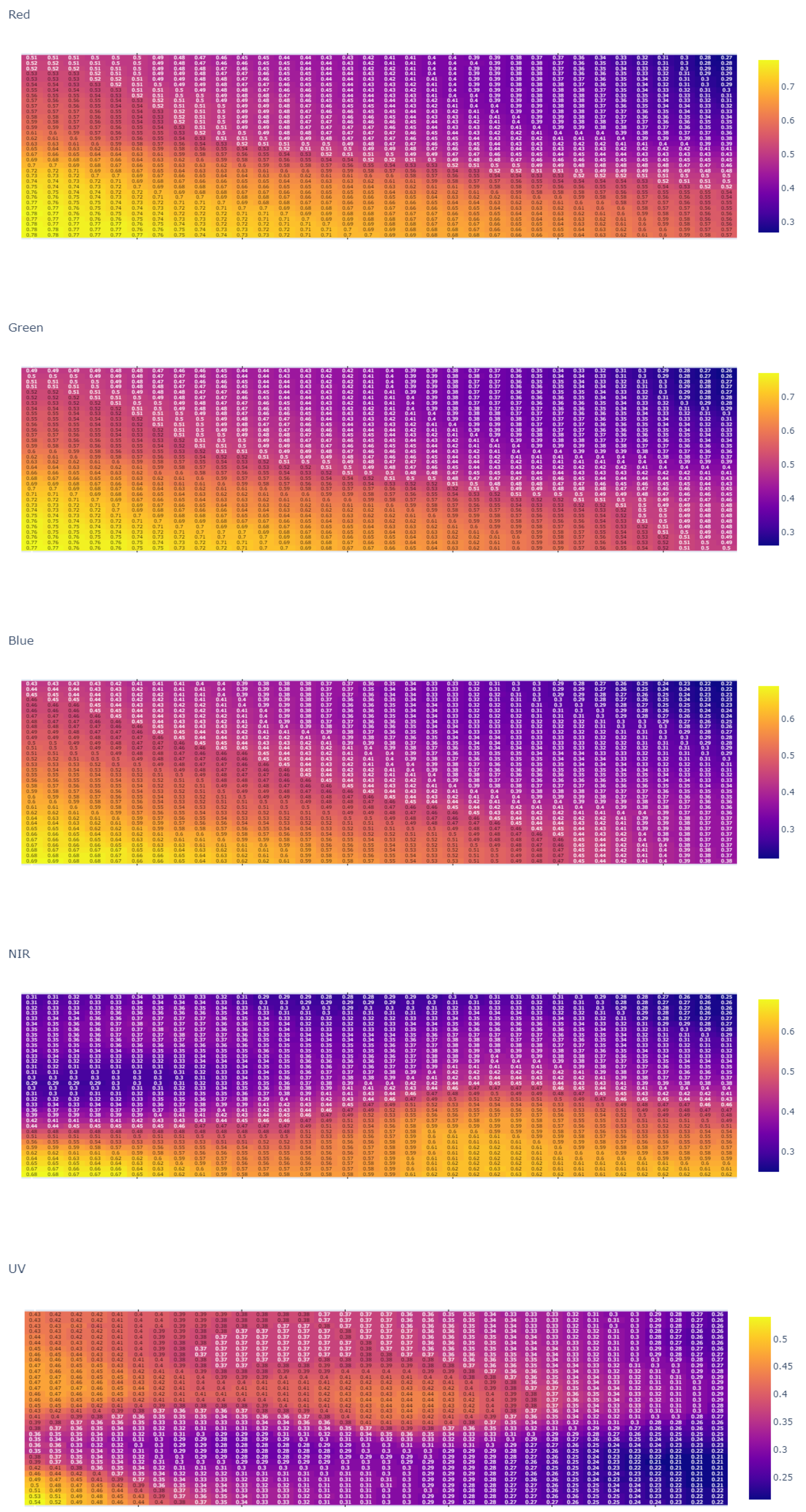
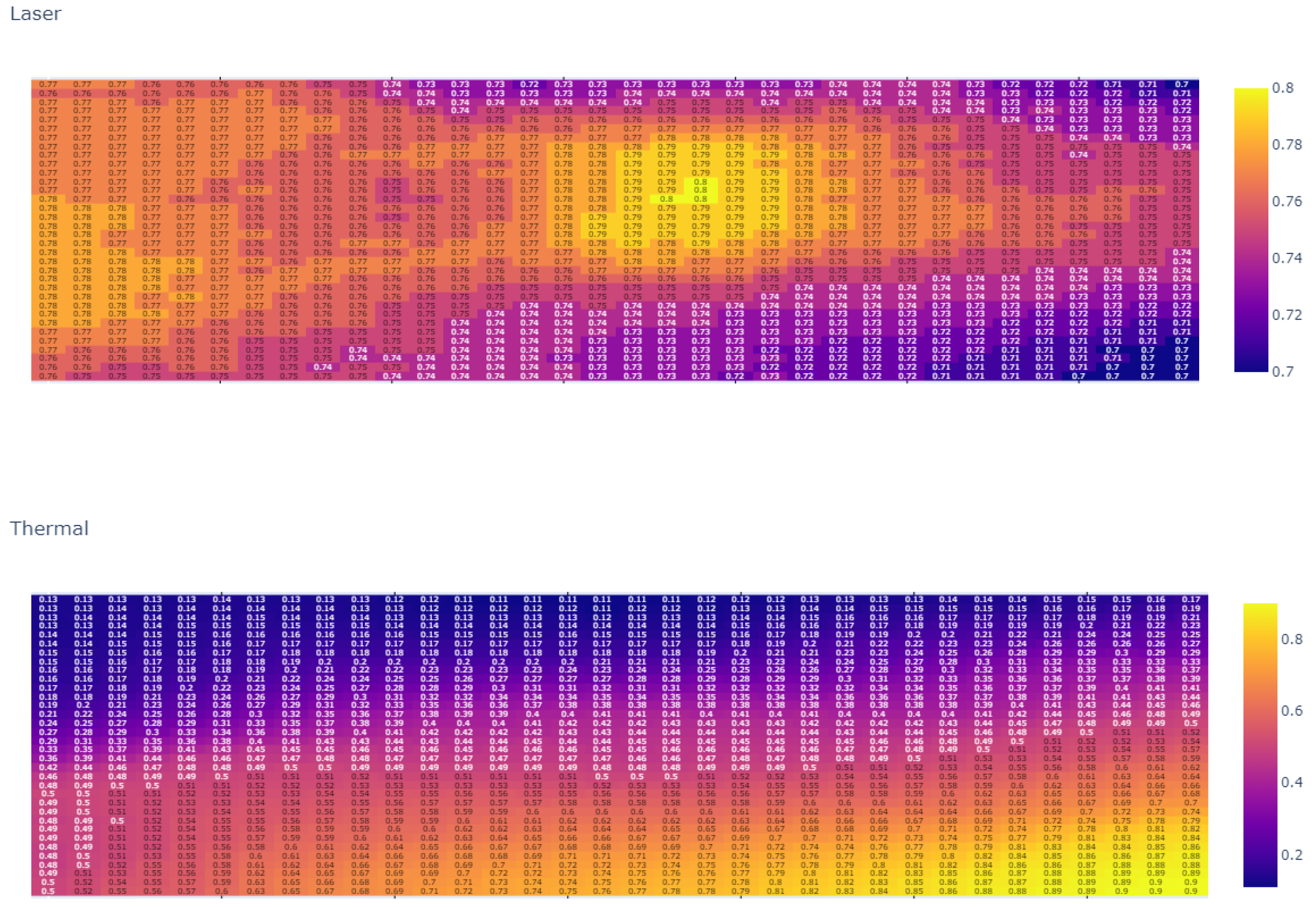
Figure 15). The lighter parts in that matrix represent the parts of the map where the nodes are far away from each other, and the dark parts represent less distance between nodes.
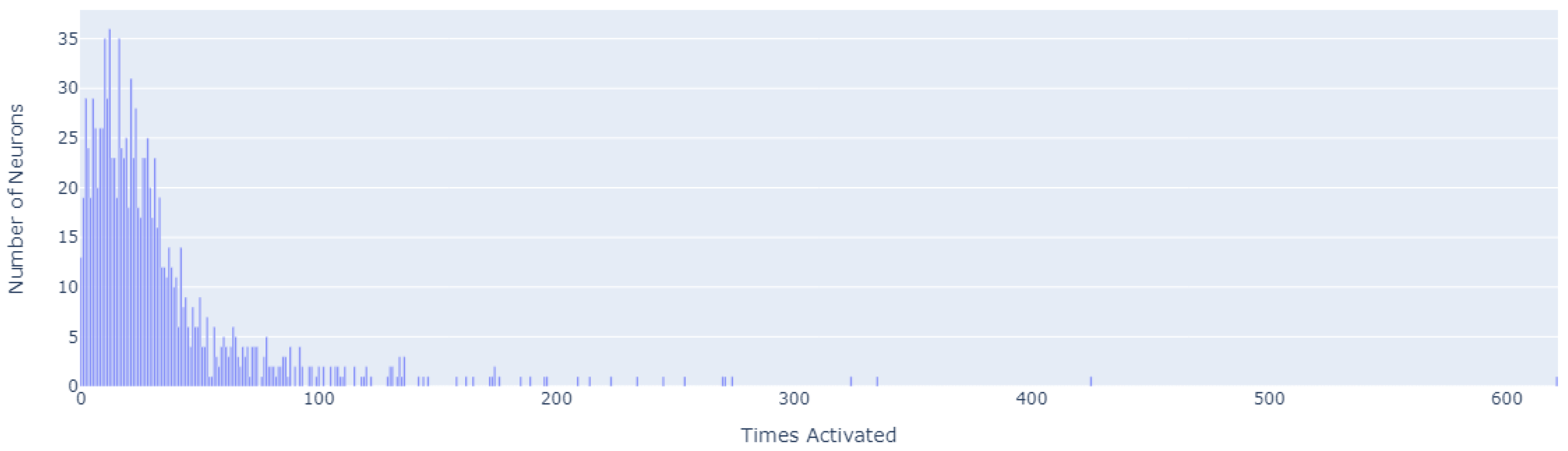
Each activated neuron represents a set of voxels. There are also neurons that have not been activated by any of the vectors given by the multispectral voxels within the input layer.
Figure 16 shows how many patterns (
x-axis) have been recognized by how many neurons (
y-axis).
The distribution of activations can be seen in the activation map depicted in
Figure 17.
In the same way, we show how the activations of the neurons are distributed within each codebook vector (
Figure 18).
4. Discussion
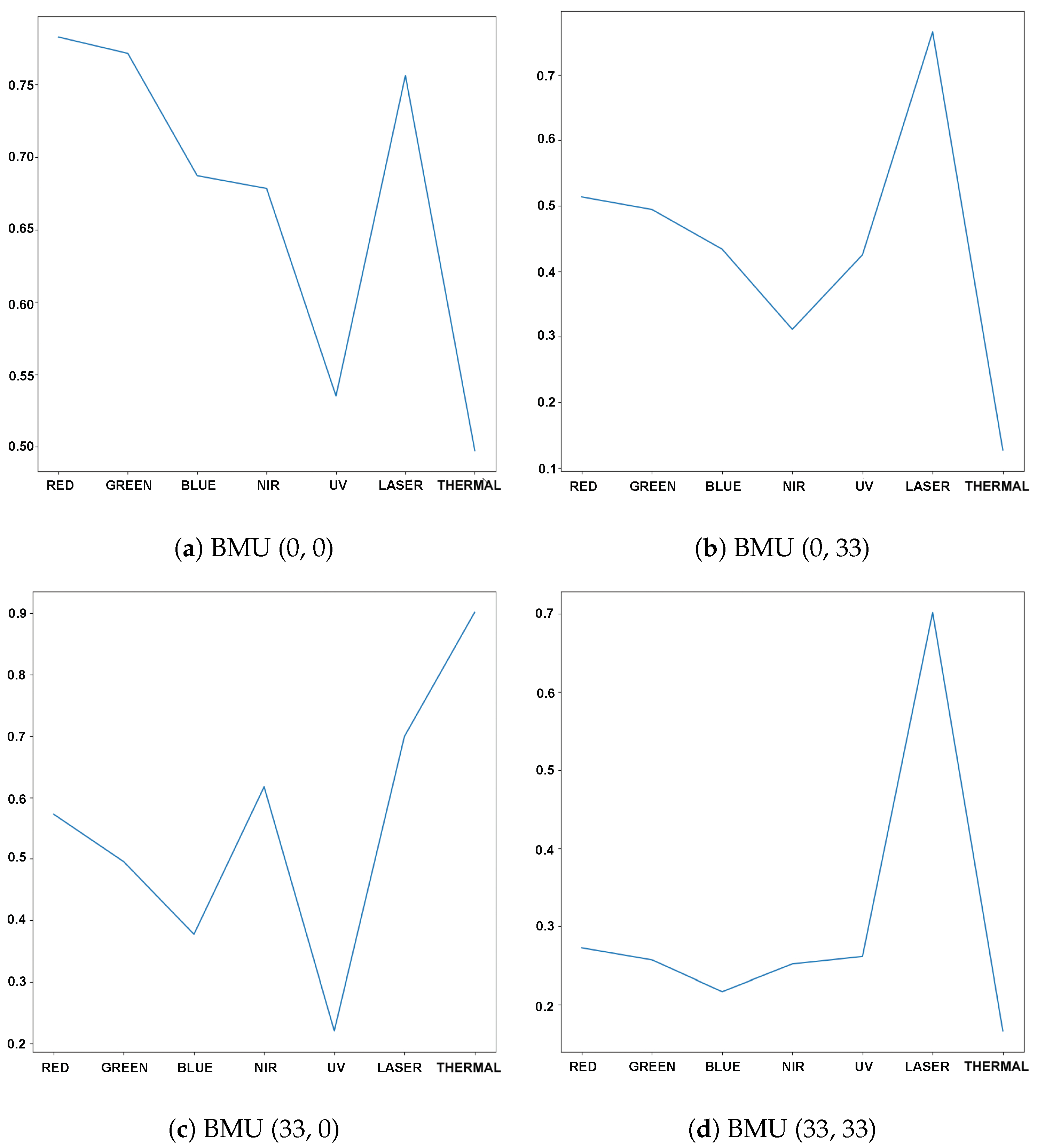
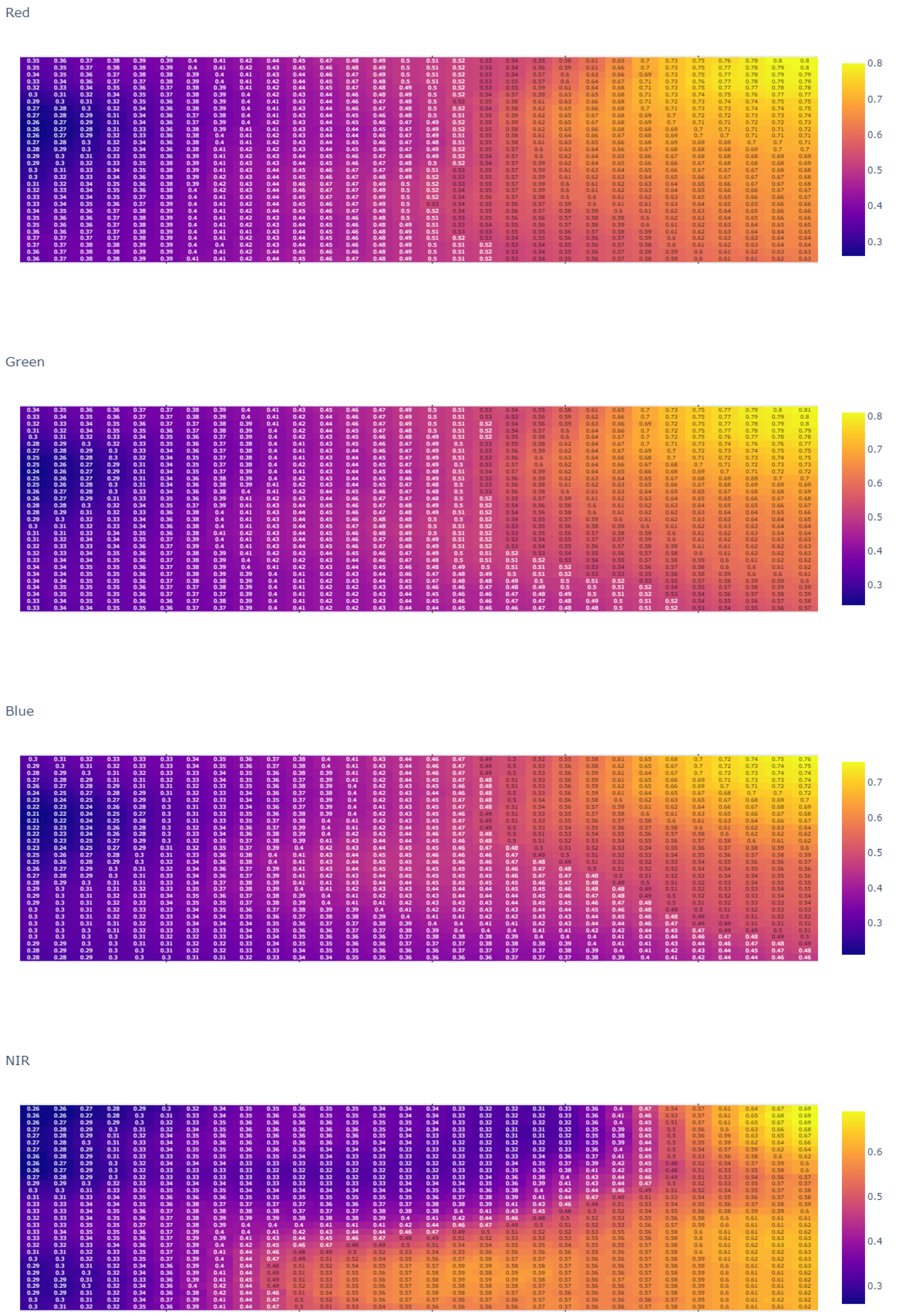
The use of Self-Organizing Maps (SOM) for the training and classification of multispectral voxel structures results in the generation of a neural map. In this map, each neuron points towards a group of voxels that exhibit similar characteristics, as indicated by a vector of weights assigned to each property (spectral band) of the input layer. Every voxel in the input layer has a Best Machine Unit (BMU). The BMU is the neuron whose weight vector is closest in the space to the pattern.
In the SOM heat map voxel 5 cm (
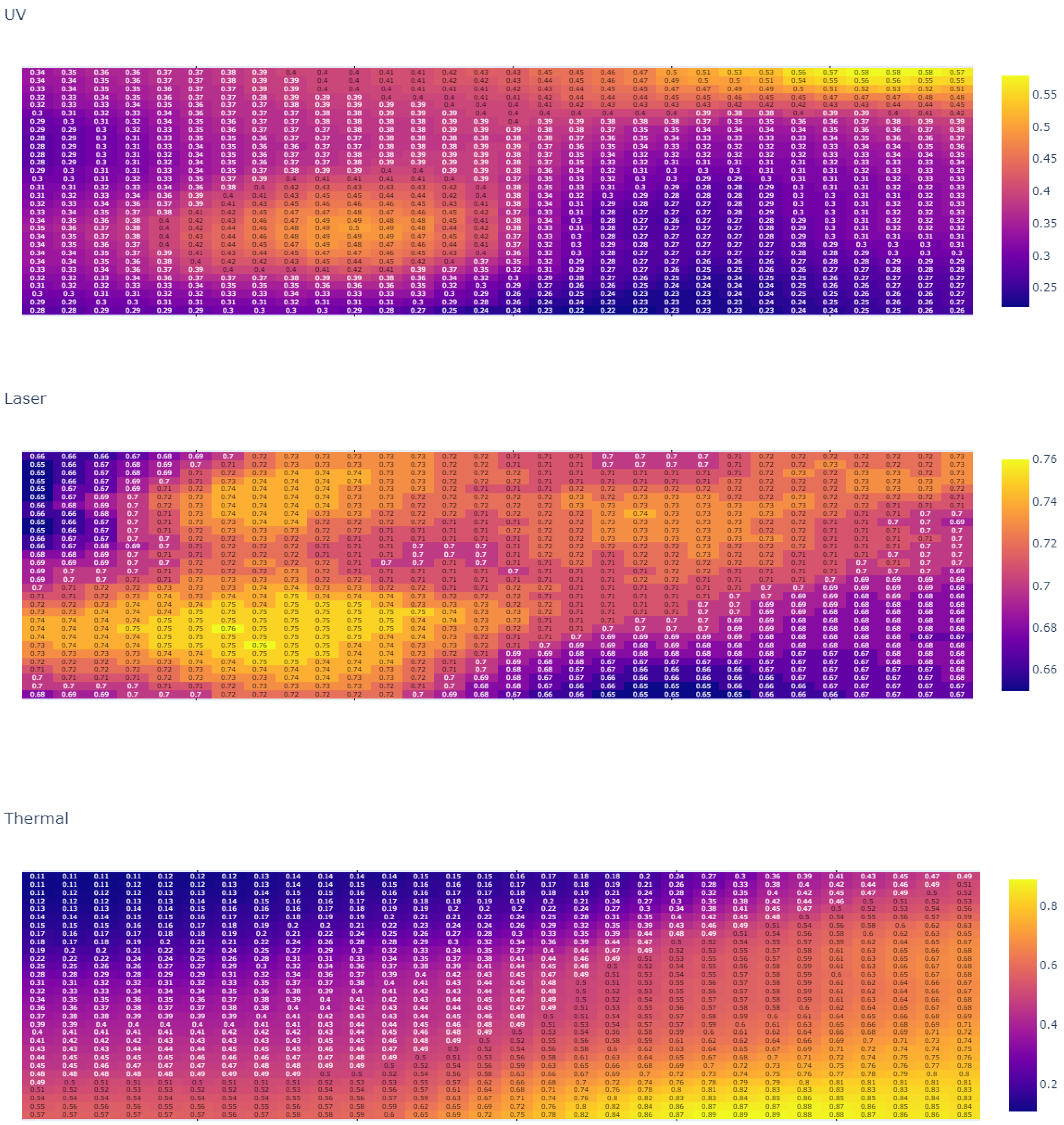
Figure 17), we can identify which neurons are those that determine clearer patterns because they have been activated a greater number of times. We highlight the neurons in the corners of the heat map.
Neuron (0, 0), activated by 274 voxels. The red band is the predominant band, together with the laser. The UV and thermal bands have less weight for these voxels (
Figure 19a). These activated voxels are mostly located on the south building façade.
Neuron (0, 33), activated by 425 voxels. Its most important band is the laser band. The rest of the bands (RGB and UV) show a medium weight, whereas the thermal information has little influence (
Figure 19b). Its voxels are located on the western planes not illuminated by the Sun during data acquisition.
Neuron (33, 0), activated by 621 voxels. Its characteristic band is the thermal band, with a minimum in the UV band. The red and green bands, along with the NIR have medium weights. The laser band also has considerable weight (
Figure 19c). The voxels targeted by this neuron are located on the northern façade.
Neuron (33, 33), activated by 136 voxels. Larger weight of the laser band. The rest of the bands (RGB, NIR, UV, and thermal) have lower weights (
Figure 19d).
However, each neuron does not act in isolation, but interconnects with nearby neurons (
Figure 15). Nearby neurons interrelate similar multispectral voxels. As shown in
Figure 18, neurons can be zoned using cross-band interrelated weights. In our analysis, we have observed a striking similarity in the distribution of weights of the neurons in the heatmap, corresponding to the red, green, and blue bands, located in the lower left corner. This finding can be attributed to the fact that the built-up area of the building, as depicted in
Figure 5, primarily exhibits a red-grayish tone, derived from the granite construction.
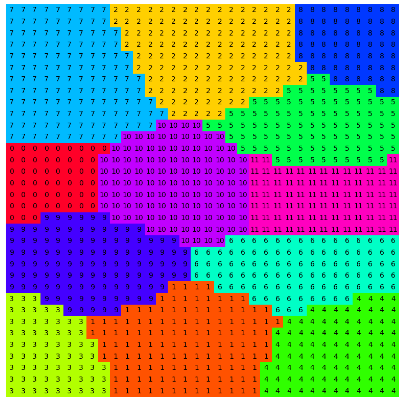
This distribution of weights presents an opportunity for further analysis. Employing a clustering algorithm, as the K-means method, we have successfully segmented the BMUs. Using, for example, a 12-zone clustering, we are able to identify similar BMUs in a manner that considerably streamlines analysis and enhances decision-making (
Figure 20).
The primary focus of our methodology is to identify and study building pathologies through the fusion of geomatic sensor data. We identified an area with dampness in the building that was examined. This area is located in the lower part of one of the northern façades (
Figure 21). Dampness in buildings can lead to various issues such as the formation of salt efflorescence. These are white deposits on the surfaces resulting from the migration of soluble salts in water through the pores of the construction materials. This phenomenon often occurs when water carries salts from the ground to walls. In addition to efflorescence, moisture can trigger mold growth, material deterioration, and structural problems [
69].
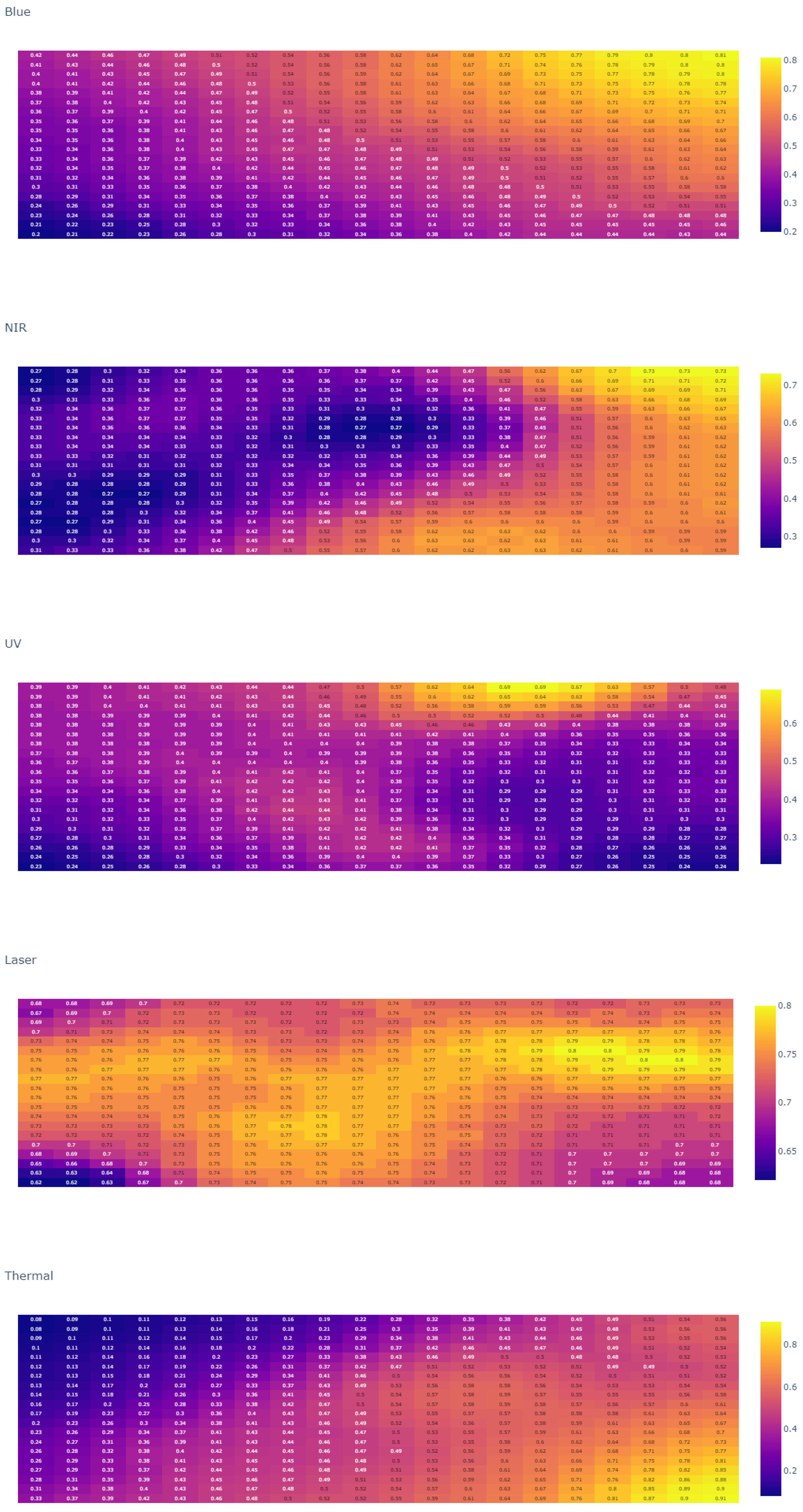
In order to evaluate our hypothesis regarding the potential application of multispectral voxels in multisensor data fusion for the purpose of studying building pathologies through the use of self-organizing maps (SOMs), we specifically focused on the voxels that represented areas of the building with pathology present. We then identified the best matching units (BMUs) for these voxels and discovered that they were located in close proximity to the neuron (33, 20). To confirm the validity of their weight vector, we obtained the corresponding characteristic graph, shown in
Figure 22. The graph indicates a strong correlation between the visible spectrum bands and the laser scanner band.
Earlier research in remote sensing building pathologies studies discovered that the infrared spectral range, particularly the 778, 905, and 1550 nm wavelength bands, is ideal for detecting dampness. The study [
1] found that the best results were obtained using short-wave infrared data (1550 nm). Visible wave bands can detect efflorescence, as surfaces with this phenomenon have higher reflectance in these spectral ranges. For chlorides or sulphates being the cause, the short-wave infrared range is more appropriate. In accordance with the research conducted by [
1], our methodology demonstrates a higher level of effectiveness as it does not rely on the derivation of information from point clouds to images to localize and study pathologies. Instead, we work directly with the original 3D point clouds, integrating geospatial 3D geometry with multispectral data information.

 ,
, 


