
Preserving Colour Fidelity in Photogrammetry—An Empirically Grounded Study and Workflow for Cultural Heritage Preservation
 , , and
Abstract
:1. Introduction
2. Related Work
2.1. Colour Perception in Cameras
2.2. Colour in Material Cultural Heritage
2.3. Cultural Heritage 3D Models
3. Materials and Methods
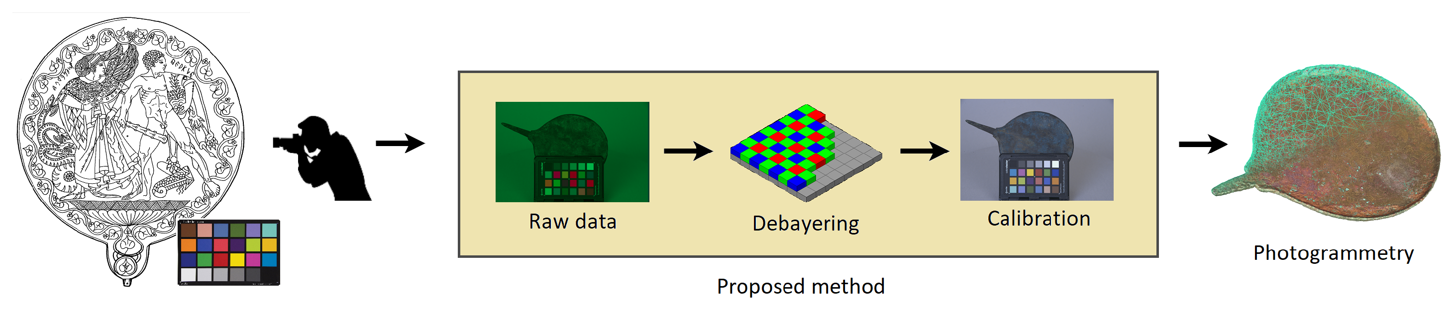
- 1.
- Debayering: recover RGB data from the raw file.
- 2.
- Calibration: surpass perceived chromatic differences.
- 3.
- Photogrammetry: build the Cultural Heritage model starting from a calibrated batch of images.
3.1. Debayering
- 1.
- Direct debayering: Direct debayering of the raw image data of the NEF format based on standard procedure following the Python RawPy library [22]. Its concrete algorithm is “Adaptive homogeneity-directed demosaicing algorithm” (“AHD”). It features the advantage of estimating the colour by minimizing artifacts and errors; however, its conception based in filter banks makes the process non-linear, and additionally loses a small stripe of pixels due to convolution operations [23].
- 2.
- Bilinear interpolation: respecting the original pixel size of the raw image, the non-valid pixels are substituted by a bilinear interpolation of the Bayer tiles pixels. It has the advantages of linearity—and therefore reversability—and the fact that the full size of the image is saved. The disadvantage may be a bigger risk of the production of colour artifacts due to its simple conception.
- 3.
- Discard: all non-valid pixels are discarded, and the resulting image is one quarter of the size of the original raw file. Its obvious advantage is that no new information is fabricated, therefore all saved pictures bear true information. The disadvantage is effectively, the loss of information, while it may ease calculations due to its reduced size.
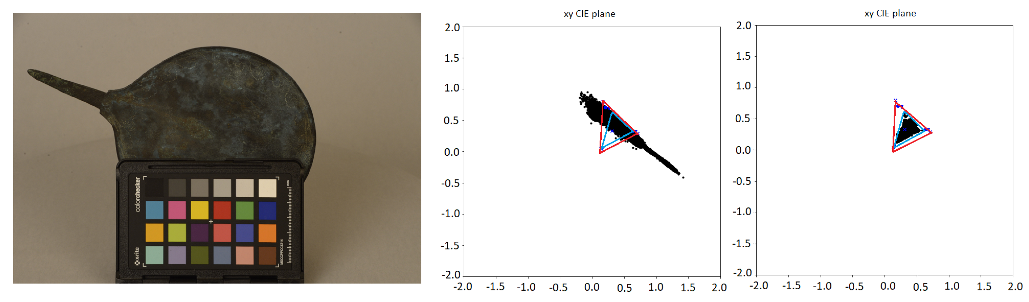
3.2. Colour Calibration
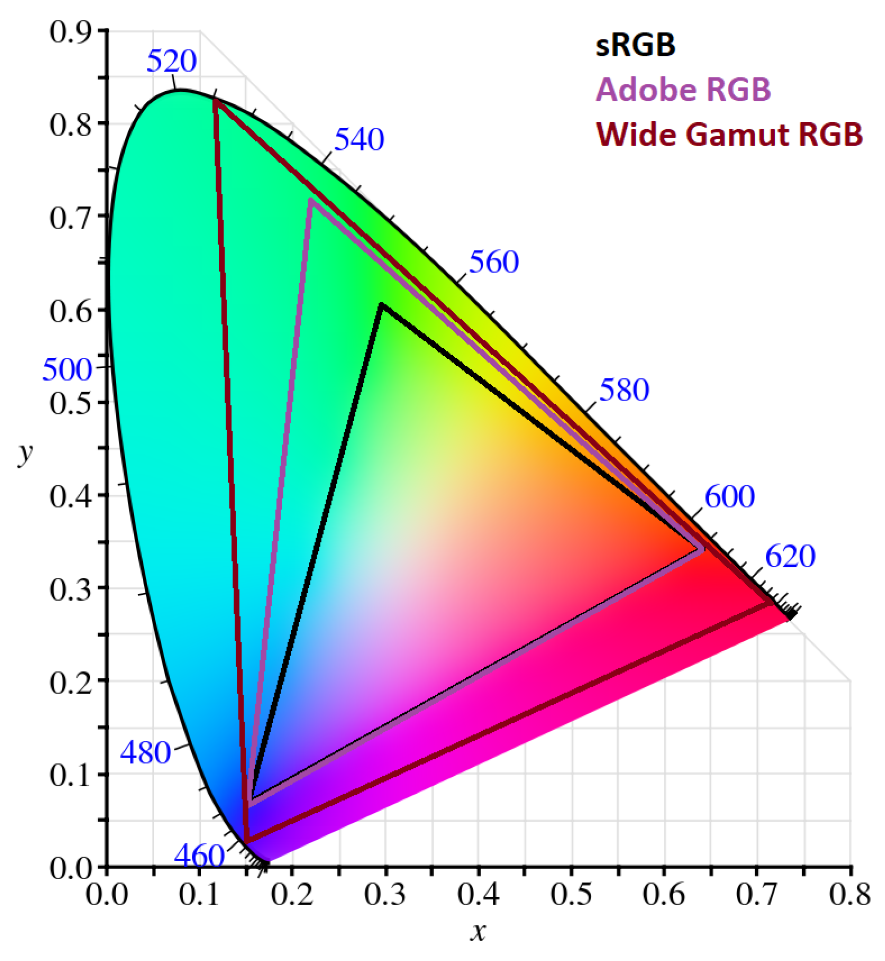
- A digital RGB space is defined by its R, G, and B primaries, which are specified in its documentation. These serve effectively as limits to the gamut. When defining the limits of the space, all its domain can be calibrated without the need to extrapolate colour values. This is important to know, considering that a colour calibration consists fundamentally in algebraic displacements, resizing and interpolations in the operational colour space with a reference to reach. This references—a set of colours sparse in space—can be achieved. Camera RGB values calculated from raw data lack these standardized primaries, so operating with them is tedious for disjoint sources.
- Camera RGB values are direct translations from the perceived light stimuli, which do not always have to correspond to the concrete colours defined within the CIE plane and solid. Transformation into a standardized digital RGB does not only ensure that all colours depicted can be accepted by presentation devices, but also ensures the correct perception of visual information, which is ultimately a mandatory condition when dealing with content sensed by human eyes.
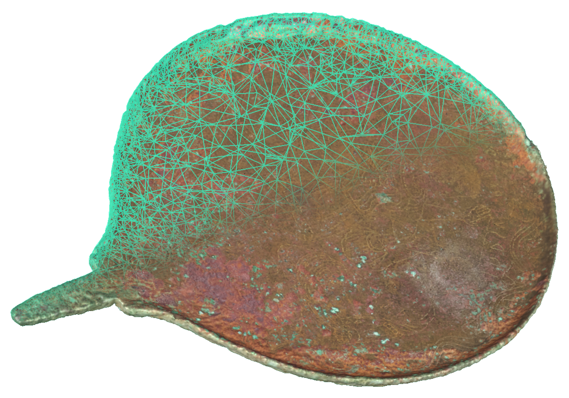
3.3. Photogrammetry
3.4. Evaluation
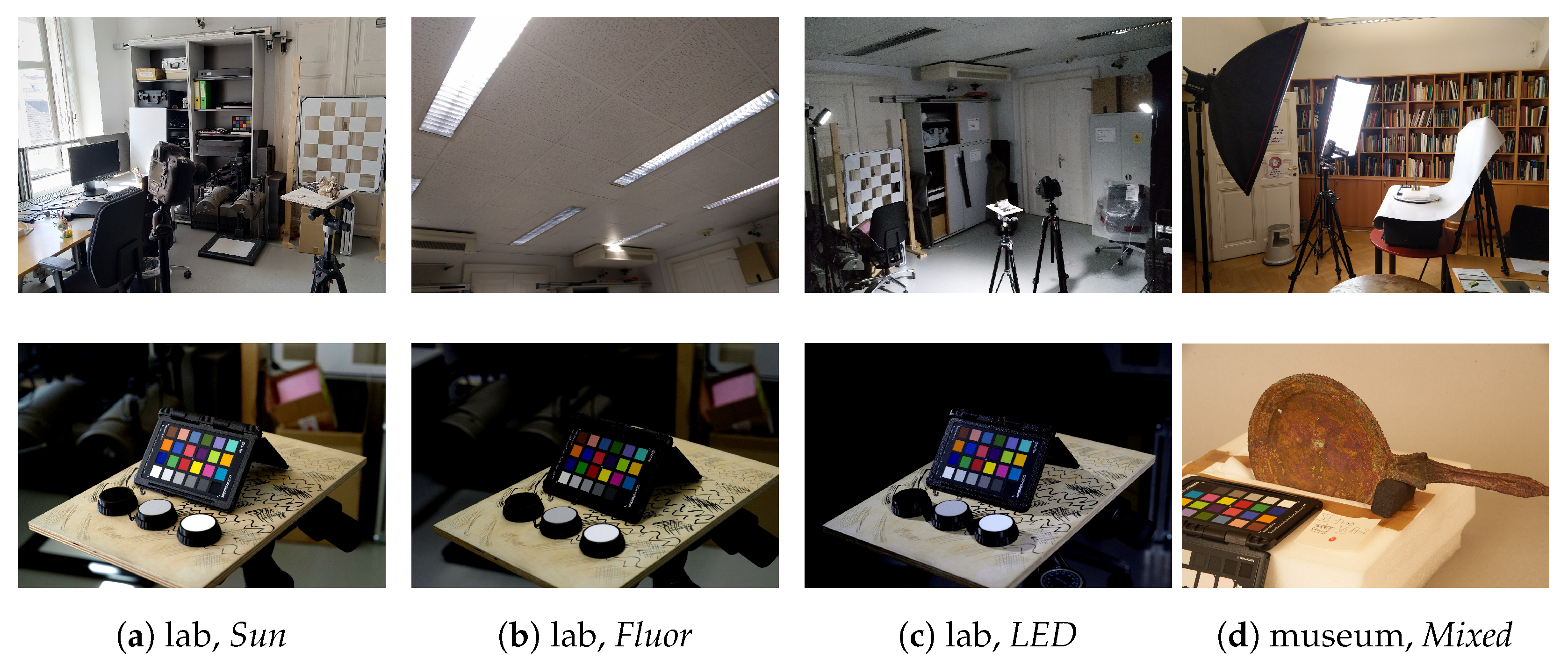
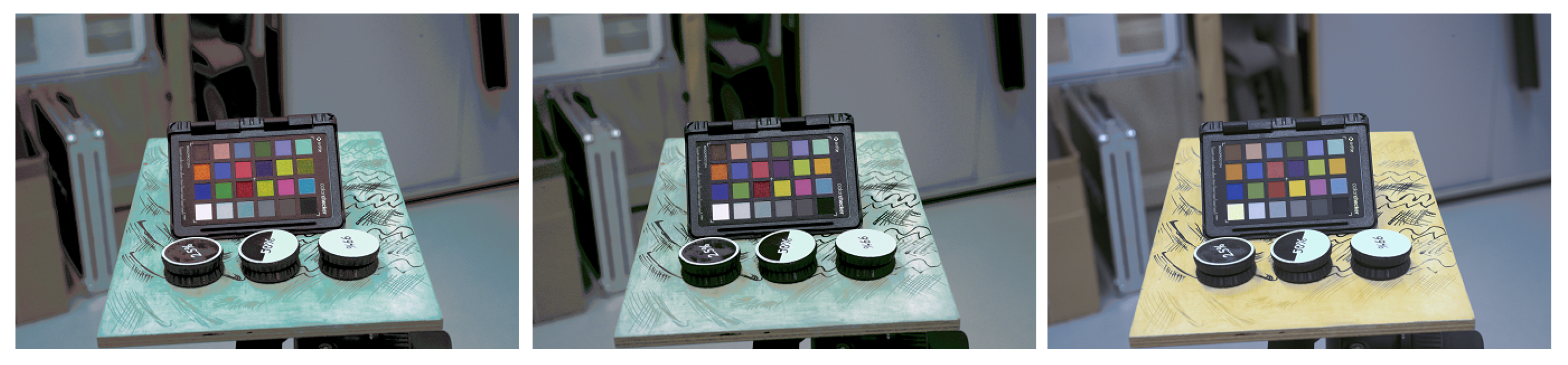
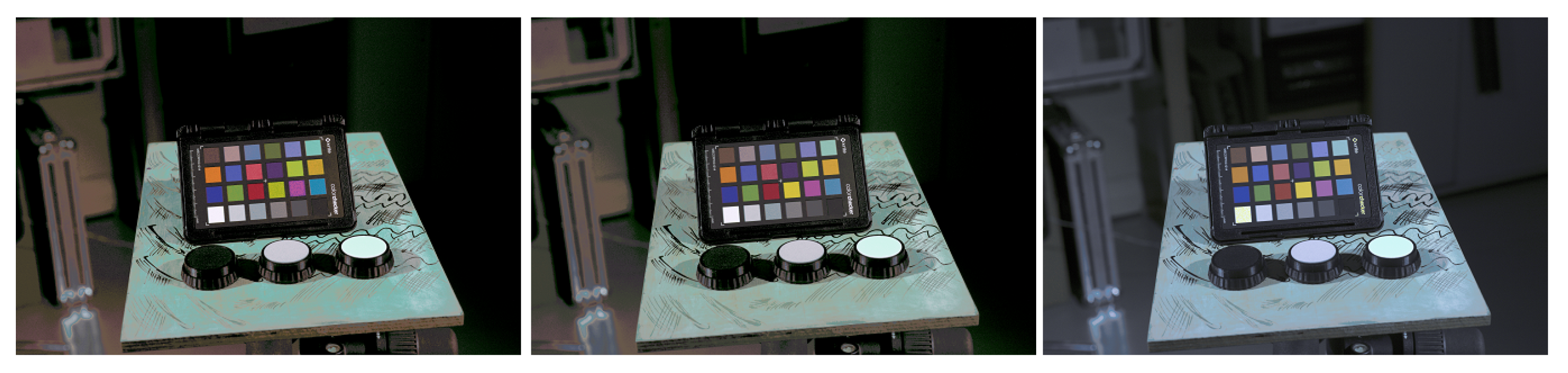
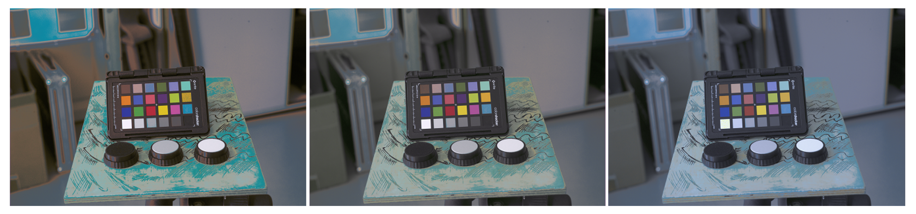
4. Experiments
- Indirect sunlight—“Sun” set: Imaging took place on a sunny afternoon (10 August 2022, between 14:48 and 14:58), with two large windows facing south-west opened. The sunlight did not directly fall on the imaged objects.
- Fluorescent room light—“Fluor” set: The aforementioned windows were closed and covered with black cloth; light was provided by an array of conventional fluorescent lights installed on the ceiling.
- White LEDs—“LED” set: Two Lightpanels MicroPro were mounted on tripods on opposite sides of the object, in an elevation angle of approximately 45.
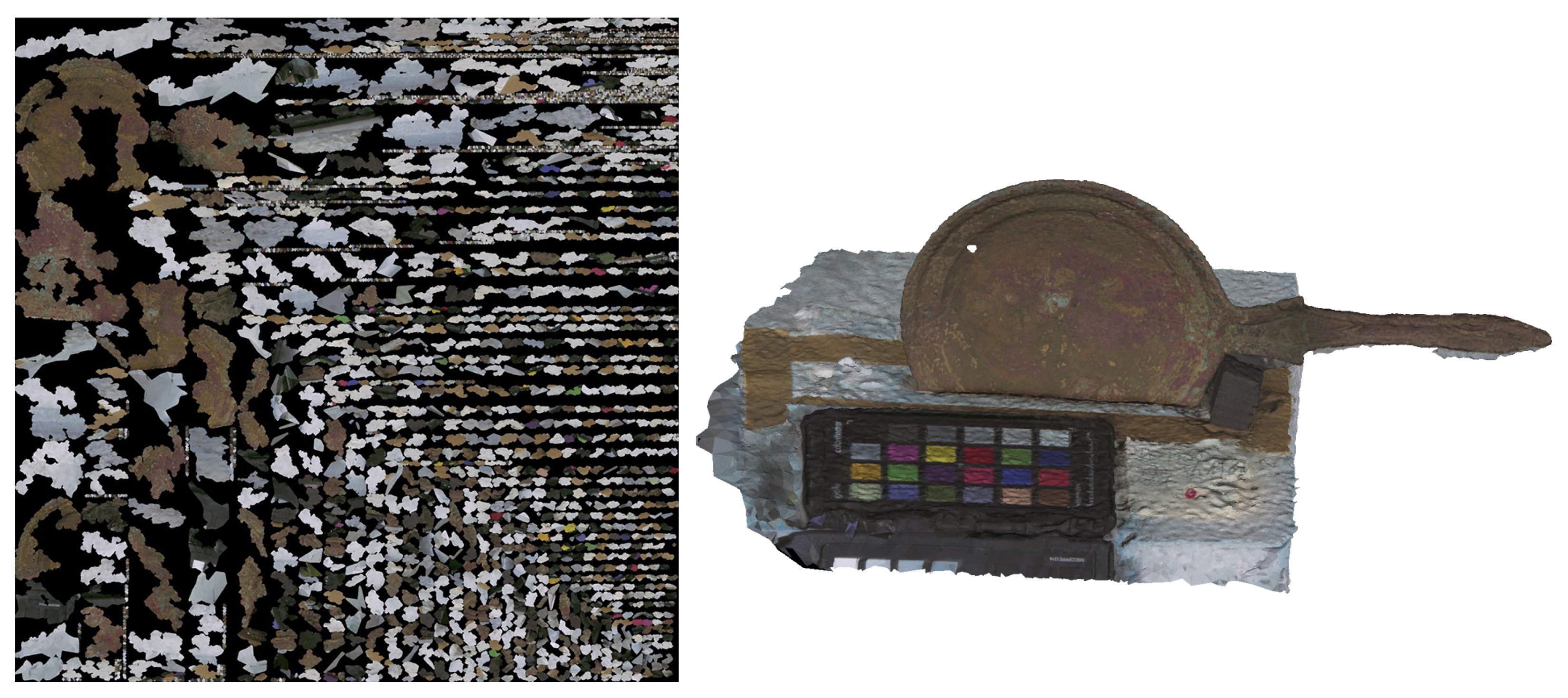
5. Results
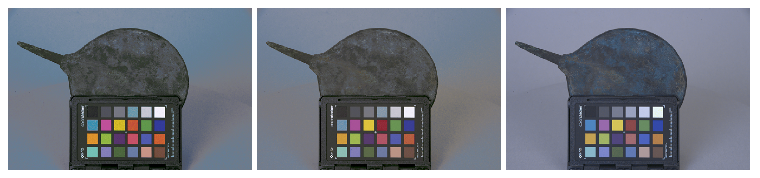
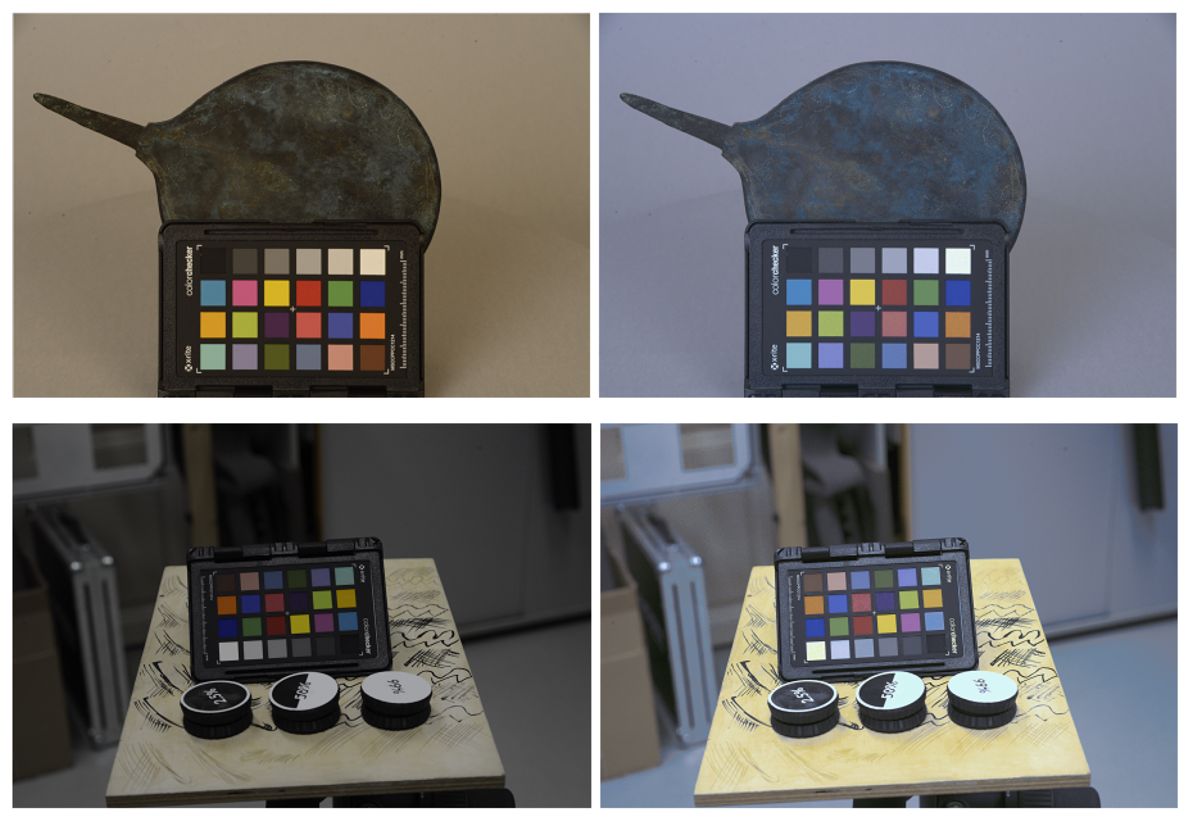
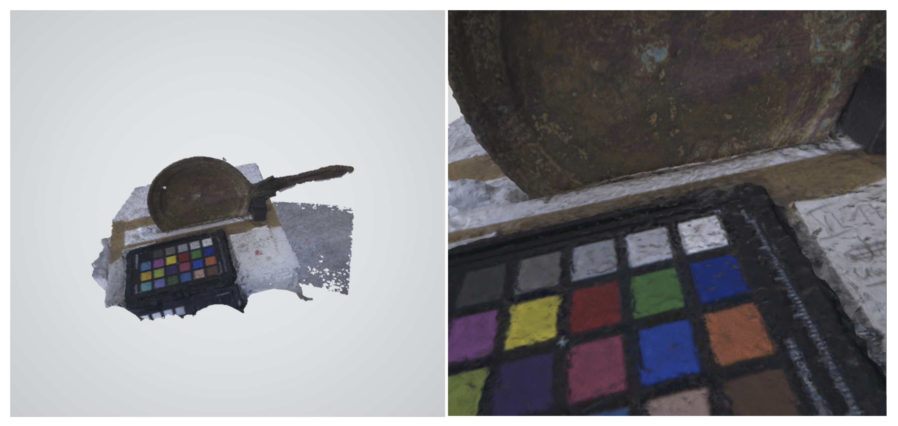
5.1. Visual Inspection
5.2. Quality Metric Analysis
6. Conclusions
Supplementary Materials
Author Contributions
Funding
Conflicts of Interest
| 1 | This work was performed within the project “Etruscan Mirrors in Austria (EtMirA)”, Austrian Science Fund, grant no. P 33721-G. |
References
- Arnold, D. Computer Graphics and Cultural Heritage: From One-Way Inspiration to Symbiosis, Part 1. IEEE Comput. Graph. Appl. 2014, 34, 76–86. [Google Scholar] [CrossRef]
- Torres, J.C.; López, L.; Romo, C.; Arroyo, G.; Cano, P.; Lamolda, F.; Villafranca, M.M. Using a Cultural Heritage Information System for the documentation of the restoration process. In Proceedings of the 2013 Digital Heritage International Congress (DigitalHeritage), Marseille, France, 28 October–1 November 2013; Volume 2, pp. 249–256. [Google Scholar] [CrossRef]
- Nespeca, R. Towards a 3D digital model for management and fruition of Ducal Palace at Urbino. An integrated survey with mobile mapping. SCIRES-IT 2018, 8, 1–14. [Google Scholar] [CrossRef]
- Liyu, F.; Chenchen, H.; Yi, S. Application modes of virtual restoration and reconstruction technology in protection and presentation for cultural heritage in China. In Proceedings of the 2013 Digital Heritage International Congress (DigitalHeritage), Marseille, France, 28 October–1 November 2013; Volume 2, pp. 353–356. [Google Scholar] [CrossRef]
- He, N.; Li, J.; Wang, K.; Guo, L. A Study on the Expression of Jingchu Cultural Heritage. In Proceedings of the 2021 International Conference on Culture-oriented Science & Technology (ICCST), Beijing, China, 18–21 November 2021; pp. 409–412. [Google Scholar] [CrossRef]
- McCarthy, J. Multi-image photogrammetry as a practical tool for cultural heritage survey and community engagement. J. Archaeol. Sci. 2014, 43, 175–185. [Google Scholar] [CrossRef]
- Brown, M.S. Understanding the In-Camera Image Processing Pipeline for Computer Vision; IEEE CVPR 2016; National University of Singapore: Singapore, 2016. [Google Scholar]
- Barbero-Álvarez, M.A.; Rodrigo, J.A.; Menéndez, J.M. Self-Designed Colour Chart and a Multi-Dimensional Calibration Approach for Cultural Heritage Preventive Preservation. IEEE Access 2021, 9, 138371–138384. [Google Scholar] [CrossRef]
- Boochs, F.; Bentkowska-Kafel, A.; Degrigny, C.; Karaszewski, M.; Karmacharya, A.; Kato, Z.; Marcello, P.; Sitnik, R.; Treméau, A.; Tsiafaki, D.; et al. Colour and Space in Cultural Heritage: Interdisciplinary Approaches to Documentation of Material Culture. Int. J. Herit. Digit. Era 2014, 3, 713–730. [Google Scholar] [CrossRef]
- Russ, J.C.; Neal, F.B. The Image Processing Handbook, 7th ed.; CRC Press, Inc.: Boca Raton, FL, USA, 2015. [Google Scholar]
- Emmel, P.; Hersch, R. Colour calibration for colour reproduction. In Proceedings of the 2000 IEEE International Symposium on Circuits and Systems (ISCAS), Geneva, Switzerland, 28–31 May 2000; Volume 5, pp. 105–108. [Google Scholar] [CrossRef] [Green Version]
- Ohta, N. Colorimetry, Fundamentals and Applications; Wiley–IST Series in Imaging Science and Technology; John Wiley and Sons, Ltd.: Hoboken, NJ, USA, 2005. [Google Scholar]
- Bandara, R. A Music Keyboard with Gesture Controlled Effects Based on Computer Vision. Ph.D. Thesis, University of Sri Jayewardenepura, Nugegoda, Sri Lanka, 2011. [Google Scholar]
- Canon. White Paper New Generation 2/3-inch 4K UHD Long Zoom EFP Lenses; Canon Europe: Hillingdon, UK, 2017. [Google Scholar]
- Park, H.W.; Choi, J.W.; Choi, J.Y.; Joo, K.K.; Kim, N.R. Investigation of the Hue-Wavelength Response of a CMOS RGB-Based Image Sensor. Sensors 2022, 22, 9497. [Google Scholar] [CrossRef] [PubMed]
- Dong, X.; Xu, W.; Miao, Z.; Ma, L.; Zhang, C.; Yang, J.; Jin, Z.; Teoh, A.B.J.; Shen, J. Abandoning the Bayer-Filter to See in the Dark. arXiv 2022, arXiv:2203.04042. [Google Scholar]
- Johnston-Feller, R. Color Science in the Examination of Museum Objects: Nondestructive Procedures; Getty Publications: Los Angeles, CA, USA, 2001. [Google Scholar]
- Molada, A.; Marqués-Mateu, A.; Lerma, J. Correct use of color for Cultural Heritage documentation. ISPRS Ann. Photogramm. Remote Sens. Spat. Inf. Sci. 2019, IV-2/W6, 107–113. [Google Scholar] [CrossRef] [Green Version]
- Wang, K.A.; Liao, Y.C.; Tsai, M.T.; Chan, P.C. Research and Practice of Cultural Heritage Promotion: The Case Study of Value Add Application for Folklore Artifacts. In Proceedings of the 2012 International Symposium on Computer, Consumer and Control, Taichung, Taiwan, 4–6 June 2012; pp. 610–613. [Google Scholar] [CrossRef]
- Sun, W.; Li, H.G.; Xu, X. Research on Key Technologies of Three-dimensional Digital Reconstruction of Cultural Heritage in Historical and Cultural Blocks. In Proceedings of the 2021 International Conference on Computer Technology and Media Convergence Design (CTMCD), Sanya, China, 23–25 April 2021; pp. 222–226. [Google Scholar] [CrossRef]
- Karaszewski, M.; Lech, K.; Bunsch, E.; Sitnik, R. In the Pursuit of Perfect 3D Digitization of Surfaces of Paintings: Geometry and Color Optimization. In Proceedings of the Digital Heritage. Progress in Cultural Heritage: Documentation, Preservation, and Protection, Limassol, Cyprus, 3–8 November 2014; Ioannides, M., Magnenat-Thalmann, N., Fink, E., Žarnić, R., Yen, A.Y., Quak, E., Eds.; Springer International Publishing: Cham, Switzerland, 2014; pp. 25–34. [Google Scholar]
- RawPy. RawPy-API. 2023. Available online: https://letmaik.github.io/rawpy/api/ (accessed on 2 July 2023).
- Hirakawa, K.; Parks, T. Adaptive Homogeneity-Directed Demosaicing Algorithm. IEEE Trans. Image Process. 2005, 14, 360–369. [Google Scholar] [CrossRef] [PubMed]
- Griwodz, C.; Gasparini, S.; Calvet, L.; Gurdjos, P.; Castan, F.; Maujean, B.; Lillo, G.D.; Lanthony, Y. AliceVision Meshroom: An open-source 3D reconstruction pipeline. In Proceedings of the 12th ACM Multimedia Systems Conference, MMSys’21, Istanbul, Turkey, 28 September–1 October 2021; ACM Press: New York, NY, USA, 2021. [Google Scholar] [CrossRef]
- Burt, P.J.; Adelson, E.H. A Multiresolution Spline with Application to Image Mosaics. ACM Trans. Graph. 1983, 2, 217–236. [Google Scholar] [CrossRef]
- Lévy, B.; Petitjean, S.; Ray, N.; Maillot, J. Least Squares Conformal Maps for Automatic Texture Atlas Generation. ACM Trans. Graph. 2002, 21, 362–371. [Google Scholar] [CrossRef]
- Luo, M.; Cui, G.; Rigg, B. The development of the CIE 2000 colour-difference formula: CIEDE2000. Color Res. Appl. 2001, 26, 340–350. [Google Scholar] [CrossRef]
- ITU-Ra. Recommendation ITU-R BT.709-6. 2015. Available online: https://www.itu.int/dms_pubrec/itu-r/rec/bt/R-REC-BT.709-6-201506-I!!PDF-E.pdf (accessed on 2 July 2023).
- Adobe. Adobe RGB (1998) Color Image Encoding. 2005. Available online: https://www.adobe.com/digitalimag/adobergb.html (accessed on 2 July 2023).
- Pascale, D. A Review of RGB Color Spaces. 2003. Available online: https://babelcolor.com/index_htm_files/A%20review%20of%20RGB%20color%20spaces.pdf (accessed on 2 July 2023).
- Barbero-Álvarez, M.A.; Menéndez, J.M.; Rodrigo, J.A. An Adaptive Colour Calibration for Crowdsourced Images in Heritage Preservation Science. IEEE Access 2020, 8, 185093–185111. [Google Scholar] [CrossRef]


| List of Primary Chromaticity Coordinates for Different RGB Digitalisations | ||||||||
|---|---|---|---|---|---|---|---|---|
| Space | R Primary | G Primary | B Primary | Reference White | ||||
| x | y | x | y | x | y | x | y | |
| sRGB | 0.64 | 0.33 | 0.3 | 0.6 | 0.15 | 0.06 | 0.3127 | 0.329 |
| Adobe RGB | 0.64 | 0.33 | 0.21 | 0.71 | 0.15 | 0.06 | 0.314 | 0.351 |
| Wide RGB | 0.73 | 0.27 | 0.12 | 0.83 | 0.15 | 0.02 | 0.3457 | 0.3585 |
| Setup ID | Sun | Fluor | LED | Mixed |
|---|---|---|---|---|
| Environment | laboratory | museum | ||
| Lighting | indirect sunlight | fluorescent room light | white LED | 2x halogen softboxes +fluorescent room light |
| Acquisition mode | moving camera | turntable | ||
| Lens | Nikkor | Tamron | ||
| Aperture | f/10 | f/16 | ||
| ISO | 500 | 640 | 640 | 1000 |
| Exposure | 1/40 | 1/30 | 1/10 | 1/60 s |
| Discard | Discard | Interp. | Interp. | Direct | Direct | |
|---|---|---|---|---|---|---|
| Metric | -D50 | -D65 | -D50 | -D65 | -D50 | -D65 |
| Mixed-Adobe | 12.422 | 12.728 | 12.157 | 12.366 | 12.279 | 12.483 |
| Mixed-sRGB | 12.743 | 13.034 | 12.962 | 13.276 | 14.284 | 14.514 |
| Mixed-Wide | 11.313 | 11.296 | 11.237 | 11.247 | 11.033 | 11.049 |
| Fluor-Adobe | 4.207 | 4.648 | 4.215 | 4.640 | 4.610 | 4.861 |
| Fluor-sRGB | 5.242 | 5.493 | 5.344 | 5.562 | 8.420 | 8.441 |
| Fluor-Wide | 4.584 | 4.765 | 4.524 | 4.671 | 4.332 | 4.380 |
| LED-Adobe | 6.175 | 6.154 | 5.974 | 6.001 | 6.440 | 6.512 |
| LED-sRGB | 6.352 | 6.274 | 6.220 | 6.120 | 6.314 | 6.220 |
| LED-Wide | 5.723 | 5.518 | 5.480 | 5.331 | 5.982 | 5.822 |
| Sun-Adobe | 8.592 | 8.820 | 8.968 | 9.279 | 10.574 | 10.980 |
| Sun-sRGB | 8.640 | 9.051 | 9.538 | 9.845 | 13.525 | 13.640 |
| Sun-Wide | 8.109 | 8.230 | 8.127 | 8.411 | 8.849 | 8.961 |
| Discard | Discard | Interp. | Interp. | Direct | Direct | |
|---|---|---|---|---|---|---|
| Metric | -D50 | -D65 | -D50 | -D65 | -D50 | -D65 |
| Mixed-Adobe | 5.831 | 5.914 | 5.816 | 5.864 | 4.248 | 4.272 |
| Mixed-sRGB | 4.990 | 5.623 | 4.906 | 5.664 | 4.811 | 5.381 |
| Mixed-Wide | 4.381 | 4.291 | 4.229 | 4.146 | 4.086 | 4.022 |
| Fluor-Adobe | 2.246 | 2.956 | 2.457 | 3.285 | 2.840 | 3.139 |
| Fluor-sRGB | 2.452 | 2.686 | 3.127 | 3.380 | 12.043 | 11.061 |
| Fluor-Wide | 2.597 | 2.591 | 2.900 | 2.928 | 3.034 | 2.668 |
| LED-Adobe | 2.825 | 2.80 | 3.169 | 3.288 | 2.692 | 3.014 |
| LED-sRGB | 3.182 | 3.032 | 3.320 | 2.960 | 2.734 | 2.604 |
| LED-Wide | 2.226 | 1.795 | 2.265 | 1.978 | 2.255 | 2.006 |
| Sun-Adobe | 4.338 | 4.582 | 4.286 | 4.341 | 6.745 | 7.635 |
| Sun-sRGB | 4.218 | 4.271 | 4.263 | 4.421 | 12.462 | 11.751 |
| Sun-Wide | 4.987 | 4.882 | 4.858 | 4.905 | 5.054 | 4.802 |
Disclaimer/Publisher’s Note: The statements, opinions and data contained in all publications are solely those of the individual author(s) and contributor(s) and not of MDPI and/or the editor(s). MDPI and/or the editor(s) disclaim responsibility for any injury to people or property resulting from any ideas, methods, instructions or products referred to in the content. |
© 2023 by the authors. Licensee MDPI, Basel, Switzerland. This article is an open access article distributed under the terms and conditions of the Creative Commons Attribution (CC BY) license (https://creativecommons.org/licenses/by/4.0/).
Share and Cite
Barbero-Álvarez, M.A.; Brenner, S.; Sablatnig, R.; Menéndez, J.M. Preserving Colour Fidelity in Photogrammetry—An Empirically Grounded Study and Workflow for Cultural Heritage Preservation. Heritage 2023, 6, 5700-5718. https://doi.org/10.3390/heritage6080300
Barbero-Álvarez MA, Brenner S, Sablatnig R, Menéndez JM. Preserving Colour Fidelity in Photogrammetry—An Empirically Grounded Study and Workflow for Cultural Heritage Preservation. Heritage. 2023; 6(8):5700-5718. https://doi.org/10.3390/heritage6080300
Chicago/Turabian StyleBarbero-Álvarez, Miguel Antonio, Simon Brenner, Robert Sablatnig, and José Manuel Menéndez. 2023. "Preserving Colour Fidelity in Photogrammetry—An Empirically Grounded Study and Workflow for Cultural Heritage Preservation" Heritage 6, no. 8: 5700-5718. https://doi.org/10.3390/heritage6080300