
Mass-Transfer Air Pollution Modeling in Heritage Buildings

Abstract
:1. Introduction
2. Indoor Air Pollution Models
2.1. Mass-Balance at Steady-State
2.2. Indoor-Outdoor Ratio (I/O)
2.3. Indoor Air Pollution (IAP)
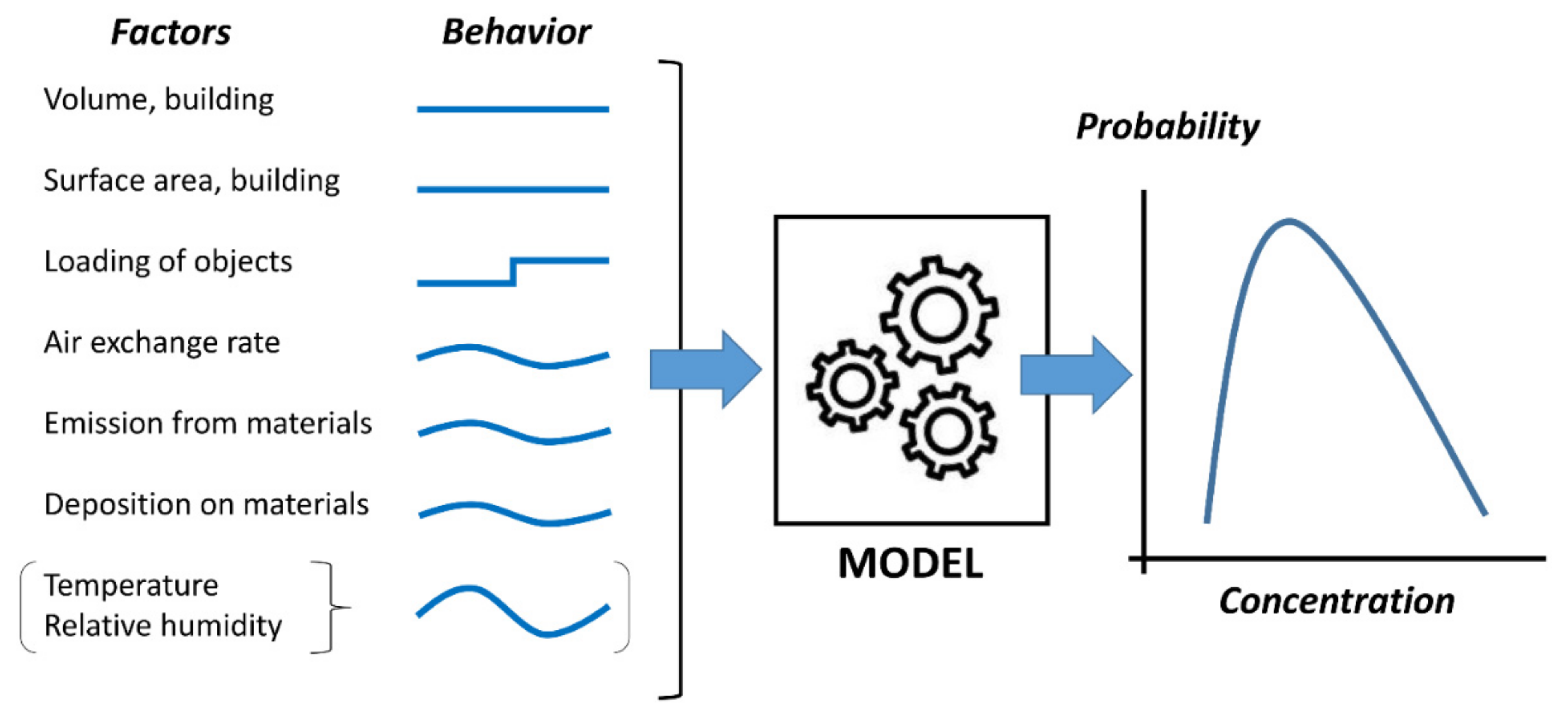
2.4. Monte Carlo Simulations
2.5. Other Computational Simulations
3. Case Study
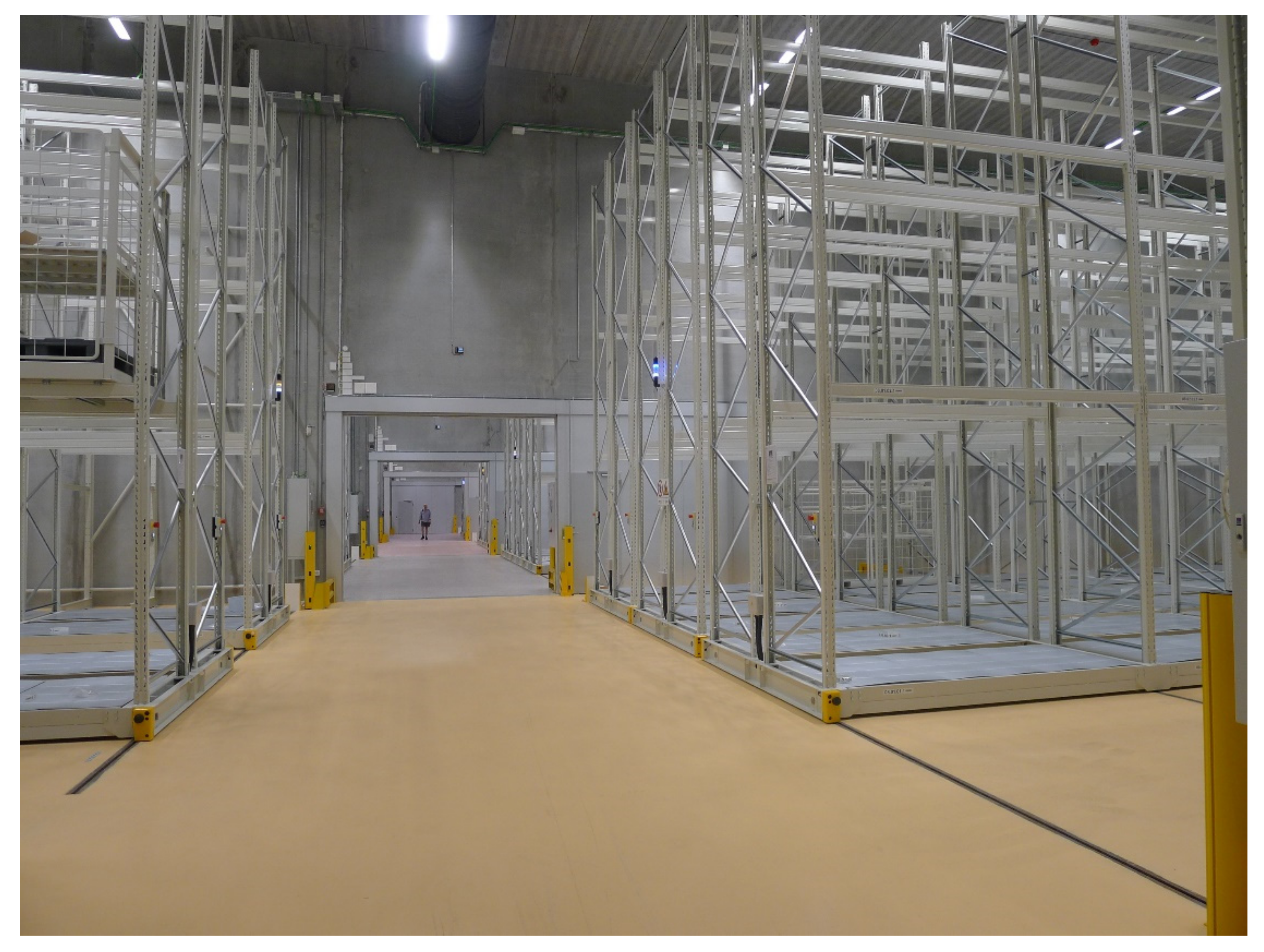
3.1. The National Museum Storage Facility
3.2. The Building
3.3. Ambient Conditions
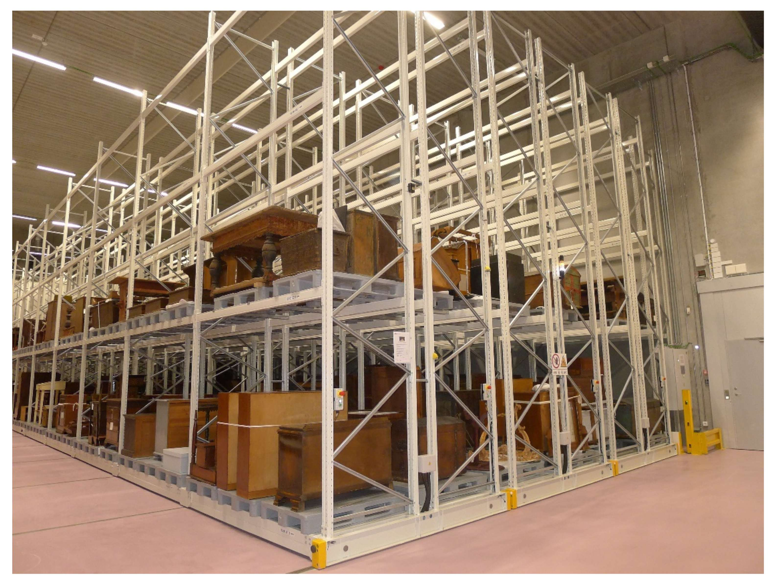
3.4. Collection and Interior
4. Methods
4.1. I/O Model
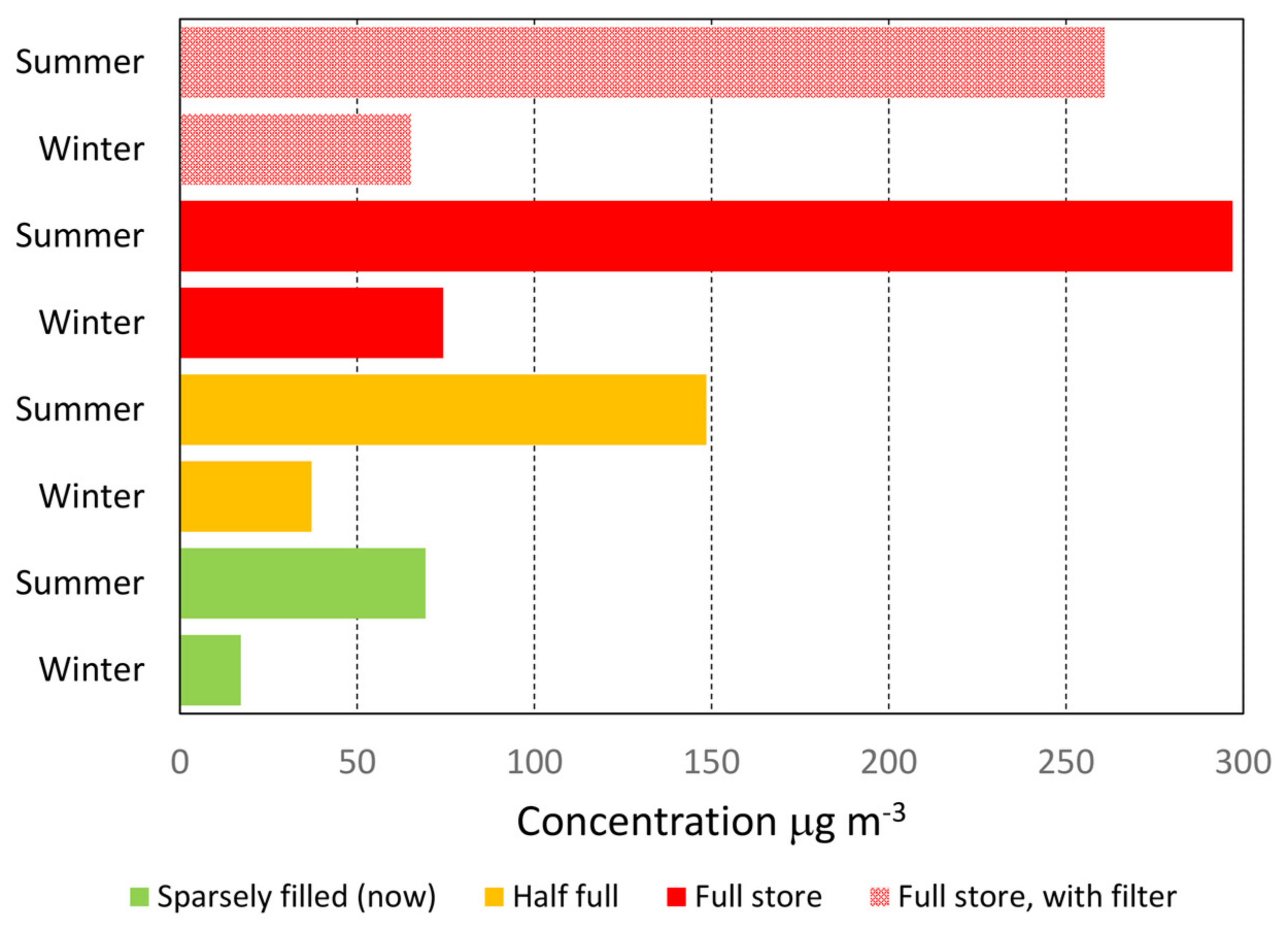
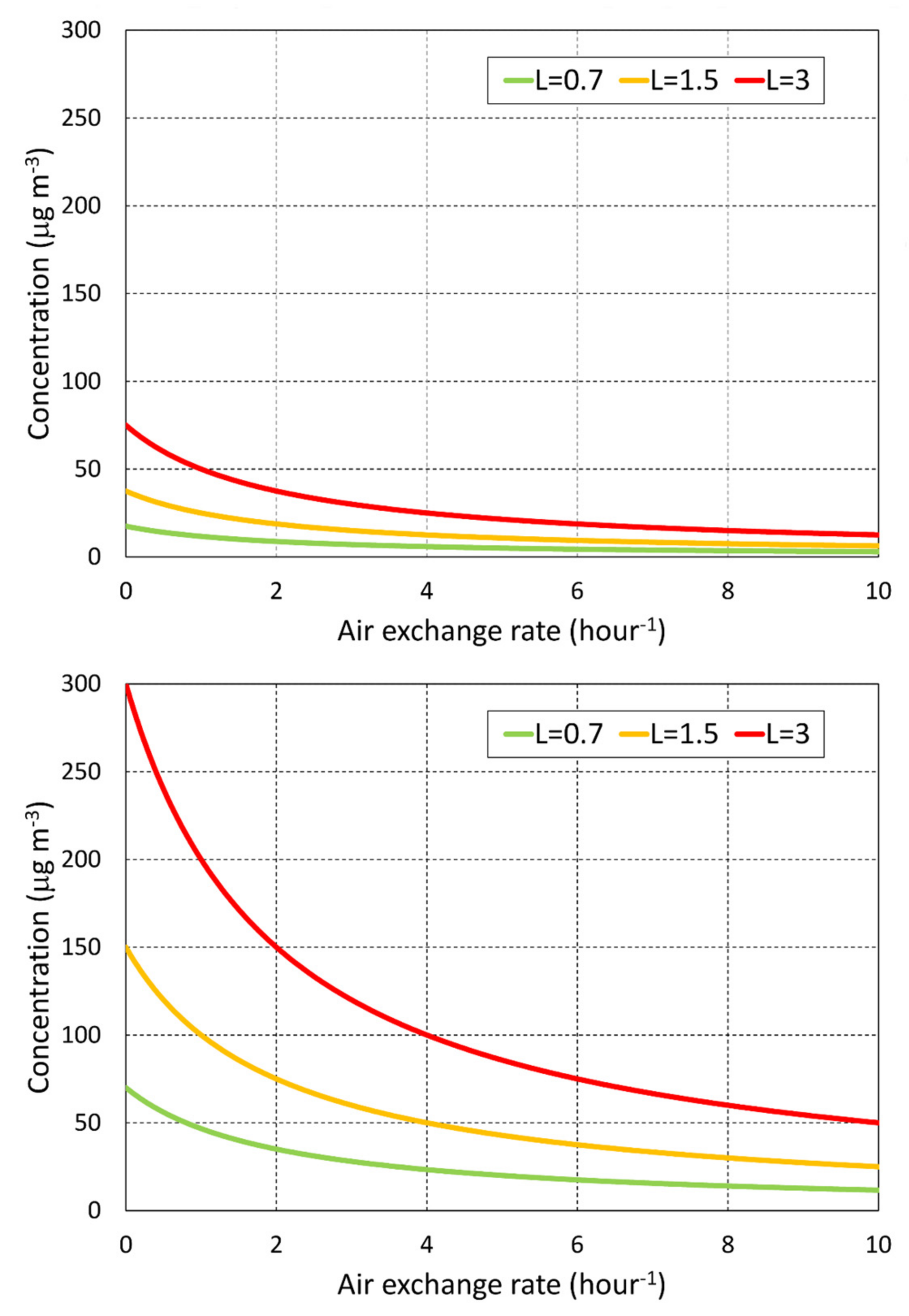
4.2. IAP Model
- Sparsely filled with museum objects (as today) at a loading (L) of 0.7 m2 m−3
- Half-filled storage at L = 1.5 m2 m−3
- Full storage at L = 3 m2 m−3.
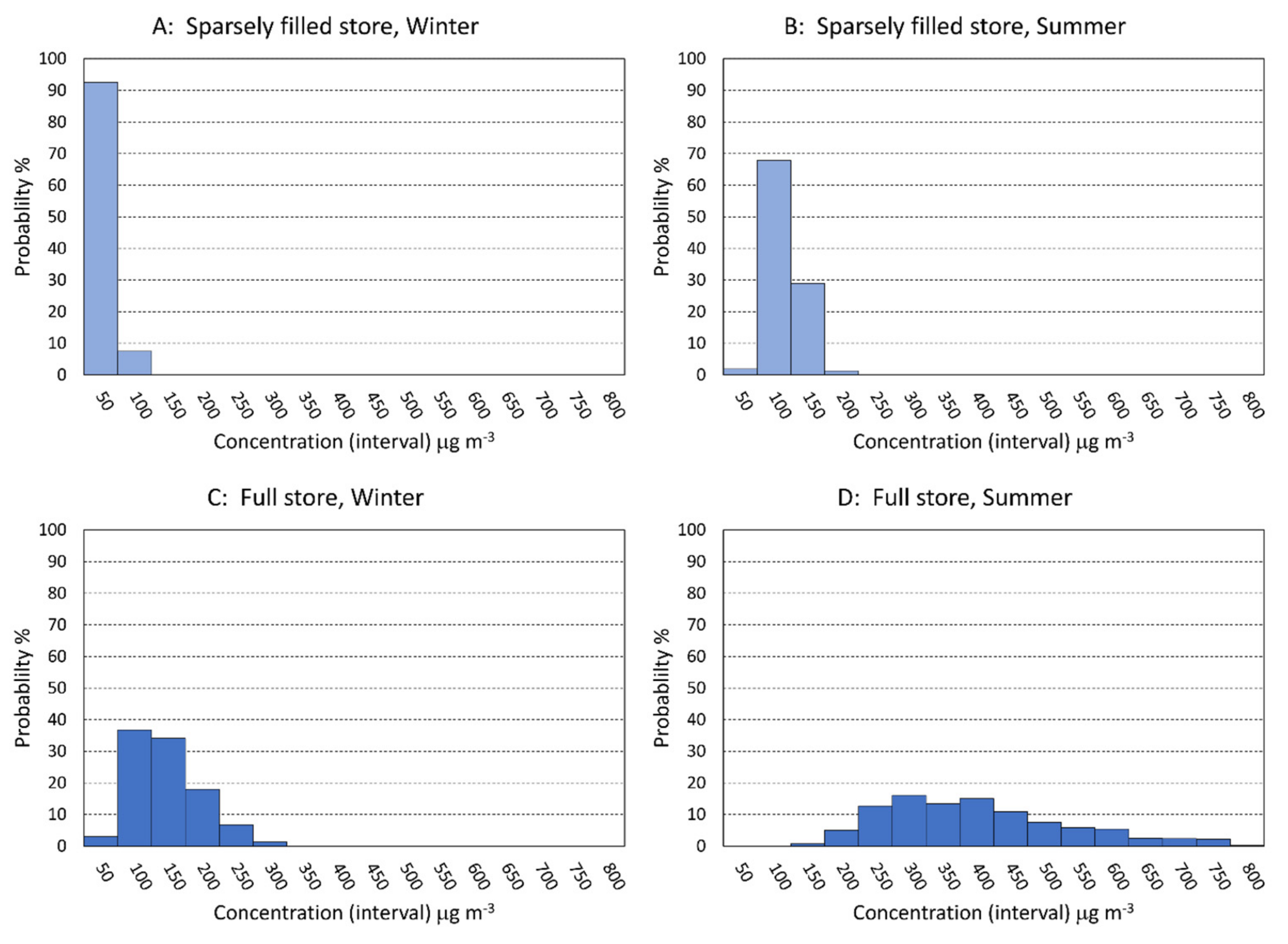
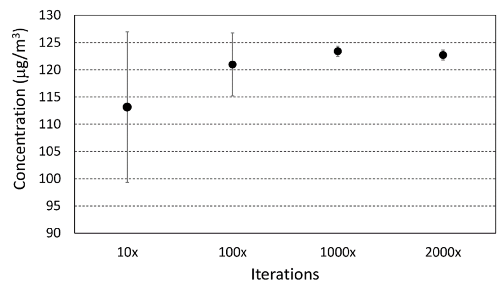
4.3. Monte Carlo Simulation
- Storage hall as now, sparsely loaded with objects, winter temperature.
- Storage hall as now, sparsely loaded with objects, summer temperature.
- Storage hall at full capacity, filled with objects, winter temperature.
- Storage hall at full capacity, filled with objects, summer temperature.
4.4. Pollution Measurements at Site
5. Results
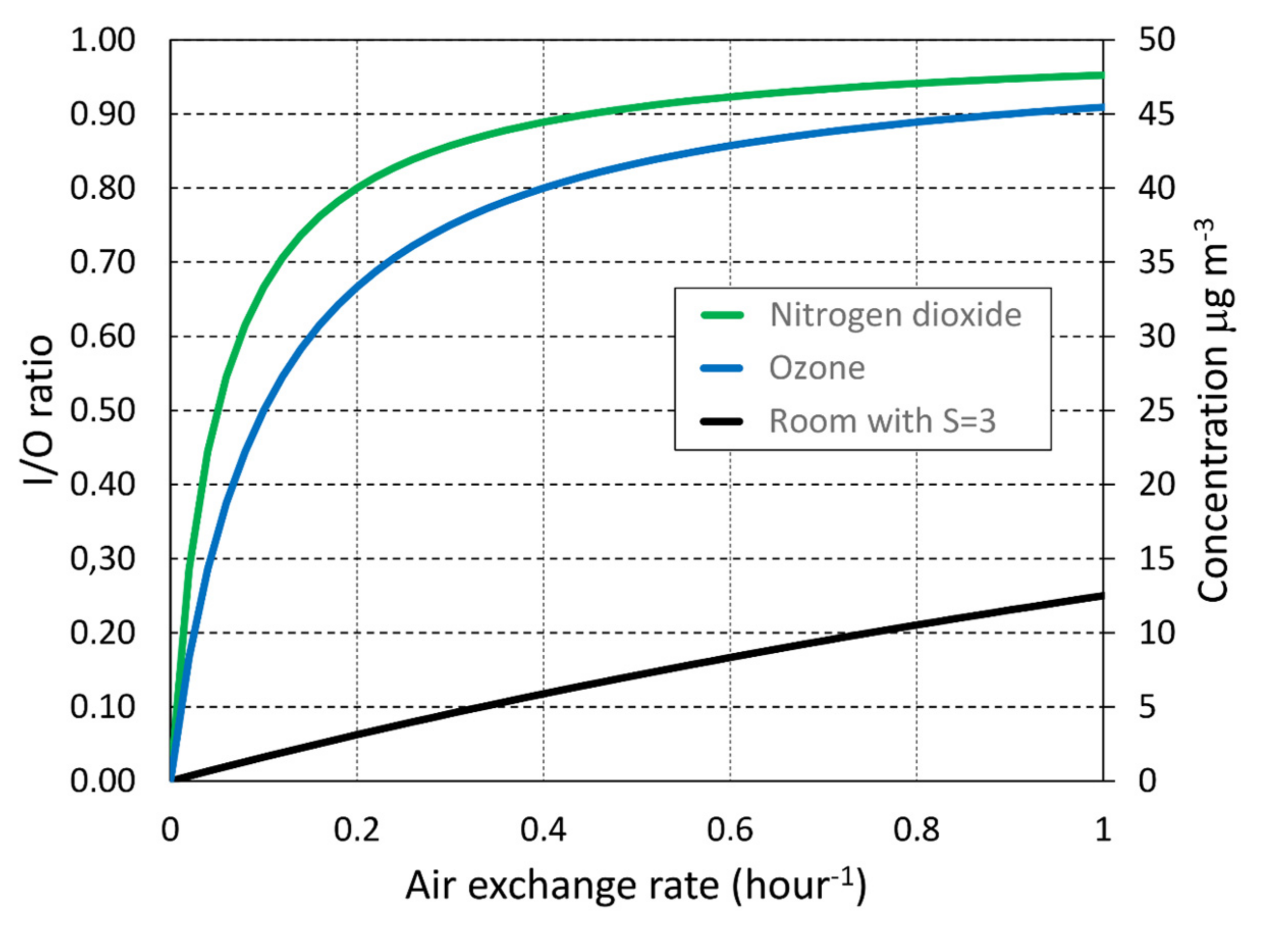
5.1. I/O Model Results
5.2. IAP Model Results
5.3. Monte Carlo Simulation Results
5.4. Pollution Measurements
6. Discussion and Conclusions
6.1. Background Measurements
6.2. Outdoor Pollutants
6.3. Indoor-Generated Pollutants
6.4. Constant versus Dynamic Conditions
6.5. Practical Implications and Perspectives
Author Contributions
Funding
Data Availability Statement
Acknowledgments
Conflicts of Interest
References
- Baer, N.S.; Banks, P.N. Indoor air pollution: Effects on cultural and historic materials. Int. J. Mus. Manag. Curatorship 1985, 4, 9–20. [Google Scholar]
- Brimblecombe, P. The composition of museum atmospheres. Atmos. Environ. Part B Urban Atmos. 1990, 24B, 1–8. [Google Scholar] [CrossRef]
- Graedel, T.E.; McGill, R. Degradation of materials in the atmosphere. Environ. Sci. Technol. 1986, 20, 1093–1100. [Google Scholar] [CrossRef]
- Blades, N.; Oreszczyn, T.; Bordass, B.; Cassar, M. Guidelines on Pollution Control in Museum Buildings; Museums Association: London, UK, 2000. [Google Scholar]
- Hatchfield, P. Pollutants in the Museum Environment-Practical Strategies for Problem Solving in Design, Exhibition and Storage; Archetype Publications Ltd.: London, UK, 2002. [Google Scholar]
- Tétreault, J. Airborne Pollutants in Museums, Galleries and Archives: Risk Assessment, Control Strategies and Preservation Management; Canadian Conservation Institute: Ottawa, ON, Canada, 2003. [Google Scholar]
- Paterakis, A.B. Volatile Organic Compounds and the Conservation of Inorganic Materials; Archetype Publications Ltd.: London, UK, 2016. [Google Scholar]
- Gray, V.R. The Acidity of Wood. J. Wood Sci. 1958, 1, 58–64. [Google Scholar]
- Clarke, S.G.; Longhurst, E.E. The Corrosion of Metals by Acid Vapours from Wood. J. Appl. Chem. 1961, 11, 435–443. [Google Scholar] [CrossRef]
- Smedemark, S.H.; Ryhl-Svendsen, M.; Schieweck, A. Quantification of formic acid and acetic acid emissions from heritage collections under indoor room conditions. Part I: Laboratory and field measurements. Herit. Sci. 2020, 8, 58. [Google Scholar] [CrossRef]
- Smedemark, S.H. The dynamics and control of indoor air pollution in repositories without mechanical ventilation for cultural heritage collections. A literature review. e-Preservation Sci. 2018, 15, 17–29. [Google Scholar]
- Grzywacz, C.M. Using Passive Sampling Devices to Detect Pollutants in Museum Environments. In ICOM Committee for Conservation, Proceedings of the 10th Triennial Meeting, Washington, DC, USA, 22–27 August 1993; Bridgland, J., Ed.; James & James: London, UK, 1993; pp. 610–615. [Google Scholar]
- Ryhl-Svendsen, M.; Smedemark, S.H. Environmental conditions for Danish storage buildings: Reviewing 20 years of air quality surveys. Stud. Conserv. 2023. (submitted). [Google Scholar]
- Ryhl-Svendsen, M. Indoor air pollution in museums: Prediction models and control strategies. Stud. Conserv. 2006, 51 (Suppl. S1), 27–41. [Google Scholar] [CrossRef]
- Dabanlis, G.; Loupa, G.; Tsalidis, G.A.; Kostenidou, E.; Rapsomanikis, S. The Interplay between Air Quality and Energy Efficiency in Museums, a Review. Appl. Sci. 2023, 13, 5535. [Google Scholar] [CrossRef]
- ASHRAE. Museums, Galleries, Archives, and Libraries. In ASHRAE Handbook-HVAC Applications; American Society of Heating, Refrigerating and Air-Conditioning Engineers: Atlanta, GA, USA, 2019; Chapter 24. [Google Scholar]
- Grzywacz, C.M. Monitoring for Gaseous Pollutants in Museum Environments; (Tools for Conservation); The Getty Conservation Institute: Los Angeles, CA, USA, 2006. [Google Scholar]
- Brimblecombe, P. The balance of environmental factors attacking artifacts. In Durability and Change. The Science, Responsibility, and Cost of Sustaining Cultural Heritage. Dahlem Workshop, Berlin, Germany, 1992; Krumbein, W.E., Brimblecombe, P., Cosgrove, D.E., Staniforth, S., Eds.; John Wiley & Sons: New York, NY, USA, 1994; pp. 67–79. [Google Scholar]
- Brimblecombe, P. Pollution Studies. In ENVIRONMENT Leather Project Deterioration and Conservation of Vegetable Tanned Leather; Larsen, R., Ed.; Protection and Conservation of the European Cultural Heritage, Research Report No. 6 of European Commission; The Royal Danish Academy of Fine Arts: Copenhagen, Denmark, 1996; pp. 25–32. [Google Scholar]
- Abdalla, T.E.; Peng, C. Evaluation of housing stock indoor air quality models: A review of data requirements and model performance. J. Build. Eng. 2021, 43, 102846. [Google Scholar] [CrossRef]
- Pepper, D.W.; Carrington, D. Modeling Indoor Air Pollution; Imperial College Press: London, UK, 2009. [Google Scholar]
- Weschler, C.J.; Shields, H.C.; Naik, D.V. Indoor Ozone Exposures. J. Air Pollut. Control. Assoc. 1989, 39, 1562–1568. [Google Scholar] [CrossRef]
- Nazaroff, W.W.; Gadgil, A.J.; Weschler, C.J. Critique of the use of deposition velocity in modeling air quality and exposure. In ASTM Special Technical Publication: Modeling of Indoor Air Quality and Exposure; Nagda, N.L., Ed.; ASTM STP 1205; American Society for Testing and Materials: Philadelphia, PA, USA, 1993; pp. 81–104. [Google Scholar]
- Weschler, C.J. Ozone in indoor environments: Concentration and chemistry. Indoor Air 2000, 10, 269–288. [Google Scholar] [CrossRef] [PubMed] [Green Version]
- Blades, N.; Kruppa, D.; Cassar, M. Development of a web-based software tool for predicting the occurrence and effect of air pollutants inside museum buildings. In ICOM Committee for Conservation, Proceedings of the 13th Triennial Meeting, Rio de Janeiro, Brazil, 22–27 September 2002; Verger, I., Ed.; James & Jamens: London, UK, 2002; pp. 9–14. [Google Scholar]
- Spicer, C.W.; Kenny, D.V.; Ward, G.F.; Billick, I.H. Transformations, Lifetimes, and Sources of NO2, HONO, and HNO3 in Indoor Environments. J. Air Waste Manag. Assoc. 1993, 43, 1479–1485. [Google Scholar] [CrossRef]
- Febo, A.; Perrino, C. Prediction and experimental evidence for high air concentration of nitrous acid in indoor environments. Atmos. Environ. 1991, 25A, 1055–1061. [Google Scholar] [CrossRef]
- Katsanos, N.A.; De Santis, F.; Cordoba, A.; Roubani-Kalantzopoulou, F.; Pasella, D. Corrosive effects from the deposition of gaseous pollutants on surfaces of cultural and artistic value inside museums. J. Hazard. Mater. A 1999, 64, 21–36. [Google Scholar] [CrossRef] [PubMed]
- Brimblecombe, P.; Blades, N.; Camuffo, D.; Sturaro, G.; Valentino, A.; Gysels, K.; Van Grieken, R.; Busse, H.-J.; Kim, O.; Wieser, M. The indoor environment of a modern museum building, The Sainsbury Centre for Visual Arts, Norwich, UK. Indoor Air 1999, 9, 146–164. [Google Scholar] [CrossRef]
- Grøntoft, T.; Raychaudhuri, M.R. Compilation of tables of surface deposition velocities for O3, NO2 and SO2 to a range of indoor surfaces. Atmos. Environ. 2004, 38, 533–544. [Google Scholar] [CrossRef]
- Ryhl-Svendsen, M. The role of air exchange rate and surface reaction rates on the air quality in museum storage buildings. In Museum Microclimates, Proceedings of the Copenhagen Conference, Copenhagen, Denmark, 19–23 November 2007; Padfield, T., Borchersen, K., Eds.; National Museum of Denmark: Copenhagen, Denmark, 2007; pp. 221–226. [Google Scholar]
- Smedemark, S.H.; Ryhl-Svendsen, M. Determining the level of organic acid air pollution in museum storage rooms by mass-balance modelling. J. Cult. Herit. 2022, 55, 309–317. [Google Scholar] [CrossRef]
- McVoy, G.R. Monte Carlo Simulation Techniques Applied to Air Quality Impact Assessment. J. Air Pollut. Control Assoc. 1979, 29, 843–845. [Google Scholar] [CrossRef] [Green Version]
- Johnson, M.; Lam, N.; Brant, S.; Charron, D.; Gray, C.; Pennise, D. Modeling indoor air pollution from cookstove emissions in developing countries using a Monte Carlo single-box model. Atmos. Environ. 2011, 45, 3237–3243. [Google Scholar] [CrossRef]
- Kruza, M.; Shaw, D.; Shaw, J.; Carslaw, N. Towards improved models for indoor air chemistry: A Monte Carlo simulation study. Atmos. Environ. 2021, 262, 118625. [Google Scholar] [CrossRef]
- Dai, X.; Liu, J.; Zhang, X. Monte Carlo simulation to control indoor pollutants from indoor and outdoor sources for residential buildings in Tianjin, China. Build. Eviron. 2019, 165, 106376. [Google Scholar] [CrossRef]
- Weschler, C.J.; Shields, H.C.; Naik, D.V. Indoor chemistry involving O3, NO, and NO2 as evidence by 14 months of measurements at a site in Southern California. Environ. Sci. Technol. 1994, 28, 2120–2132. [Google Scholar] [CrossRef] [PubMed]
- Weschler, C.J.; Shields, H.C. Potential reactions among indoor pollutants. Atmos. Environ. 1997, 31, 3487–3495. [Google Scholar] [CrossRef]
- Nazaroff, W.W.; Cass, G.R. Mathematical modeling of chemically reactive pollutants in indoor air. Environ. Sci. Technol. 1986, 20, 924–934. [Google Scholar] [CrossRef] [Green Version]
- Carslaw, N. A new detailed chemical model for indoor air pollution. Atmos. Environ. 2007, 41, 1164–1179. [Google Scholar] [CrossRef]
- Druzic, J.; Adams, M.; Tiller, C.; Cass, G.R. The measurement and model predictions of indoor ozone concentrations in museums. Atmos. Environ. 1990, 24A, 1813–1823. [Google Scholar] [CrossRef]
- Drakou, G.; Zerefos, C.; Ziomas, I.; Gantis, V. Numerical simulation of indoor air pollution levels in a church and in a museum in Greece. Stud. Conserv. 2000, 45, 85–94. [Google Scholar]
- Pagonis, D.; Price, D.J.; Algrim, L.B.; Day, D.A.; Handschy, A.V.; Stark, H.; Miller, S.L.; de Gouw, J.; Jimenez, J.L.; Ziemann, P.J. Time-resolved measurements of indoor chemical emissions, deposition, and reactions in a university art museum. Environ. Sci. Technol. 2019, 53, 4794–4802. [Google Scholar] [CrossRef]
- Li, Y.; Nielsen, P.V. CFD and ventilation research. Indoor Air 2011, 21, 442–453. [Google Scholar] [CrossRef] [PubMed]
- Grau-Bové, J.; Mazzei, L.; Strlic, M.; Cassar, M. Fluid simulations in heritage science. Herit. Sci. 2019, 7, 16. [Google Scholar] [CrossRef]
- Ascione, F.; Bellia, L.; Capozzoli, A. A coupled numerical approach on museum air conditioning: Energy and fluid-dynamic analysis. Appl. Energy 2013, 103, 416–427. [Google Scholar] [CrossRef]
- Grau-Bové, J.; Strlič, M. Fine particulate matter in indoor cultural heritage: A literature review. Herit. Sci. 2013, 1, 8. [Google Scholar] [CrossRef] [Green Version]
- Mašková, L.; Smolík, J.; Ondráček, J.; Ondráčková, L.; Travnickova, T.; Havlica, J. Air quality in archives housed in historic buildings: Assessment of concentration of indoor particles of outdoor origin. Build. Eviron. 2020, 180, 107024. [Google Scholar] [CrossRef]
- Grau-Bové, J.; Mazzei, L.; Malki-Ephstein, L.; Thickett, D.; Strlič, M. Simulation of particulate matter ingress, dispersion and deposition in a historical building. J. Cult. Herit. 2016, 18, 199–208. [Google Scholar] [CrossRef]
- Camuffo, D. Microclimate for Cultural Heritage: Measurements, Risk Assessment, Conservation, Restoration, and Maintaince of Indoor and Outdoor Monuments, 3rd ed.; Elsevier: Amsterdam, The Netherlands, 2019; pp. 197–234. [Google Scholar]
- Morawska, L.; Salthammer, T. Fundamentals. In Indoor Environment, Airborne Particles and Settled Dust; Morawska, L., Salthammer, T., Eds.; Wiley-WCH Verlag GmbH & Co. KGaA: Weinheim, Germany, 2003; pp. 1–46. [Google Scholar]
- Fællesmagasinet (In Danish: The Joint Storage Facility). Danish Agency for Culture and Palaces. Available online: https://slks.dk/omraader/slotte-og-ejendomme/bygge-og-udviklingsprojekter/faellesmagasinet (accessed on 1 May 2023).
- Janssen, H.; Christensen, J.E. Hygrothermal optimisation of museum storage spaces. Energy Build. 2013, 56, 169–178. [Google Scholar] [CrossRef]
- Ryhl-Svendsen, M.; Jensen, L.A.; Larsen, P.K.; Bøhm, B.; Padfield, T. Ultra-low-energy museum storage. In Proceedings of the ICOM-CC 16th Triennial Conference, Lisbon, Portugal, 19–23 September 2011; Bridgland, J., Ed.; ICOM Committee for Conservation: Paris, France, 2011; p. 8. [Google Scholar]
- Department of Environmental Sciences, Aarhus University. Air Quality Data. Available online: https://envs.au.dk/en/research-areas/air-pollution-emissions-and-effects/air-quality-data (accessed on 1 May 2023).
- Smedemark, S.H.; Ryhl-Svendsen, M. Indoor air pollution in archives: Temperature dependent emission of formic acid and acetic acid from paper. J. Pap. Conserv. 2020, 21, 22–30. [Google Scholar] [CrossRef]
- Ryhl-Svendsen, M.; Jensen, L.A.; Larsen, P.K. Air quality in low-ventilated museum storage buildings. In ICOM Committee for Conservation, Proceedings of the 17th Triennial Conference Preprints, Melbourne, Australia, 15–19 September 2014; Bridgland, J., Ed.; International Council of Museums: Paris, France, 2014; p. 8. [Google Scholar]
- Ryhl-Svendsen, M.; Clausen, G. The effect of ventilation, filtration and passive sorption on indoor air quality in museum storage rooms. Stud. Conserv. 2009, 54, 35–48. [Google Scholar] [CrossRef]


| Symbol | Description | Unit |
|---|---|---|
| A | Surface area | m2 |
| Ci | Indoor concentration of a pollutant in the air | μg m−3 |
| Co | Outdoor concentration of a pollutant in the air | μg m−3 |
| I/O | Ratio between indoor and outdoor pollution concentration | Dimensionless |
| L | Loading: The surface-to-volume ratio of objects or materials in a room. L = A/V | m2 m−3 |
| n | Air exchange rate (exchange of air with ambient) | hour−1 |
| Q | Air flow rate (e.g., through a filter unit) | hour−1 |
| S | Surface removal rate. S = vd(A/V) | hour−1 |
| SER | Area-specific emission rate of a pollutant from a material | μg m−2 h−1 |
| V | Room volume | m3 |
| vd | Deposition velocity of a pollutant in the air onto a surface | m hour−1 |
| Material | Area [m2] | Loading [m2 m−3] |
|---|---|---|
| Wall and ceiling (concrete) | 4300 | 0.5 |
| Floor (syntetic paint) | 1000 | 0.1 |
| Shelves (metal) | 1000 | 0.1 |
| Objects (wood), now | 6500 | 0.7 |
| Objects (wood), when full | 28,000 | 3.0 |
| Material | Ozone Deposition Velocity (vd) [m h−1] | Nitrogen Dioxide Deposition Velocity (vd) [m h−1] |
|---|---|---|
| Fine concrete | 0.0612 | 0.0360 |
| Brick | 0.4320 | 0.2268 |
| Wood-work surface treated | 0.0198 | 0.0108 |
| Metal | 0.0050 | 0.0036 |
| Synthetic floor covering | 0.0202 | 0.0108 |
| Scenario | SER Winter [μg m−2 h−1] | SER Summer [μg m−2 h−1] | L [m2 m−3] | n [h−1] | S [h−1] |
|---|---|---|---|---|---|
| Sparsely filled storage (today) | 50 | 200 | 0.7 | 0.02 | 2 |
| Half full storage | 50 | 200 | 1.5 | 0.02 | 2 |
| Full storage | 50 | 200 | 3 | 0.02 | 2 |
| Full storage with filter recirculation | 50 | 200 | 3 | 0.30 * | 2 |
| Input Factor | Interval |
|---|---|
| SER, winter [μg m−2 h−1] | 39–108 |
| SER, summer [μg m−2 h−1] | 145–303 |
| L, low: Sparsely filled storage [m2 m−3] | 0.4–0.9 |
| L, high: Full storage [m2 m−3] | 3–5 |
| n [h−1] | 0.01–1 |
| S [h−1] | 0.2–2 |
| Simulation | 5th Percentile | Median | Average | 95th Percentile |
|---|---|---|---|---|
| A | 15.3 | 29.3 | 30.9 | 51.5 |
| B | 53.3 | 88.5 | 91.9 | 144 |
| C | 56.0 | 115 | 123 | 215 |
| D | 197 | 360 | 377 | 648 |
| Location | Ozone | Nitrogen Dioxide | Organic Acids |
|---|---|---|---|
| Indoor concentration [μg m−3] | 1 | 0.2 | 12 |
| Outdoor concentration [μg m−3] | 52 | 5.1 | n.a. |
| I/O ratio [dimensionless] | 0.02 | 0.04 | n.a. |
Disclaimer/Publisher’s Note: The statements, opinions and data contained in all publications are solely those of the individual author(s) and contributor(s) and not of MDPI and/or the editor(s). MDPI and/or the editor(s) disclaim responsibility for any injury to people or property resulting from any ideas, methods, instructions or products referred to in the content. |
© 2023 by the authors. Licensee MDPI, Basel, Switzerland. This article is an open access article distributed under the terms and conditions of the Creative Commons Attribution (CC BY) license (https://creativecommons.org/licenses/by/4.0/).
Share and Cite
Ryhl-Svendsen, M.; Smedemark, S.H. Mass-Transfer Air Pollution Modeling in Heritage Buildings. Heritage 2023, 6, 4768-4786. https://doi.org/10.3390/heritage6060253
Ryhl-Svendsen M, Smedemark SH. Mass-Transfer Air Pollution Modeling in Heritage Buildings. Heritage. 2023; 6(6):4768-4786. https://doi.org/10.3390/heritage6060253
Chicago/Turabian StyleRyhl-Svendsen, Morten, and Signe Hjerrild Smedemark. 2023. "Mass-Transfer Air Pollution Modeling in Heritage Buildings" Heritage 6, no. 6: 4768-4786. https://doi.org/10.3390/heritage6060253