
Forecasting the Traffic Flow by Using ARIMA and LSTM Models: Case of Muhima Junction


Abstract
:1. Introduction
2. Methodology and Data Source
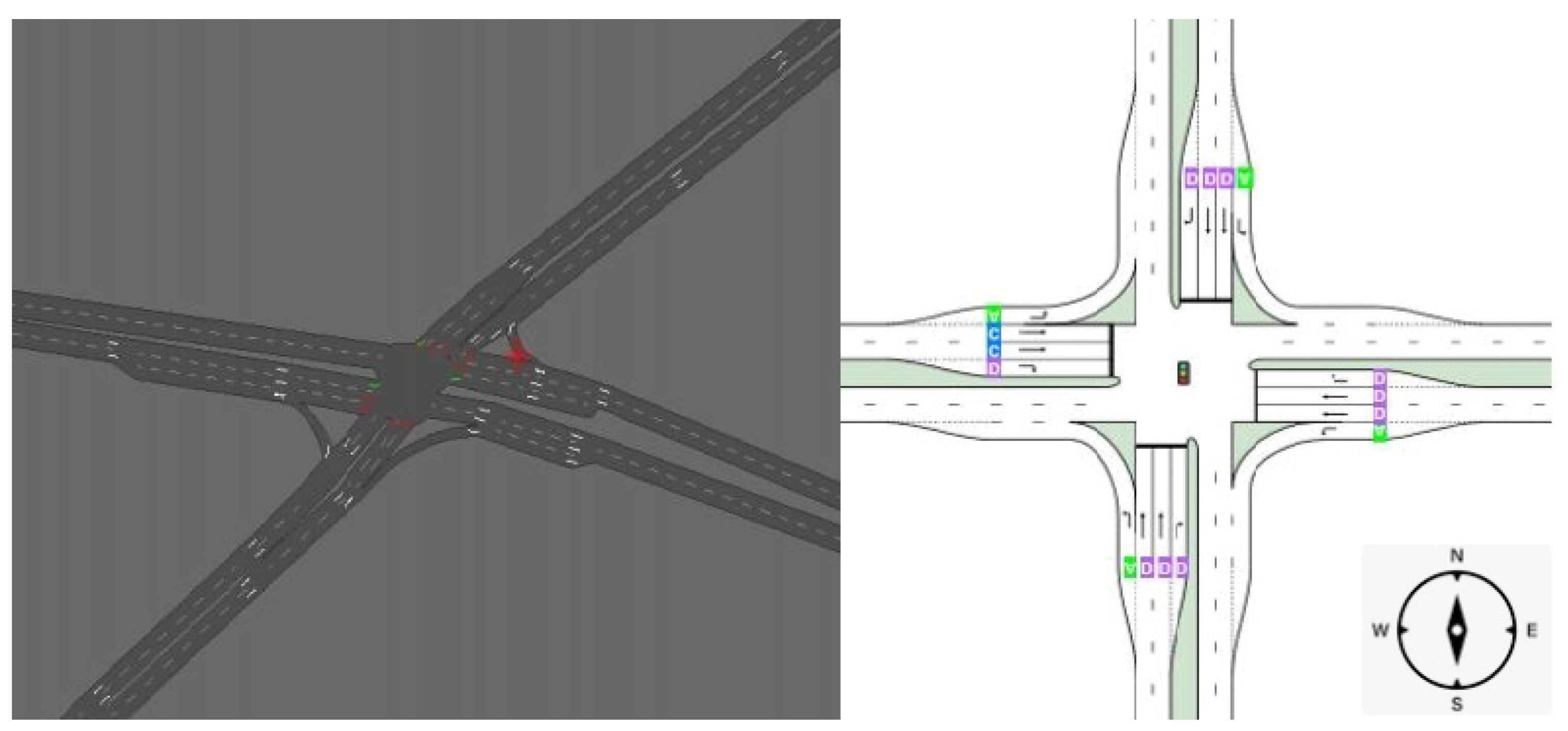
2.1. Dataset Description and Preparation
2.2. ARIMA Model
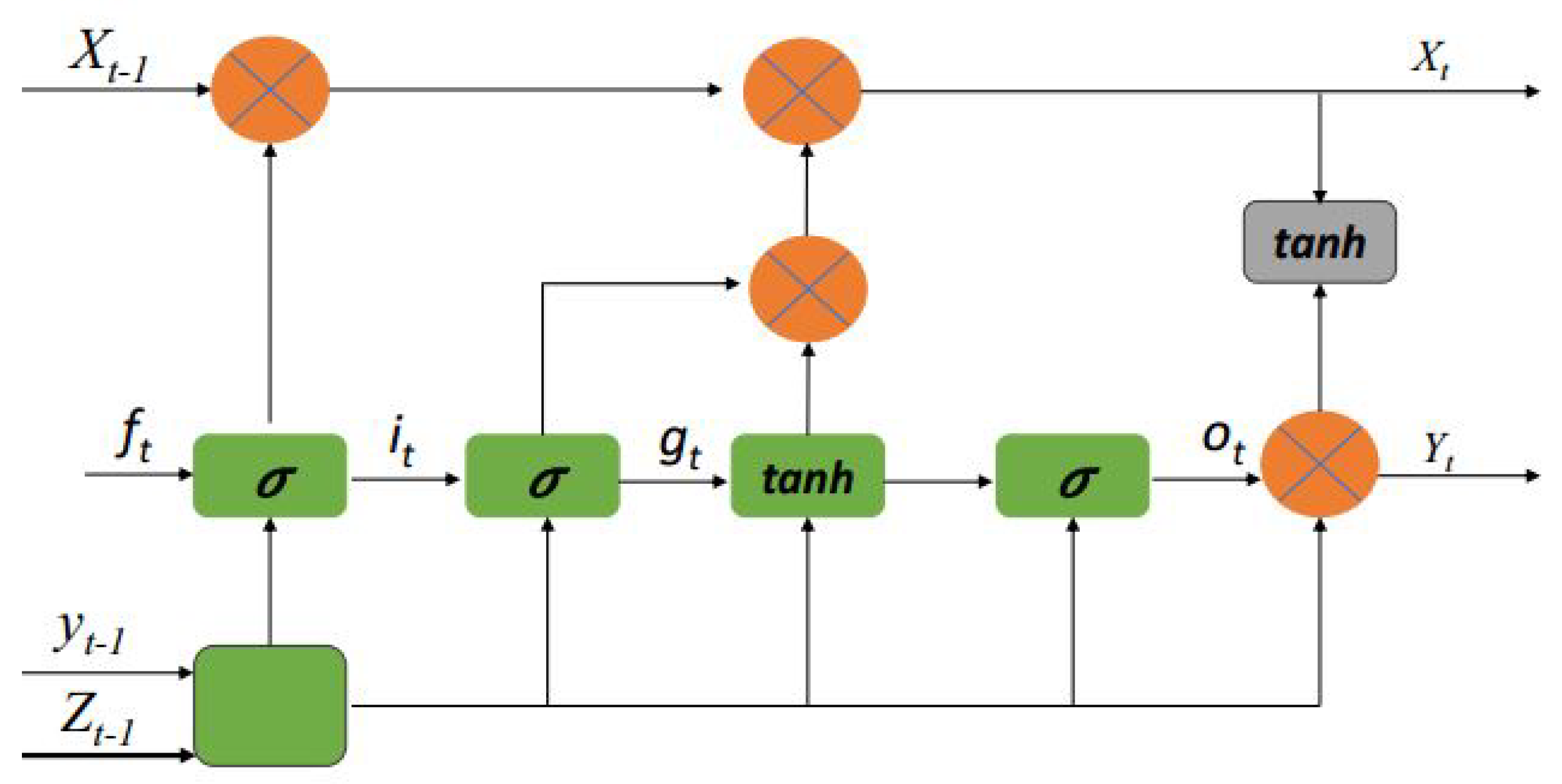
2.3. LSTM Model
2.4. Forecast Validation
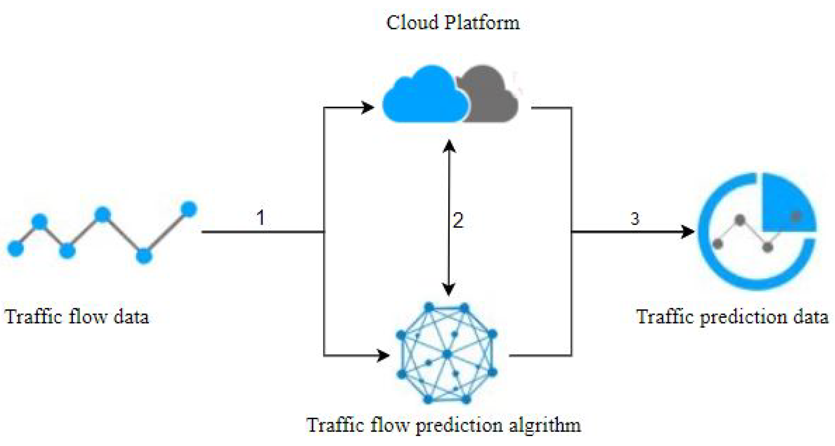
2.5. Design of Adaptive Traffic Flow Prediction Embedded System
3. Results and Discussion
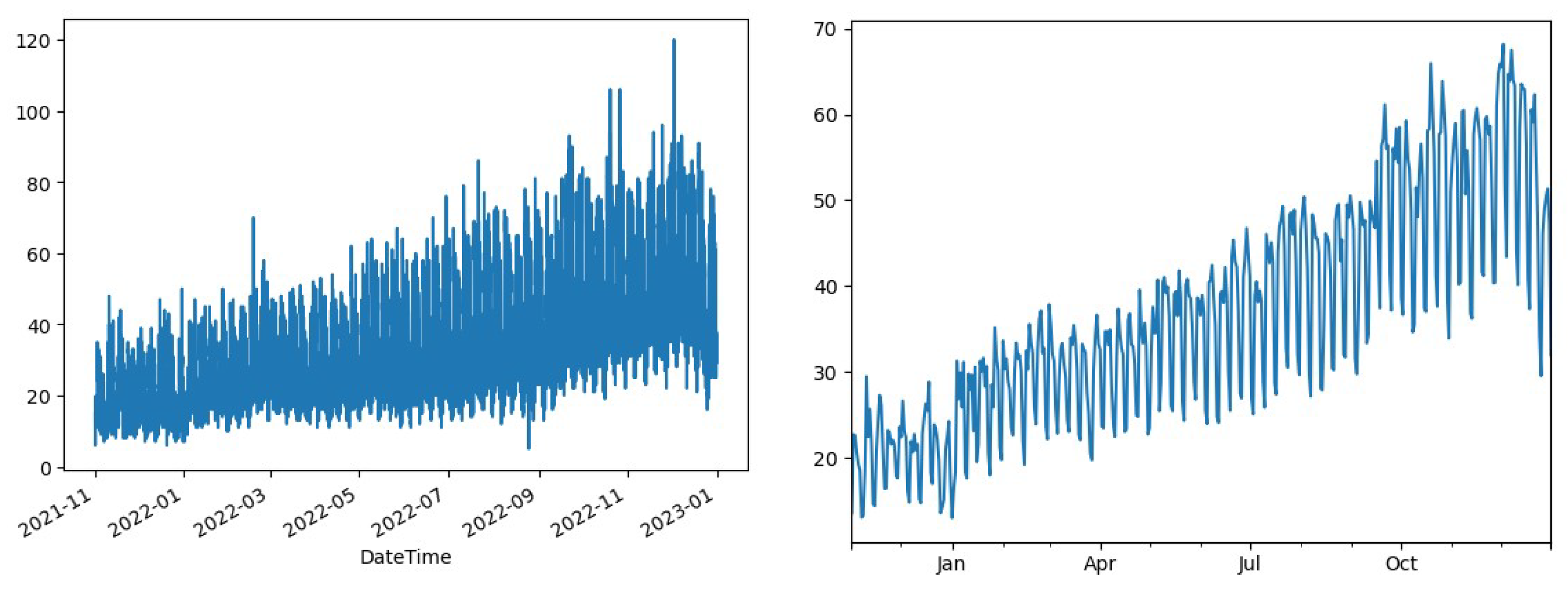
3.1. Traffic Trend at the Area
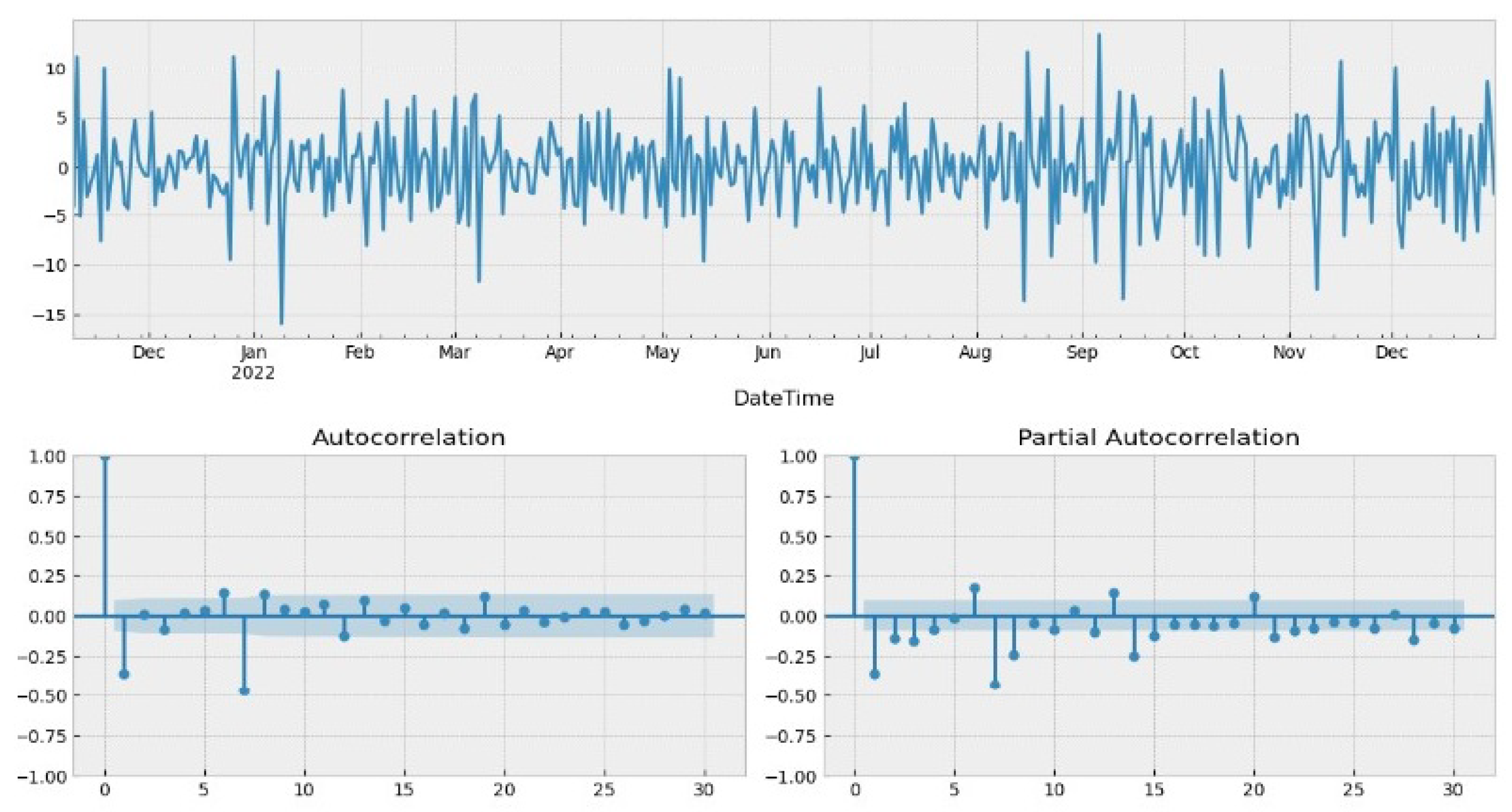
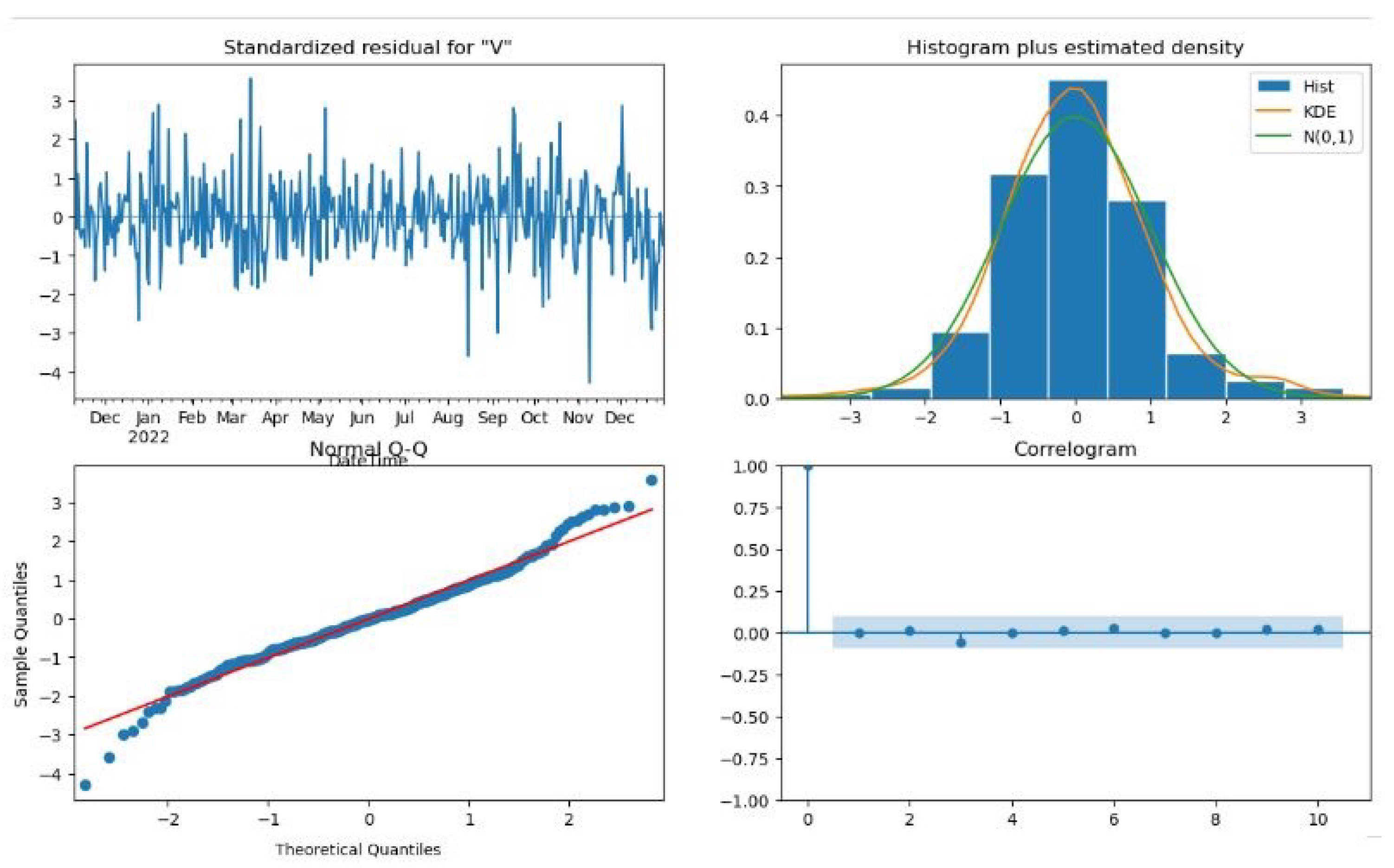
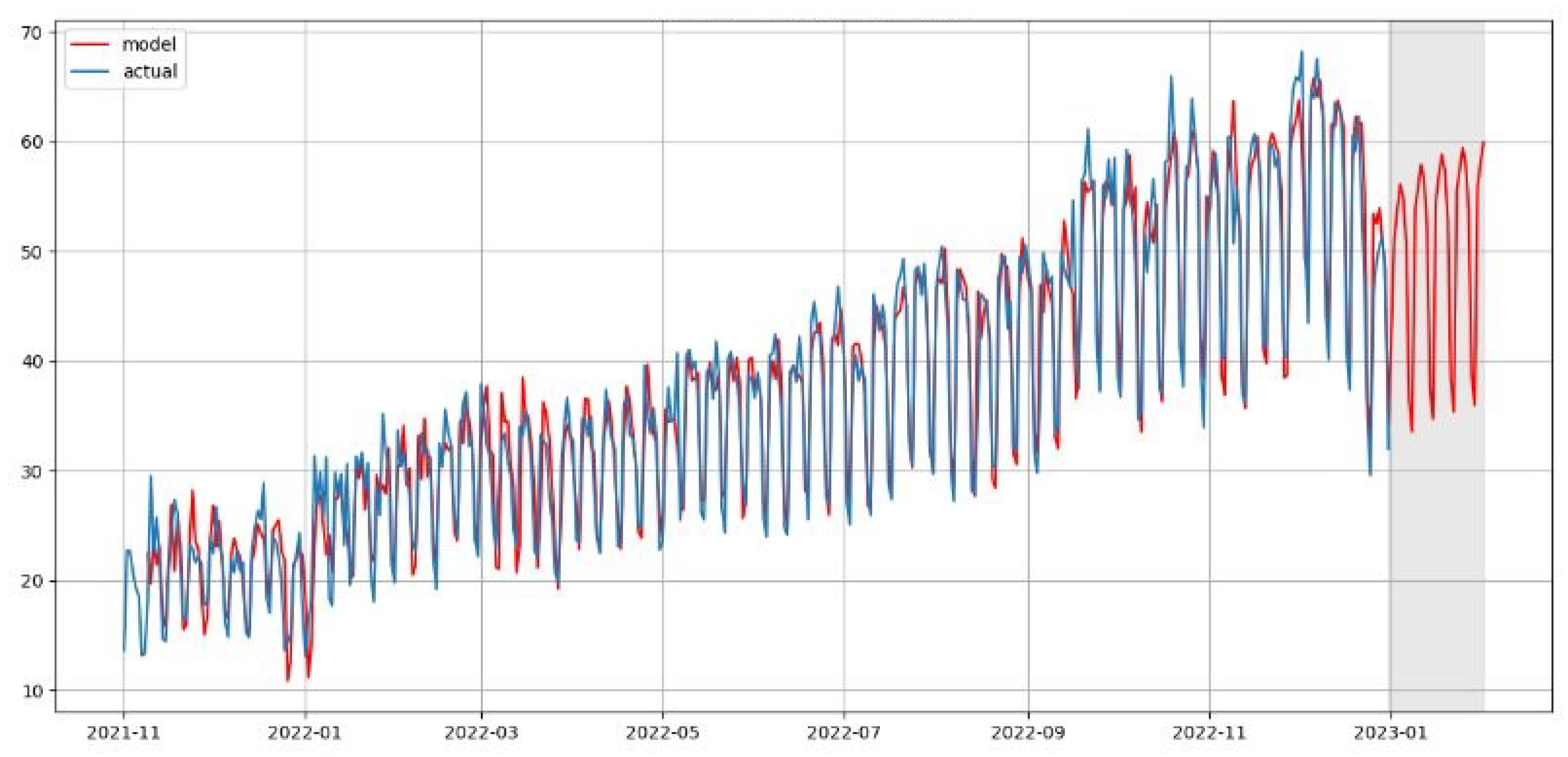
3.2. Fitting Models with ARIMA Model
3.3. Fitting Models with LSTM Model
3.4. Model Comparison
4. Conclusions
Author Contributions
Funding
Data Availability Statement
Conflicts of Interest
References
- Nasir, M.K.; Noor, R.; Kalam, M.A.; Masum, B.M. Reduction of fuel consumption and exhaust pollutant using intelligent transport systems. Sci. World J. 2014, 2014, 836375. [Google Scholar] [CrossRef] [PubMed]
- Gagliardi, G.; Lupia, M.; Cario, G.; Tedesco, F.; Cicchello Gaccio, F.; Lo Scudo, F.; Casavola, A. Advanced adaptive street lighting systems for smart cities. Smart Cities 2020, 3, 1495–1512. [Google Scholar] [CrossRef]
- Chen, C.; Liu, B.; Wan, S.; Qiao, P.; Pei, Q. An edge traffic flow detection scheme based on deep learning in an intelligent transportation system. IEEE Trans. Intell. Transp. Syst. 2020, 22, 1840–1852. [Google Scholar] [CrossRef]
- Florez, R.; Palomino-Quispe, F.; Coaquira-Castillo, R.J.; Herrera-Levano, J.C.; Paixão, T.; Alvarez, A.B. A CNN-Based Approach for Driver Drowsiness Detection by Real-Time Eye State Identification. Appl. Sci. 2023, 13, 7849. [Google Scholar] [CrossRef]
- Boukerche, A.; Wang, J. A performance modeling and analysis of a novel vehicular traffic flow prediction system using a hybrid machine learning-based model. Ad Hoc Netw. 2020, 106, 102224. [Google Scholar] [CrossRef]
- Meena, G.; Sharma, D.; Mahrishi, M. Traffic prediction for intelligent transportation system using machine learning. In Proceedings of the 2020 3rd International Conference on Emerging Technologies in Computer Engineering: Machine Learning and Internet of Things (ICETCE), Jaipur, India, 7–8 February 2020; pp. 145–148. [Google Scholar]
- Yuan, H.; Li, G. A survey of traffic prediction: From spatio-temporal data to intelligent transportation. Data Sci. Eng. 2021, 6, 63–85. [Google Scholar] [CrossRef]
- Lu, S.; Zhang, Q.; Chen, G.; Seng, D. A combined method for short-term traffic flow prediction based on recurrent neural network. Alex. Eng. J. 2021, 60, 87–94. [Google Scholar] [CrossRef]
- Chrobok, R. Theory and Application of Advanced Traffic Forecast Methods. Ph.D. Thesis, University of Duisburg-Essen, Duisburg, Germany, 2005. [Google Scholar]
- George, S.; Santra, A.K. Traffic prediction using multifaceted techniques: A survey. Wirel. Pers. Commun. 2020, 115, 1047–1106. [Google Scholar] [CrossRef]
- Zhao, Z.; Chen, W.; Wu, X.; Chen, P.C.; Liu, J. LSTM network: A deep learning approach for short-term traffic forecast. IET Intell. Transp. Syst. 2017, 11, 68–75. [Google Scholar] [CrossRef]
- Abduljabbar, R.L.; Dia, H.; Tsai, P.W.; Liyanage, S. Short-term traffic forecasting: An LSTM network for spatial-temporal speed prediction. Future Transp. 2021, 1, 21–37. [Google Scholar] [CrossRef]
- Alonso, B.; Musolino, G.; Rindone, C.; Vitetta, A. Estimation of a Fundamental Diagram with Heterogeneous Data Sources: Experimentation in the City of Santander. ISPRS Int. J. Geo-Inf. 2023, 12, 418. [Google Scholar] [CrossRef]
- Wu, T.; Chen, F.; Wan, Y. Graph attention LSTM network: A new model for traffic flow forecasting. In Proceedings of the 2018 5th International Conference on Information Science and Control Engineering (ICISCE), Zhengzhou, China, 20–22 July 2018; pp. 241–245. [Google Scholar]
- Wang, J.; Hu, F.; Li, L. Deep bi-directional long short-term memory model for short-term traffic flow prediction. In Proceedings of the Neural Information Processing: 24th International Conference, ICONIP 2017, Guangzhou, China, 14–18 November 2017; Proceedings, Part V 24. Springer: Berlin/Heidelberg, Germany, 2017; pp. 306–316. [Google Scholar]
- Kang, D.; Lv, Y.; Chen, Y.y. Short-term traffic flow prediction with LSTM recurrent neural network. In Proceedings of the 2017 IEEE 20th International Conference on Intelligent Transportation Systems (ITSC), Yokohama, Japan, 16–19 October 2017; pp. 1–6. [Google Scholar]
- Zhuang, W.; Cao, Y. Short-Term Traffic Flow Prediction Based on a K-Nearest Neighbor and Bidirectional Long Short-Term Memory Model. Appl. Sci. 2023, 13, 2681. [Google Scholar] [CrossRef]
- Tian, Y.; Zhang, K.; Li, J.; Lin, X.; Yang, B. LSTM-based traffic flow prediction with missing data. Neurocomputing 2018, 318, 297–305. [Google Scholar] [CrossRef]
- Yang, B.; Sun, S.; Li, J.; Lin, X.; Tian, Y. Traffic flow prediction using LSTM with feature enhancement. Neurocomputing 2019, 332, 320–327. [Google Scholar] [CrossRef]
- Lv, Y.; Duan, Y.; Kang, W.; Li, Z.; Wang, F.Y. Traffic flow prediction with big data: A deep learning approach. IEEE Trans. Intell. Transp. Syst. 2014, 16, 865–873. [Google Scholar] [CrossRef]
- Li, Y.; Chai, S.; Ma, Z.; Wang, G. A hybrid deep learning framework for long-term traffic flow prediction. IEEE Access 2021, 9, 11264–11271. [Google Scholar] [CrossRef]
- Wei, W.; Wu, H.; Ma, H. An autoencoder and LSTM-based traffic flow prediction method. Sensors 2019, 19, 2946. [Google Scholar] [CrossRef]
- Liu, B.; Cheng, J.; Liu, Q.; Tang, X. A long short-term traffic flow prediction method optimized by cluster computing. Electr. Electron. Eng. 2018, 1, 1–19. [Google Scholar]
- Navarro-Espinoza, A.; López-Bonilla, O.R.; García-Guerrero, E.E.; Tlelo-Cuautle, E.; López-Mancilla, D.; Hernández-Mejía, C.; Inzunza-González, E. Traffic flow prediction for smart traffic lights using machine learning algorithms. Technologies 2022, 10, 5. [Google Scholar] [CrossRef]
- Hafner, S.; Georganos, S.; Mugiraneza, T.; Ban, Y. Mapping Urban Population Growth from Sentinel-2 MSI and Census Data Using Deep Learning: A Case Study in Kigali, Rwanda. In Proceedings of the 2023 Joint Urban Remote Sensing Event (JURSE), Heraklion, Greece, 17–19 May 2023; pp. 1–4. [Google Scholar]
- Han, X.; Gong, S. LST-GCN: Long Short-Term Memory Embedded Graph Convolution Network for Traffic Flow Forecasting. Electronics 2022, 11, 2230. [Google Scholar] [CrossRef]
- Smith, B.L.; Williams, B.M.; Oswald, R.K. Comparison of parametric and nonparametric models for traffic flow forecasting. Transp. Res. Part C Emerg. Technol. 2002, 10, 303–321. [Google Scholar] [CrossRef]
- Shah, I.; Muhammad, I.; Ali, S.; Ahmed, S.; Almazah, M.M.; Al-Rezami, A. Forecasting day-ahead traffic flow using functional time series approach. Mathematics 2022, 10, 4279. [Google Scholar] [CrossRef]
- Nkurunziza, D.; Tafahomi, R. Assessment of Pedestrian Mobility on Road Networks in the City of Kigali. J. Public Policy Adm. 2023, 8, 1–20. [Google Scholar] [CrossRef]
- Lawe, S.; Wang, R. Optimization of traffic signals using deep learning neural networks. In Proceedings of the AI 2016: Advances in Artificial Intelligence: 29th Australasian Joint Conference, Hobart, TAS, Australia, 5–8 December 2016; pp. 403–415. [Google Scholar]
- Choi, B. ARMA Model Identification; Springer Science & Business Media: Berlin/Heidelberg, Germany, 2012. [Google Scholar]
- Xu, X.; Jin, X.; Xiao, D.; Ma, C.; Wong, S. A hybrid autoregressive fractionally integrated moving average and nonlinear autoregressive neural network model for short-term traffic flow prediction. J. Intell. Transp. Syst. 2023, 27, 1–18. [Google Scholar] [CrossRef]
- Awe, O.; Okeyinka, A.; Fatokun, J.O. An alternative algorithm for ARIMA model selection. In Proceedings of the 2020 International Conference in Mathematics, Computer Engineering and Computer Science (ICMCECS), Lagos, Nigeria, 18–21 March 2020; pp. 1–4. [Google Scholar]
- Williams, B.M.; Hoel, L.A. Modeling and forecasting vehicular traffic flow as a seasonal ARIMA process: Theoretical basis and empirical results. J. Transp. Eng. 2003, 129, 664–672. [Google Scholar] [CrossRef]
- Brockwell, P.J.; Davis, R.A. Introduction to Time Series and Forecasting; Springer: Berlin/Heidelberg, Germany, 2002. [Google Scholar]
- Hyndman, R.J.; Athanasopoulos, G. Forecasting: Principles and Practice; OTexts: Melbourne, Australia, 2018. [Google Scholar]
- Ishfaque, M.; Dai, Q.; Haq, N.u.; Jadoon, K.; Shahzad, S.M.; Janjuhah, H.T. Use of recurrent neural network with long short-term memory for seepage prediction at Tarbela Dam, KP, Pakistan. Energies 2022, 15, 3123. [Google Scholar] [CrossRef]
- Kontopoulou, V.I.; Panagopoulos, A.D.; Kakkos, I.; Matsopoulos, G.K. A Review of ARIMA vs. Machine Learning Approaches for Time Series Forecasting in Data Driven Networks. Future Internet 2023, 15, 255. [Google Scholar] [CrossRef]
- Kutlimuratov, A.; Khamzaev, J.; Kuchkorov, T.; Anwar, M.S.; Choi, A. Applying Enhanced Real-Time Monitoring and Counting Method for Effective Traffic Management in Tashkent. Sensors 2023, 23, 5007. [Google Scholar] [CrossRef]
- Sonnleitner, E.; Barth, O.; Palmanshofer, A.; Kurz, M. Traffic measurement and congestion detection based on real-time highway video data. Appl. Sci. 2020, 10, 6270. [Google Scholar] [CrossRef]
- Antoine, G.; Mikeka, C.; Bajpai, G.; Valko, A. Real-time traffic flow-based traffic signal scheduling: A queuing theory approach. World Rev. Intermodal Transp. Res. 2021, 10, 325–343. [Google Scholar] [CrossRef]
- Schizas, N.; Karras, A.; Karras, C.; Sioutas, S. TinyML for Ultra-Low Power AI and Large Scale IoT Deployments: A Systematic Review. Future Internet 2022, 14, 363. [Google Scholar] [CrossRef]
- Long, B.; Tan, F.; Newman, M. Forecasting the Monkeypox Outbreak Using ARIMA, Prophet, NeuralProphet, and LSTM Models in the United States. Forecasting 2023, 5, 127–137. [Google Scholar] [CrossRef]
- Sedai, A.; Dhakal, R.; Gautam, S.; Dhamala, A.; Bilbao, A.; Wang, Q.; Wigington, A.; Pol, S. Performance Analysis of Statistical, Machine Learning and Deep Learning Models in Long-Term Forecasting of Solar Power Production. Forecasting 2023, 5, 256–284. [Google Scholar] [CrossRef]


| Ref | Processing Technique | Predictive Performance Measure | Year |
|---|---|---|---|
| [5] | Forecasting method that is based on Graph Convolutional Network (GCN) and Attention-based sequence. | MAE, RMSE and R-Squared | 2020 |
| [8] | Forecasting method that is based on ARIMA model and LSTM neural network. | MAE, MSE, RMSE, and MAPE | 2021 |
| [11] | Short-term traffic forecast by using LSTM neural network. | MAE, MSE, RMSE, and mean relative error (MRE) | 2017 |
| [12] | Long Short-Term Memory (LSTM) recurrent neural network, Recurrent Neural Networks (RNNs), Modular Neural Networks (MNNs), Deep Learning Backpropagation (DLBP) and Radial Basis Function Networks (RBFNs). | MAPE and Accuracy (%) | 2021 |
| [17] | Forecasting method that is based on Bidirectional LSTM (BiLSTM), Support vector machines, GRU, KNN-LSTM, and CNN-LSTM models. | MAE, MSE, MAPE | 2023 |
| [21] | Forecasting method that is based on Graph convolutional network (GCN) and bi-directional LSTM (Bi-LSTM). | MAE, MAPE, and RMSE | 2022 |
| [26] | Long Short-Term Memory Graph convolutional network (LST-GCN) to road segments data. | MAE, MAPE, and RMSE | 2022 |
| [27] | ARIMA, Random Walk Forecast, and Deviation from historical average. | root mean square error of prediction (RMSEP), mean absolute deviation (MAD) and MAPE | 2002 |
| [28] | Forecasting day-ahead traffic flow using functional time series approach (FAR) and ARIMA. | MAE, MSE, MAPE, mean squared percentage error (MSPE) and mean absolute percentage error (DS-MAPE) | 2022 |
| Parameter | Value |
|---|---|
| Count | 30,452 |
| mean | 19.96 |
| std | 16.57 |
| min | 1 |
| 25% | 9 |
| 50% | 14 |
| 75% | 26 |
| Period of the Day | Pick Hour |
|---|---|
| AM Peak | 0800 h to 0900 h |
| PM Peak | 1700 h to 1900 h |
| Model | MAE | MAPE (%) | RMSE |
|---|---|---|---|
| LSTM | 10.282 | 22.519 | 5.852 |
| ARIMA | 10.884 | 24.232 | 9.138 |
Disclaimer/Publisher’s Note: The statements, opinions and data contained in all publications are solely those of the individual author(s) and contributor(s) and not of MDPI and/or the editor(s). MDPI and/or the editor(s) disclaim responsibility for any injury to people or property resulting from any ideas, methods, instructions or products referred to in the content. |
© 2023 by the authors. Licensee MDPI, Basel, Switzerland. This article is an open access article distributed under the terms and conditions of the Creative Commons Attribution (CC BY) license (https://creativecommons.org/licenses/by/4.0/).
Share and Cite
Katambire, V.N.; Musabe, R.; Uwitonze, A.; Mukanyiligira, D. Forecasting the Traffic Flow by Using ARIMA and LSTM Models: Case of Muhima Junction. Forecasting 2023, 5, 616-628. https://doi.org/10.3390/forecast5040034
Katambire VN, Musabe R, Uwitonze A, Mukanyiligira D. Forecasting the Traffic Flow by Using ARIMA and LSTM Models: Case of Muhima Junction. Forecasting. 2023; 5(4):616-628. https://doi.org/10.3390/forecast5040034
Chicago/Turabian StyleKatambire, Vienna N., Richard Musabe, Alfred Uwitonze, and Didacienne Mukanyiligira. 2023. "Forecasting the Traffic Flow by Using ARIMA and LSTM Models: Case of Muhima Junction" Forecasting 5, no. 4: 616-628. https://doi.org/10.3390/forecast5040034