An Extended Analysis of Temperature Prediction in Italy: From Sub-Seasonal to Seasonal Timescales

Abstract

Earth system predictions, from sub-seasonal to seasonal timescales, remain a challenging task, and the representation of predictability sources on seasonal timescales is a complex work. Nonetheless, advances in technology and science have been making continuous progress in seasonal forecasting. In a previous paper, a performance for temperature prediction by a modelling system named e-kmf^® was carried out in comparison with observations and climatology for a year of data; a low level of predictability in the sub-seasonal range, particularly in the second month, was observed over the Italian peninsula. Therefore, in this study, we focus our investigations specifically on the performance between the fifth and the eighth week of temperature forecasts over six years of simulations (2012–2018) to investigate the capability of the weather model to better reproduce the behavior of temperatures in the second month of the forecast. Although some differences in seasons are present, results have globally shown how temperature predictions have the potential to be quite skillful, with an average skill score of about 68%, with climatology used as reference; additionally, an overall anomaly correlation coefficient equal to 0.51 was shown, providing useful information for applications in planning, sales, and supply of natural energy resources.

1. Introduction and Context of Application

The use of weather forecasts is widely prevalent among governments, businesses, and individuals worldwide. The availability of accurate forecasts, ranging from a few hours to a few days in advance, significantly influences numerous decisions in various sectors of the global economy. As commercial activities, security concerns, and the management of natural resources become more intricate and globally interconnected due to climate change, the value and significance of weather and climate forecasts are expected to increase further [1,2]. While short-term forecasts already play a crucial role, many critical decisions may require advanced planning several weeks or even months ahead to anticipate favorable or disruptive environmental conditions [3]. The timely movement of emergency and disaster-relief supplies, which can take weeks or months, is a pertinent issue. Additionally, pre-positioning of resources in areas which are susceptible to an infectious disease outbreak, for instance, could save lives and optimize the effectiveness of limited resources.

There are numerous examples of instances where advanced planning and forecasting can be beneficial. For instance, naval and commercial shipping planners meticulously chart routes well in advance to strategically position assets, avoid potential hazards, and capitalize on favorable conditions [4]. By leveraging improved knowledge of precipitation and drought likelihood, farmers can make informed decisions when purchasing seed varieties, aiming to boost yields and minimize costs. Similarly, water resource managers face multiple decisions regarding reservoir levels over upcoming weeks, months, and seasons, considering water consumption and availability, particularly in regions where water scarcity necessitates wiser use of this vital resource [5].

Seasonal forecasts, which cover extended periods such as three months, provide insights into average oceanic and atmospheric conditions. These forecasts are typically issued with lead times ranging from a month to several seasons [6,7]. On the other hand, sub-seasonal forecasts extend over a week or more, with lead times typically ranging from 2 to 6 weeks [8]. While there have been improvements in seasonal and sub-seasonal predictions in recent years, there remains ample room for further enhancement in terms of accuracy, range of forecasted variables, and availability of regular forecast products [9,10]. The advancements in environmental prediction have immense potential to maximize various benefits, such as saving lives, protecting property, promoting economic growth, preserving the environment, and enabling well-informed policy decisions.

Despite this significant potential, predicting Earth system behavior on sub-seasonal–seasonal timescales remains a daunting task. While it is increasingly acknowledged that Earth systems exhibit multiple sources of predictability over seasonal timescales, effectively representing these sources is a complex undertaking. Models must accurately capture the initial conditions of the atmosphere, ocean, land surface, and cryosphere, as well as the interactions or coupling between these different components. Moreover, the longer lead times associated with seasonal predictions pose challenges in representing uncertainty and conducting verification, making it more computationally demanding than everyday numerical weather prediction. Nevertheless, advancements in technology and scientific understanding contribute to continuous progress in seasonal forecasting.

Another key challenge lies in enhancing the practical applicability of sub-seasonal–seasonal forecasts for users. These forecasts exhibit lower skill compared to shorter-term predictions and may involve communicating probabilistic information that is less familiar to many users [11,12]. Hence, following the needs of application in management of natural resource supply, a sub-seasonal–seasonal forecast was developed by the Eni company at the beginning of the previous decade, intended for applications in energy management [13]. In fact, the efficient organization of energy and gas distribution systems often requires outlook prediction which accounts for energy and gas demand, which is strictly related to weather and climatic trends [14,15,16]

For instance, Liu et al. [17] conducted a review that explores the historical trends and future challenges of natural gas consumption. They found that long-term forecasting is primarily influenced by variables in production, population, and economy. Medium-term forecasting, on the other hand, is mainly influenced by economic and temperature variables. In terms of short-term forecasting, temperature variables, weather conditions, and the type of date play a significant role as influencing factors. Therefore, a prevailing consideration is that sub-seasonal temperature forecasts in the two–twelve-week horizon between medium-range and seasonal–multi-seasonal prediction poses complex issues. Indeed, characterizing a sub-seasonal atmospheric forecast challenge is not as straightforward as a typical initial value weather forecast problem, where the time spans are shorter and there is a risk of losing initial value data, or a boundary value climate-prediction problem that relies on prescribed surface temperature anomalies to drive early seasonal climate forecast systems. Nonetheless, recent studies indicate the potential for predictability across all timescales, as highlighted by Hoskins [18] and the World Meteorological Organization [19]. Evidence suggests that a forecast model encompassing the ocean–atmosphere–ice–land system (as depicted in Figure 1) integrates information from initial conditions across the interconnected system, including slowly changing components, such as the ocean, sea ice, and land hydrology. Consequently, this integrated model yields sub-seasonal forecasts that demonstrate considerable skill in traditional weather variables, often comparable to seasonal forecasts, as observed in research conducted by Dutton et al. [20,21].

Moreover, in the sub-seasonal range, different techniques have been used to improve temperature forecasts, including machine learning [22,23], statistical models trained on dynamical models [24], and data-driven methods using random forest techniques [25].

Under this framework, in this current study, we extended a past investigation [13] where a benchmark analysis was only shown on data of one year for sub-seasonal and seasonal forecasts of temperatures by our meteorological model. The application of the model was intended to support the prediction of energy demand and improve the management, purchase, and sale of natural gas stocks [26]. The analysis primarily focused on assessing the long-term temperature predictions of two models, specifically the eni-kassandra meteo forecast (e-kmf^®) and CFS-NCEP (Climate Forecast System—National Centers for Environmental Prediction), across three regions in Italy (north, center, and south, excluding the main Italian islands). In order to evaluate these models, daily temperature forecasts were collected from regular initialization runs. These forecasts were then averaged to create weekly predictions for each model grid point within the three macro areas of Italy. Subsequently, the temperature forecasts were further averaged to derive a single temperature prediction for each week in each macro area. By employing the mean absolute error (MAE) metric, it was observed that the e-kmf^® model outperformed the CFS-NCEP model in the majority of areas and forecast-initiation months. On average, the e-kmf^® model demonstrated a skill at 35% compared to climatology, which signifies a statistical analysis of weather conditions observed from 1984 to 2008 used as a reference for the data of the specific year being analyzed. During the initial month of the forecast, the e-kmf^® model exhibited a strong correlation between the predicted and measured temperature data. However, a decline in model performance was noticed between the 5th and 8th week of the prediction period.

Therefore, this paper specifically addresses this last critical issue: analyzing temperature forecasts against observations and climatology in this sub-seasonal range over several years of forecast (2012–2018) for the same three macro areas of Italy, with the same adopted methodology. In particular, the behavior of our model in the sub-seasonal range has been analyzed here, considering that some anomalies appeared for the 2010 simulations in the previous study; hence, this study explored the question of whether those variances depend on some peculiarities of that particular year (2010), instead of some model biases which turned out to be mostly depending on inner sources of predictability of that year, and not by a general model’s bias. Since the model has been developed, we have now analyzed this sub-seasonal range forecasts, keeping the model version and the climatological mean unchanged, without modifying the reference data. Hence, the aim of this study is to quantify, through statistical indexes, how temperature forecasts from the meteorological model perform in respect to the observed data and climatological behavior for the three Italian macro areas in the sub-seasonal range, particularly in the second month of the forecast.

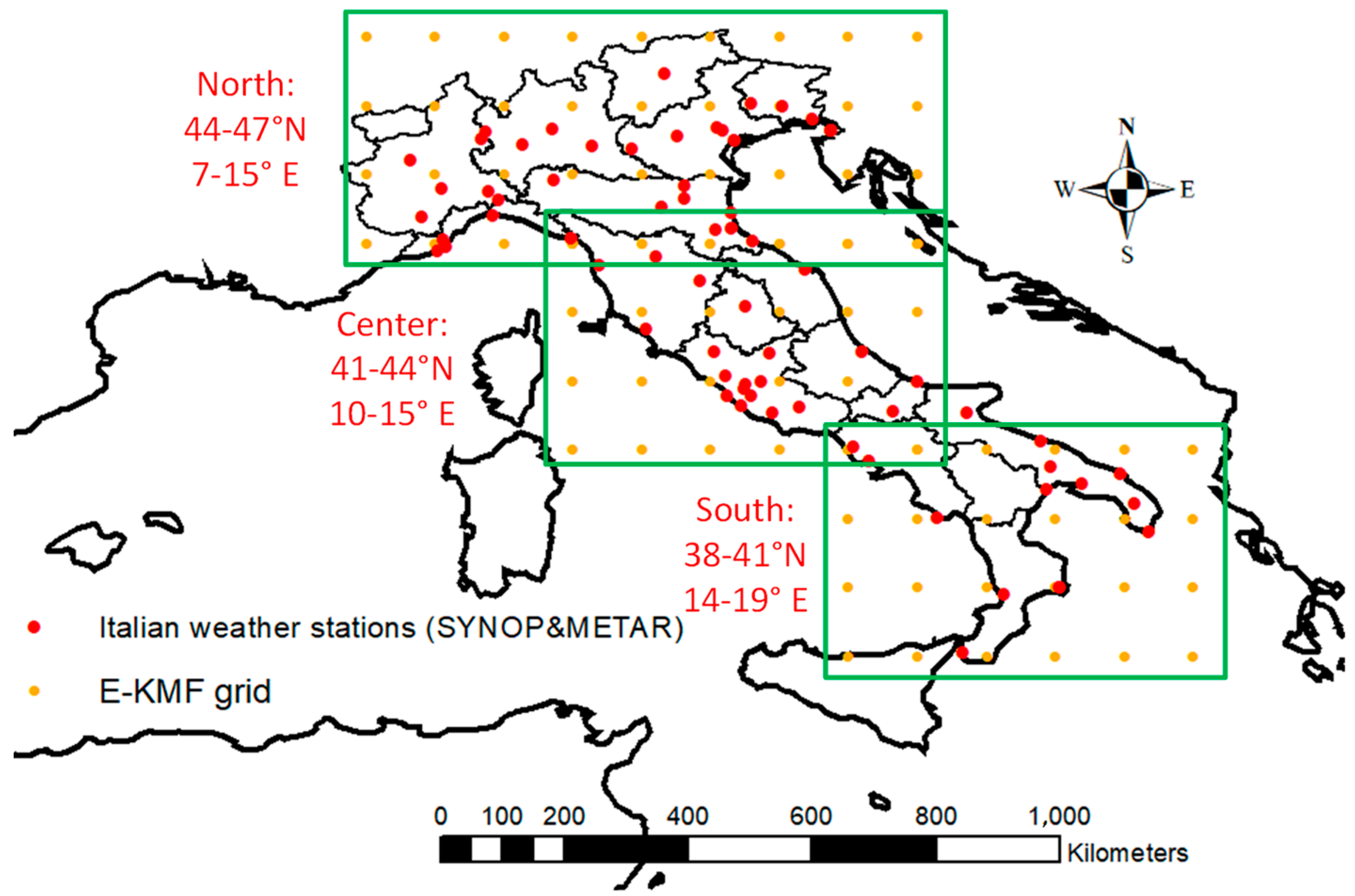
2. The Area of Study

The focus of this study is the Italian peninsula, which has been divided into three sub-regions or macro areas: north, center, and south (as shown in Figure 2). These divisions are based on the major climate variations across the country, as well as the differences in energy demand and market. The Po Valley, located in the northern region, stands out as the most densely populated and industrialized area, with a high energy consumption rate. In contrast, central and southern Italy have lower population densities and exhibit comparatively lower energy demands. The climate in northern Italy is predominantly characterized by a humid continental climate, primarily influenced by the presence of the Po Valley. On the other hand, central and southern Italy, along with the coastal areas in the northern regions, experience a Mediterranean climate. Additionally, the Italian climate is significantly influenced by two prominent mountain ranges, namely the Alps and the Apennines. These mountains play a crucial role in shaping the weather patterns across the country. Situated in the middle of the Mediterranean basin, the Italian Peninsula is subject to various factors that impact its weather and climate. The passage of cyclonic systems and associated fronts largely controls the weather conditions, and their occurrence and frequency are influenced by the distribution of land masses, sea surface temperature gradients, and the orientation of baroclinic zones. The Mediterranean area is highly populated by cyclones, especially in the winter season, determining the weather and climate [27], despite being located south of the global mid-latitude climatic belt. The Mediterranean region possesses a complex geography characterized by various landforms, such as mountains, basins, gulfs, islands, and peninsulas. The Mediterranean Sea is encircled by towering mountain ranges on almost all sides, resulting in distinct climatic patterns compared to other parts of the world. Among these mountain ranges, the highest is the Alps, which soar up to 4800 m and experience extensive snowfall during winter. The presence of islands, peninsulas, regional seas, and basins further adds to the intricate distribution of land and sea in the region. These geographical features have significant implications for both the circulation of sea and atmosphere, creating substantial spatial variations. Additionally, the abundance of sub-regional land mesoscale features complicates short- and medium-term predictions.

Nonetheless, planetary-scale patterns exert a significant influence on the climate of the Mediterranean region. The intricate nature of regional characteristics, which are influenced by these large-scale forces, adds complexity in terms of temporal and spatial behavior. The interplay between orography, the physical features of the land, and the distribution of land and sea is crucial in shaping the climate on a basin level and establishing its connections with global weather patterns. The intricate nature of basin topography gives rise to mesoscale features and inter-seasonal variations, which would otherwise be more uniform and enduring. Most studies [28,29,30] considered winter and summer regimes especially, while characterizations of spring and autumn are more uncertain; this reveals, presumably, the transient nature of these two seasons in the Mediterranean region.

3. Model and Data Analysis

This section provides a description of the model and measurements used in this study, focusing on temperature data for both climatology and daily observations. The statistical analysis procedure is also outlined, which closely follows the approach developed by [13]. The evaluation of temperature forecasts includes commonly used standard statistical indexes found in scientific literature [31,32,33]. These metrics are utilized to assess the reliability of 2 m air temperature forecasts in three specific geographical areas in Italy, namely the north, center, and south. The statistical analysis involves comparing the model forecasts and the climatological mean with the observed temperature data for the second month. Specifically, the second month refers to an average of the 5th, 6th, 7th, and 8th weeks. The analysis covers the years between 2012 and 2018, with a focus on the lead time forecast.

3.1. The Kassandra Meteo Forecast Model

The e-kmf^® global forecast system employs a combination of models and ensemble techniques [34,35,36,37] to generate temperature predictions for different timeframes. These forecasts encompass short–medium terms, typically ranging from 1 to 10 days, as well as sub-seasonal periods of approximately 2–12 weeks [38]. Short- and medium-term predictions utilize regional and limited area models (LAMs), with grid sizes varying from 1.25 km to 10 km. On the other hand, long-term forecasts, such as the one in this case study, involve two global models with 20 perturbed initial conditions, along with one control member, resulting in a multi-model ensemble of 40 forecasts plus two control members. While the e-kmf^® system currently utilizes global models with improved horizontal and vertical resolution, historical data from 2012 to 2018 were obtained using the same models as described in [13]. The first global model employed had a horizontal spectral triangular truncation of 126 waves (T126) and 42 sigma pressure hybrid layers (L42). The second model was a modified global version of the WRF-ARW (Weather Research and Forecasting—Advanced Research WRF) model, featuring 42 vertical levels and a horizontal grid of approximately 90 km. The resulting output of the multi-model ensemble is presented on a regular latitude–longitude grid with a spacing of 1°, providing temporal outputs every 6 h and a forecast horizon of 90 days. Initial conditions are derived from the global forecasting system (GFS) model’s initial condition, which is based on the grid-point statistical interpolation (GSI) global data assimilation system (GDAS) and incorporates a 3D-Var method to continuously update the background fields used for the initial condition. The model incorporates global sea surface temperature (SST) boundary conditions [39], utilizing SST anomaly simulations from a mixed-layer model. Each ensemble simulation employs various physical and dynamical schemes for micro-physics [40,41], the planetary boundary layer (PBL), the surface layer [42,43,44,45,46,47], cumulus parameterization [48,49], radiation [50,51,52], and land surface physics [53,54,55,56]. In the proposed benchmark, a selection process is applied to the ensembles of the two models to obtain a single value which can be compared with observed and climatological data. This procedure involves computing a measure based on the distance between each member and the best member of the ensembles. Various normalized model variables are used for this computation, and values outside of a predefined range are excluded based on this measure. The overall final value is obtained by taking a weighted average of the remaining members, which are also used to provide boundary conditions to the local ensemble prediction system (LEPS) for high-resolution forecasts in limited areas.

3.2. Observations and Climatology

The weather stations used in the previous analysis, both for climatology and daily observations, are maintained with the same characteristics as those employed in the present study. Data from various official weather stations located in the three macro areas in Italy were utilized, as documented in ([13],

Table 1. The MAE for all years over the three Italian areas.

North			Center			South
	Clima	e-kmf®		Clima	e-kmf®		Clima	e-kmf®
2012	1.68	0.85		1.78	0.91		1.39	0.60
2013	1.18	0.77		1.19	0.83		0.98	0.54
2014	1.81	1.03		1.67	1.00		1.21	0.77
2015	1.45	0.76		1.37	0.65		0.94	0.46
2016	1.05	0.57		1.15	0.65		0.76	0.44
2017	1.60	0.70		1.56	0.71		1.00	0.51
2018	1.62	0.84		1.71	0.63		0.94	0.30

). The observations were conducted between 2012 and mid-2018, utilizing the SYNOP (surface synoptic observations) and METAR (meteorological aerodrome report). Temperature readings were recorded at intervals ranging from half-hourly to three-hourly each day and stored in a database to compile comprehensive observational information. To facilitate a long-term comparison between forecasts and observations, temperature data were aggregated to generate weekly mean values for each reference area in Italy (north, center, and south). These weekly mean values were then utilized for both comparing observed and forecasted data and constructing the climatology for each reference area. The same 25-year reference period (1984–2008) used in the previous study was equally kept for a homogeneity of comparison. Lastly, a mean climatological temperature value for the second month ahead has been obtained and used as reference for the current comparison with observations and forecasts.

3.3. Methodology of the Benchmark Analysis

The 2 m temperature forecasts by e-kmf^® model were evaluated by comparing them to observed data and climatology. This evaluation involved the use of straightforward statistical indexes to assess the model performance. The analysis focused on the weekly forecasted data for three macro areas, employing the same methodology as proposed by [13]. This means that each macro area’s weekly forecast was obtained according to the following Equations (1)–(4):

$${\overline{T}}^i{}_{j,k,d}=\frac{1}{4}{\displaystyle \sum _{i=1}^4{T}_{j,i,d,k}}$$

(1)

$${\overline{{\overline{T}}^i}}^k{}_{j,d}=\frac{1}{5}{\displaystyle \sum _{k=1}^5{\overline{T}}^i{}_{d,j,k}}$$

(2)

$$T{w}_j=\frac{1}{7}{\displaystyle \sum _{d=1}^7{\overline{{\overline{T}}^i}}^k{}_{j,d}}$$

(3)

$$Ta=\frac{1}{N}{\displaystyle \sum _{j=1}^{N}T{w}_j}$$

(4)

where $T_{j,i,d,k}$ is the air temperature in the grid point, j, for the six-hour time interval, i, of the simulated day, d, corresponding to the model initialization, k; ${\overline{T}}^i{}_{j,k,d}$ is the mean daily temperature of the day, d, in the grid point, j, corresponding to the model initialization, k; ${\overline{{\overline{T}}^i}}^k{}_{j,d}$ is the mean daily temperature of the day, d, in the grid point, j, averaged over the model initializations; $T{w}_j$ is the mean weekly temperature in the grid point, j; $T{a}_j$ is the mean weekly temperature averaged over the N grid points within the macro area.

Since the aim of the study was to determine the performance of the model for the second month ahead, once the weekly means were obtained, the temperature forecasts of the 5th, 6th, 7th, and 8th weeks were averaged out to obtain one single value to be compared with climatology and observed data.

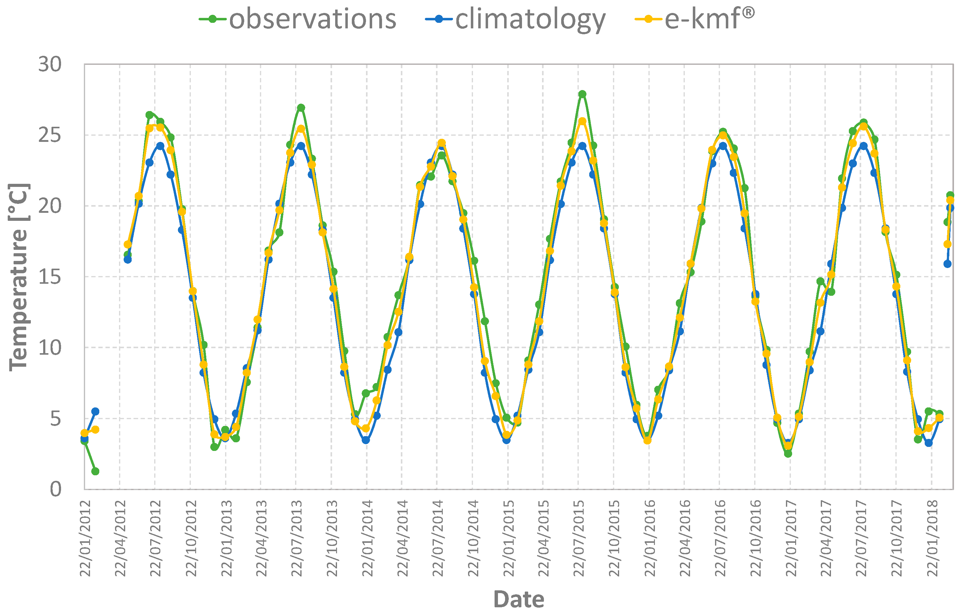
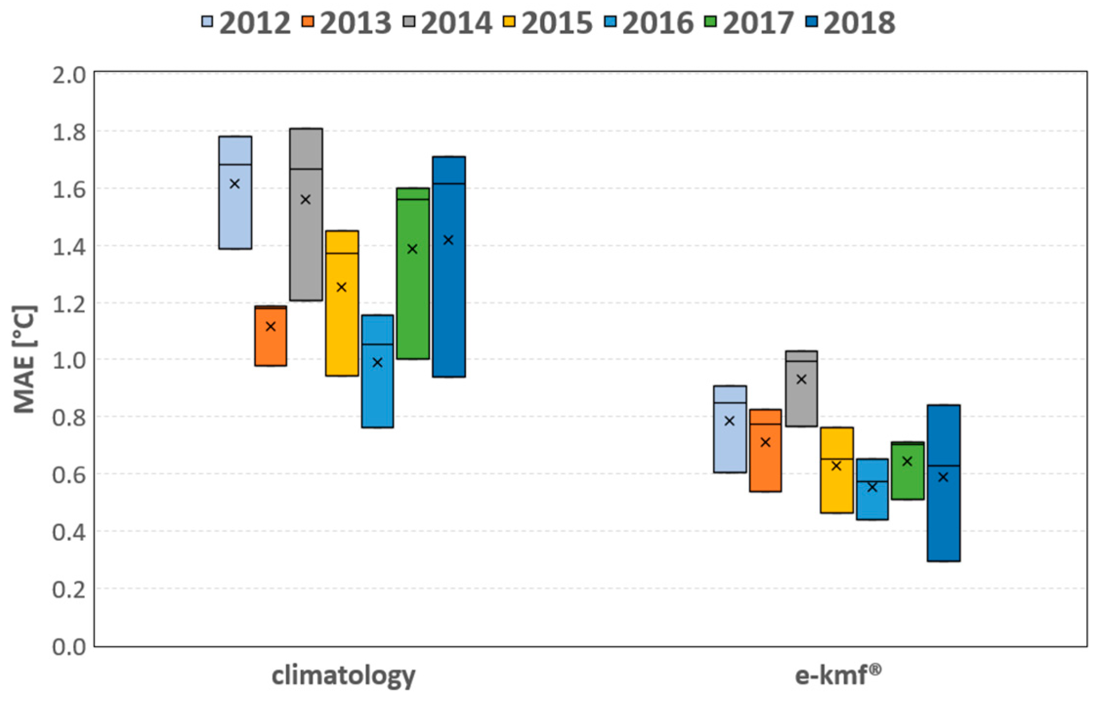
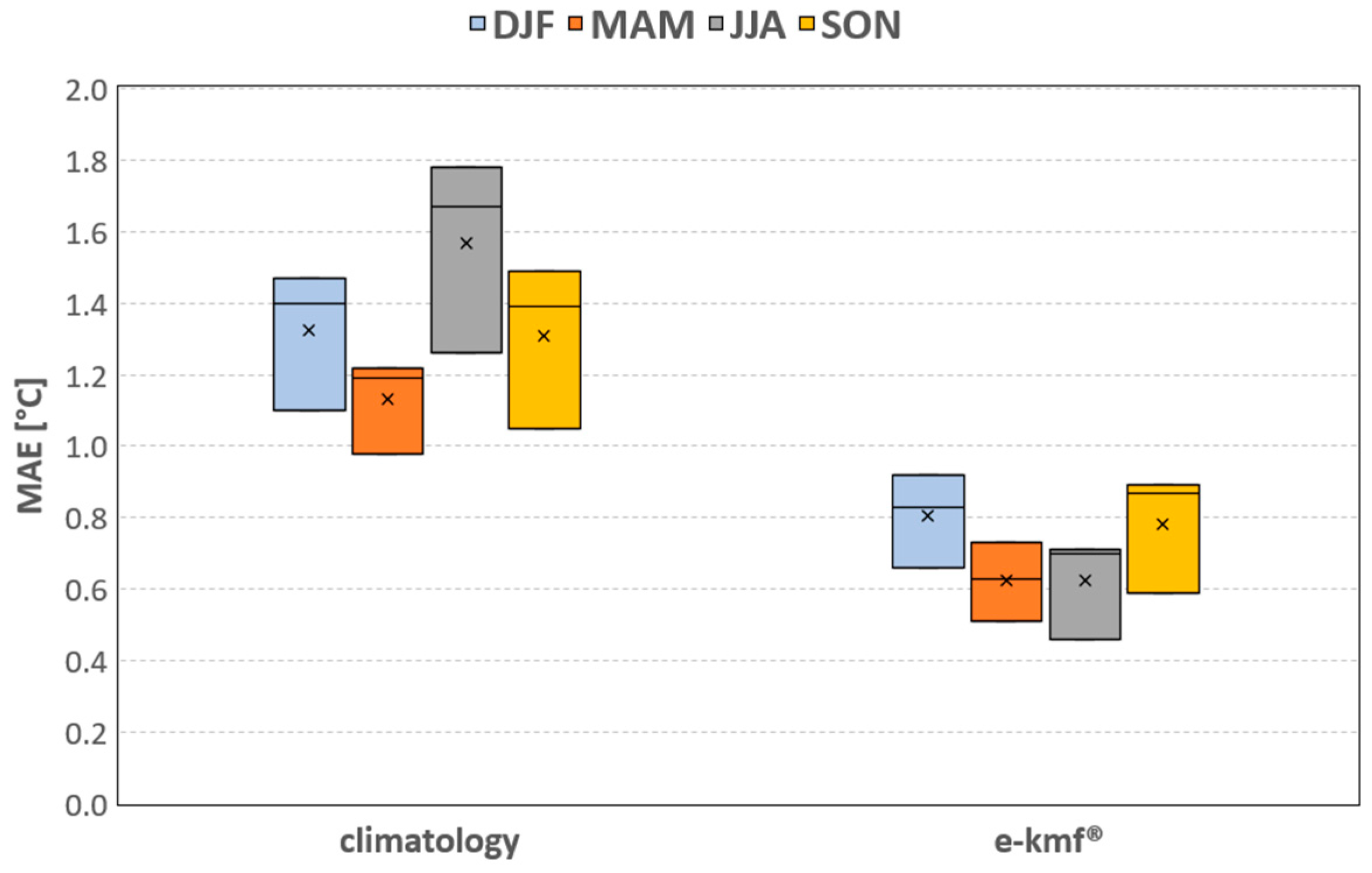
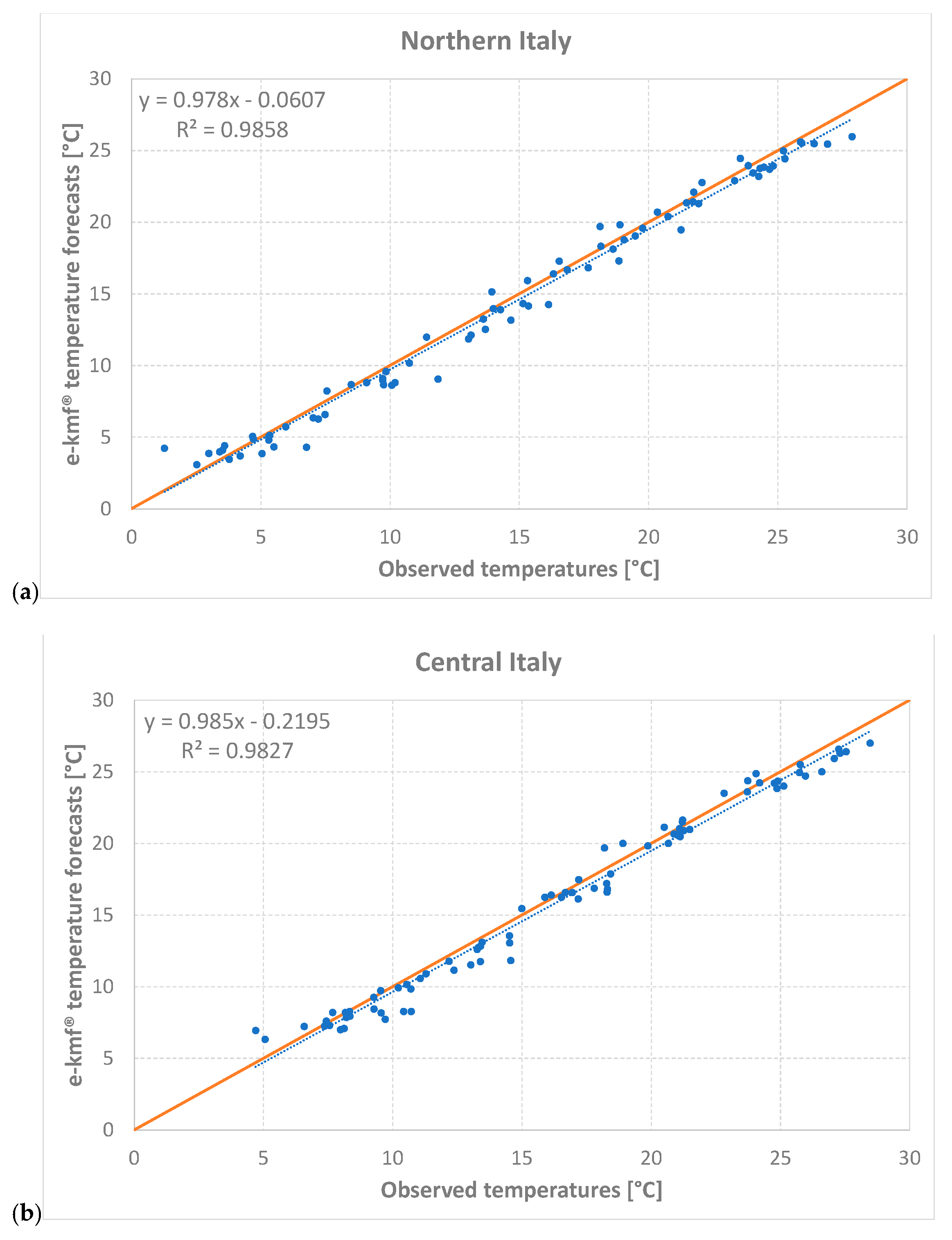
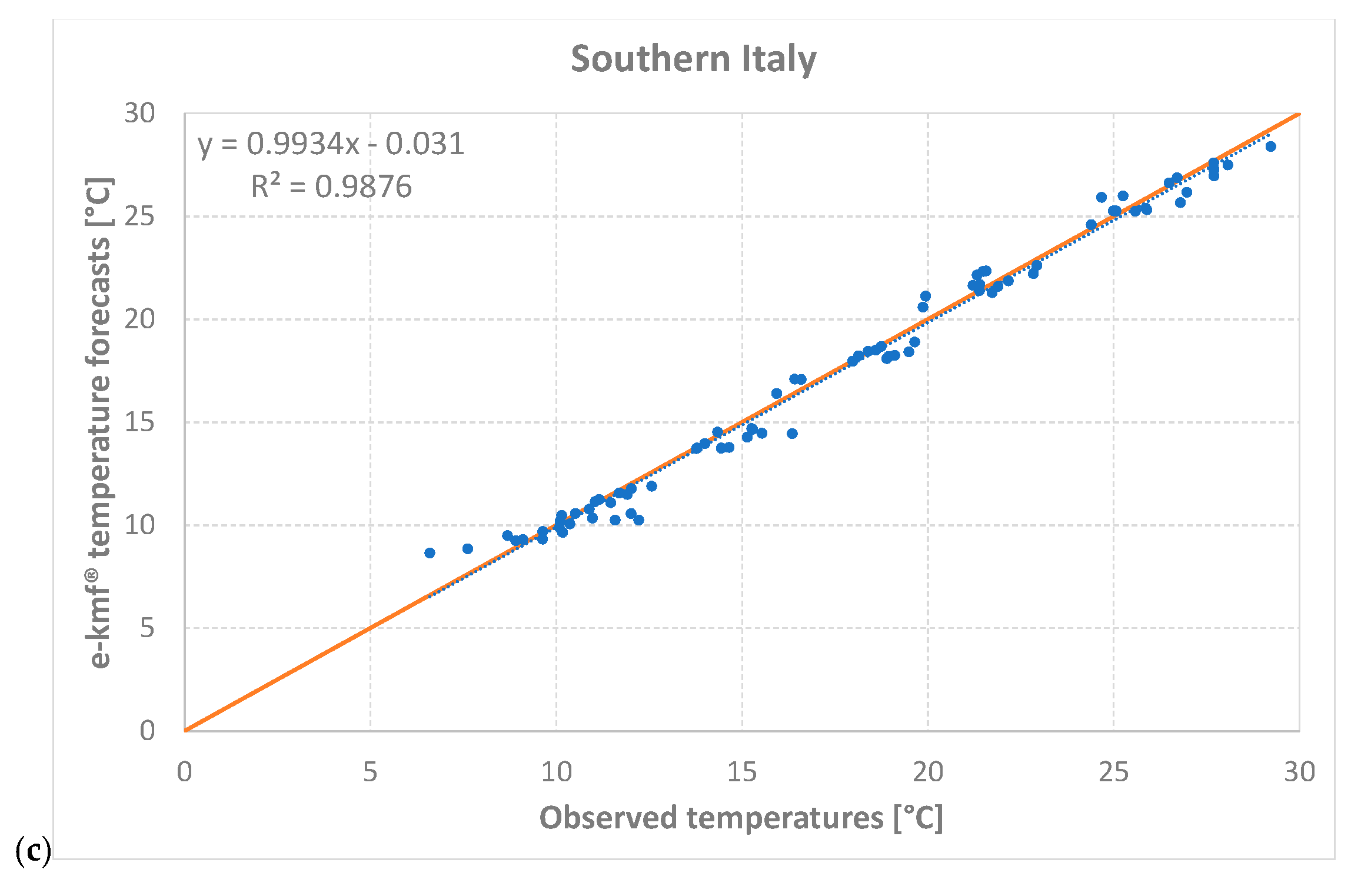
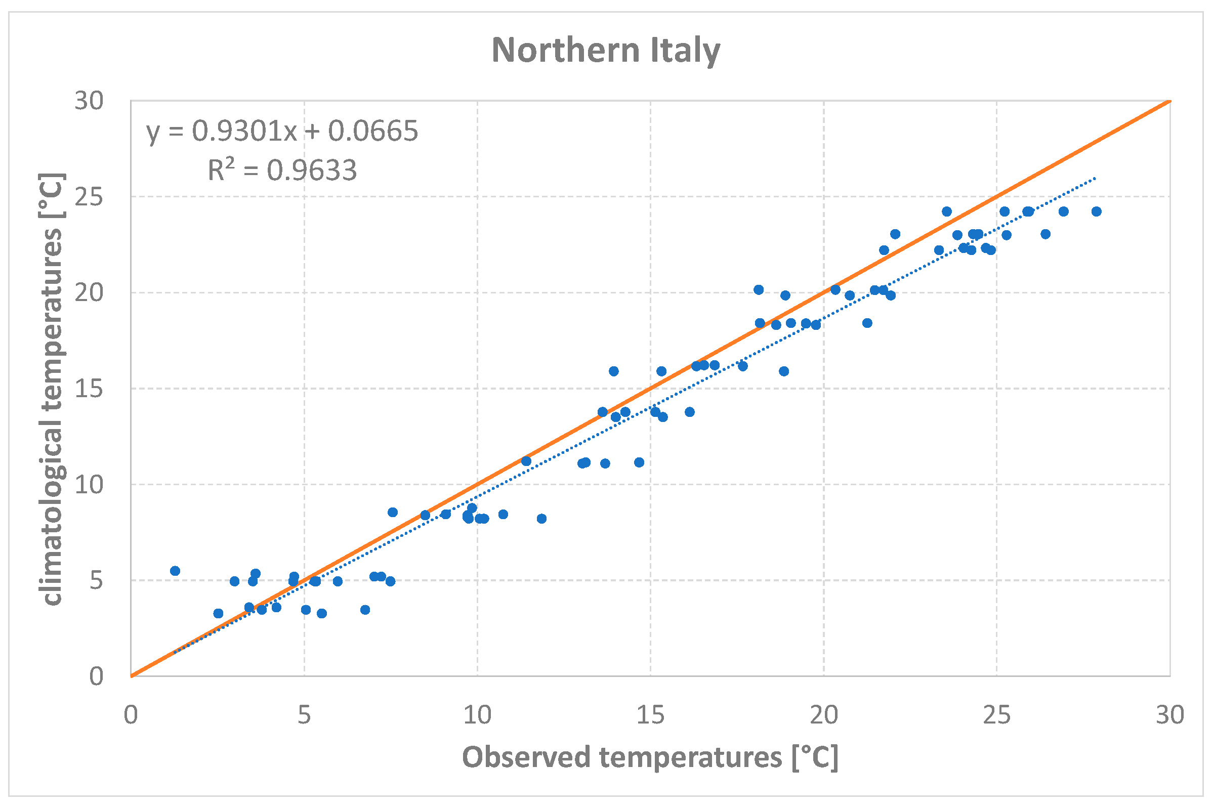
4. Results and Discussion

In order to assess the predictability and reliability of the temperature forecasts and to analyze their performance, a statistical analysis was conducted. This analysis involved comparing the forecast model and climatology mean during the observation period (2012–2018). The results presented here focus on the performance of the second month as a lead time forecasted by our e-kmf^® model; no further comparisons with other existing forecast systems were carried out in the current study. The evaluation employed three indexes: the mean absolute error (MAE), the climatological skill score (SS_clim), and the anomaly correlation coefficient (ACC). These indexes were used to evaluate and discuss the performance of the temperature forecasts.

Data Analysis

A graphical sequence during the observation period (OP) is shown in Figure 3 for the observed, climatological, and e-kmf^® model data for the second month of the forecast for the northern Italy macro area. Comparable picture sequences have been obtained for central and southern Italy (not shown here for the sake of brevity).

At first sight, a good match by the e-kmf^® model with observed data is shown, although a general underestimation is present over the six analyzed years, especially for historical climatological data. This is especially evident when looking at Figure 4, where the MAE for each year of the OP is illustrated, and a difference of about 1 °C among the two sets of data is displayed. This slight underestimation of the 2 m temperature for each year in all areas is much greater for the climatological data than for the e-kmf^® forecast: in fact, a mean bias is found to be 0.94 and 0.98 in the analyzed OP, respectively. This is an expected result, since all these years have been generally warmer than normal throughout Italy ([57], periodically updated here: www.isac.cnr.it/climstor, accessed on 27 September 2023).

Table 1 summarizes the MAE for each year in the OP for the climatological and e-kmf^® forecast data over the three macro areas. The mean absolute error for the three macro areas is calculated as follows (Equation (5)):

$$\mathrm{M}\mathrm{A}\mathrm{E}=\frac{1}{n}{\sum }_{i=1}^n|F_i-O_i|$$

(5)

where O_i is the observed value, F_i is the forecasted or climatological value, and n is the number of analyzed data.

These achieved outcomes are independent from areas or seasons, as shown in Figure 5, where the model indicates a better performance in summer and a lower performance in winter, in agreement with the Mediterranean climate of the area [58]. As expected, the MAE for the climatological data (with an overall underestimation of temperatures) is nearly the same for winter and autumn, and slightly lower in summer.

Compared to the previous analysis of data from 2010 [13], in this paper, better results have been obtained by the e-kmf^® model in the sub-seasonal prediction range. In fact, overall values of MAE were equal to 1.74 °C, 1.29 °C, and 1.20 °C for the second month of forecast in the north, center, and south of Italy, respectively; meanwhile, in the current study, we achieved scores below 1 °C in the whole OP with average values of 0.79 °C, 0.77 °C, and 0.52 °C over the three macro areas (north, center, and south), respectively.

Looking at the comparison between forecasts and observations, the slight underestimation of mean temperatures in the second month of lead time for all three areas (north, center, and south) is shown in Figure 6a–c, respectively. This was especially the case at the higher temperatures in the northern and central areas of Italy. However, high values of the determination coefficient (R²) denote a good performance by the e-kmf^® model; this effect was more significant in the south of Italy between the 5th and 8th weeks of prediction.

A similar comparison is shown in Figure 7 between climatological data and observations for northern Italy. The picture confirms the lower performance using only climatological data compared to the e-kmf^® model forecasts with the greater error found at warmer temperatures due to an underestimation; this outcome highlights how a useful forecasting system can more effective than climatology [59]. The same behavior is found for central and southern Italy (not shown here for the sake of brevity).

To better enhance the substantial contribution by the e-kmf^® model, the skill score gives an idea of the relative improvement (or worsening) of the forecasting model in relation to certain reference values; in this case study, the climatological mean has been used (as reference), so the skill score has been later named as SS_clim. The SS_clim is calculated as follows (Equation (6)):

$${SS}_{clim}=\frac{{MSE}_{forecast}-{MSE}_{clim}}{{MSE}_{obs}-{MSE}_{clim}}=1-\frac{{MSE}_{forecast}}{{MSE}_{clim}}$$

(6)

where the MSE forecast, clim, and obs are the mean square errors for the forecasted, climatological, and observed data, respectively. The MSE equation is calculated as follows (Equation (7)):

$$\mathrm{M}\mathrm{S}\mathrm{E}=\frac{1}{n}{\sum }_{i=1}^n{\left(F_i-O_i\right)}^2$$

(7)

Table 2. Average values of the climatological skill score (SS_clim) for each season over the Italian macro areas in the OP.

SSclim 2012–2018	North	Center	South
DJF	0.61	0.55	0.61
MAM	0.69	0.74	0.74
JJA	0.81	0.82	0.85
SON	0.55	0.54	0.61
Year	0.67	0.66	0.70

shows the results in the entire OP and in each season.

As it is shown using the e-kmf^® model, there is a significant enhancement in almost all seasons and in all areas: the average score for all three areas is about 68% in the whole OP. This means that the e-kmf^® model can improve forecasting capability and obtains better results for 2 m air temperature compared to the use of climatological averages. The highest climatological skill scores are found in summer, and this outcome is in line with what has been depicted in Figure 5, where the lowest values of the MAE are observed for the e-kmf^® meteorological model, and the greatest ones are observed for climatology. This confirms and highlights the greater relevance of weather predictions in comparison with common climatology, which can be used as a reference, especially in a season which is normally affected by stable conditions. However, as shown in

Table 3. Number of days with unstable/stable synoptic situations for each season and OP years. Some data have been missed for spring 2014.

		2012	2013	2014	2015	2016	2017	2018	Total
Winter	stable	52	42	52	44	55	64	44	353
	unstable	39	48	38	46	36	26	46	279
Spring	stable	42	34	31	53	36	42	28	266
	unstable	50	58	32	39	56	50	64	349
Summer	stable	37	46	37	55	47	57	46	325
	unstable	55	46	55	37	45	35	46	319
Autumn	Stable	43	44	54	39	50	48	49	327
	unstable	48	47	37	52	41	43	42	310

, the number of days for stable and unstable conditions was almost equivalent during the analyzed OP (2012–2018).

This analysis, regarding the number of days with stable and unstable situations, is computed in terms of a synoptic classification of atmospheric circulation patterns into weather types and scaled on the Italian area using a self-organizing map (SOM) technique. The intention was to relate these patterns to the temperature forecast quality [60], which is usually higher in stable- and fair-weather situations compared to synoptically unstable conditions. In the analyzed OP, a greater persistence of synoptic stable situations was found in the winter season, while the number of unstable situations is quite large in springtime, as expected; in summer and autumn they are nearly the same.

To evaluate the effectiveness of a forecasting system, the anomaly correlation coefficient (ACC) is often employed to measure the correlation between forecasts and observed data. However, directly comparing forecasts and observations can lead to inflated correlation values due to seasonal variations. Therefore, a common practice is to subtract the climate average from both the forecast and verification data, allowing for the assessment of the forecast and the observed anomalies using the ACC. This index ranges from −1 to 1, with a perfect score of 1 indicating a strong correlation. The ACC is calculated as follows (Equation (8)):

$$\mathrm{A}\mathrm{C}\mathrm{C}=\frac{\sum _{i=1}^n\left(\left(F_i-C_i\right)-\left(\overline{F-C}\right)\right)·\left(\left(O_i-C_i\right)-\left(\overline{O-C}\right)\right)}{\sqrt{\sum _{i=1}^n{\left(\left(F_i-C_i\right)-\left(\overline{F-C}\right)\right)}^2}\sqrt{\sum _{i=1}^n{\left(\left(O_i-C_i\right)-\left(\overline{O-C}\right)\right)}^2}}$$

(8)

where O_i, F_i, and C are the observed, forecasted, and climatological values, respectively; the overbars O-C and F-C refer to the average values of the differences between observations or forecasts and climatological data, respectively; n is the number of analyzed data.

In the previous study by [13], a worsening of the e-kmf^® model performance was observed between the 5th and 8th weeks of prediction, with an average value for the second month of lead time forecast equal to 0.47, 0.43, and 0.25 for the northern, central, and southern macro areas, respectively, with a related mean value of 0.38. To better investigate this issue, we focused this study on examining the ACC for the second month of the forecast (

Table 4. Average values of the seasonal anomaly correlation coefficient for the OP and each Italian macro area.

ACC 2012–2018	North	Center	South
DJF	0.86	0.63	0.83
MAM	0.56	0.45	0.67
JJA	0.36	0.38	0.55
SON	0.29	0.18	0.37
Year	0.52	0.41	0.61

).

As shown in Table 4, on average, an improvement (ACC equal to 0.51 over the three regions) is achieved, particularly in the south macro area. There are some large disparities among the seasons in the entire OP, with high scores in the DJF and low values for the SON; this means that the model can only partly capture some sources of predictability across the years. Again, the effects related to the presence of stable or unstable situations in terms of synoptic circulation patterns (Table 2) may be reflected in the ACC results in the different seasons. Of course, this is an average result throughout the analyzed years and significant deviations from this general behavior may exist in shorter periods.

Lastly, it is worth noting that no correlations between the seasonal ACC and MAE can be drawn; relatively higher values of ACC correspond to greater values of MAE for temperature in winter. This is not surprising, as the anomaly correlation coefficient describes the strength of the linear relationship between forecast and observed anomalies, and it is not sensitive to forecast bias; hence, a good anomaly correlation does not guarantee accuracy. The higher values of the MAE in winter may be due to frequent thermal inversions in the cold season, which may be difficult to predict over a region with pronounced orography. However, since our aim was to verify the overall model performance in the second month of temperature forecast, both the MAE and ACC have shown a noticeable improvement over the OP compared to the outcomes found in the previous one-year study [13] for the same forecast month.

5. Conclusions

Predicting weather patterns and climate conditions on sub-seasonal–seasonal timescales remains a challenging endeavor. While there are numerous sources of predictability within Earth systems on seasonal timescales, effectively representing them poses a complex task. Energy companies in particular utilize the relationship between meteorological variability and energy demand to establish efficient scheduling and protect themselves against market fluctuations during critical periods. Through having advanced knowledge of temperature forecasts for specific geographical areas and analyzing potential abnormal trends, it becomes possible to enhance the planning of natural gas sales and supplies. This proactive approach helps to minimize potential losses resulting from unusual weather and climate conditions.

Following the approach of the one-year analysis conducted in a past study [13], we have here extended our research to a wider period between 2012 and 2018, focusing on the same regions of the Italian peninsula, with special attention paid to the sub-seasonal range. The daily temperature forecasts obtained from daily initialization runs were averaged to generate a weekly forecast for each model grid point associated with the three Italian macro areas. Subsequently, the weekly temperature forecasts for each model grid point were once again averaged, this time to derive a single temperature forecast value over each macro area specifically for the second month in advance. Statistical indexes were used to calculate the performance analysis by comparing the observed data, climatological mean, and model forecasts.

In this paper, we focused on the projections of the average between the 5th and 8th week, analyzing the temperature forecast compared to observations and climatology for this second month as the lead time. In fact, the previous analysis was prompted by the presence of anomalies observed in simulations conducted for 2010 data. Hence, here, we conducted an investigation to determine whether these inconsistencies were attributable to specific characteristics unique to that particular year (2010) rather than model biases. Our exploration revealed that the anomalies were primarily influenced by internal sources of predictability specific to that year, rather than being a result of general biases within the model.

The results illustrate some performances of the model temperature forecast in the sub-seasonal range, which is an important target for energy and gas applications. The MAEs are significantly lower than those previously obtained using climate data, and an improvement of about 68% was found on the base of the climatological skill score. The anomaly correlation coefficient shows the capability of the model to retain some sources of predictability, and to reproduce the general behavior of measured temperatures in the second month of forecast (high correlation in winter and lower in autumn), when, on the contrary, it had shown some weakness in the one-year analysis of our past work.

Therefore, the use of the e-kmf^® model instead of the common climatological data used to describe future seasonal or sub-seasonal trends can improve the reliability of long-term temperature forecasting; additionally, it can provide an alternative and a better solution to those of statistical systems based on historical data only. In the future, we plan to explore the behavior of the model in different climate regimes across Europe; this will allow us to investigate its capability in predicting temperatures in the sub-seasonal and seasonal ranges over large scales. In addition—since, in this study, we did not intend to assess our e-kmf^® model’s performance in comparison with other existing forecast systems—a follow-up development might be to compare its performance with other meteorological models for longer observation periods.

References

1. Clements, J.; Ray, A.; Anderson, G. The Value of Climate Services across Economic and Public Sectors: A Review of Relevant Literature; United States Agency for International Development (USAID): Washington, DC, USA, 2013.
2. Frei, T. Economic and social benefits of meteorology and climatology in Switzerland. Meteorol. Appl. 2010, 17, 39–44. [Google Scholar] [CrossRef]
3. Freebairn, J.; Zillman, J. Economic benefits of meteorological services. Meteorol. Appl. 2002, 9, 33–44. [Google Scholar] [CrossRef]
4. Bruno Soares, M.; Daly, M.; Dessai, S. Assessing the value of seasonal climate forecasts for decision-making. WIREs Clim. Chang. 2018, 9, e523. [Google Scholar] [CrossRef]
5. Ceppi, A.; Ravazzani, G.; Corbari, C.; Salerno, R.; Meucci, S.; Mancini, M. Real-time drought forecasting system for irrigation management. Hydrol. Earth Syst. Sci. 2014, 18, 3353–3366. [Google Scholar] [CrossRef]
6. Meehl, G.A.; Lukas, R.; Kiladis, G.N.; Wheeler, M.; Matthews, A.; Weickmann, K.M. A conceptual framework for time and space scale interactions in the climate system. Clim. Dyn. 2001, 17, 753–775. [Google Scholar] [CrossRef]
7. Hurrell, J.; Meehl, G.A.; Bader, D.; Delworth, T.L.; Kirtman, B.; Wielicki, B. A unified modeling approach to climate system prediction. Bull. Am. Meteorol. Soc. 2009, 90, 1819–1832. [Google Scholar] [CrossRef]
8. White, C.J.; Carlsen, H.; Robertson, A.W.; Klein, R.J.; Lazo, J.K.; Kumar, A.; Vitart, F.; Coughlan de Perez, E.; Ray, A.J.; Murray, V. Potential applications of subseasonal-to-seasonal (S2S) predictions. Meteorol. Appl. 2017, 24, 315–325. [Google Scholar] [CrossRef]
9. Doblas-Reyes, F.J.; Garcia-Serrano, J.; Lienert, F.; Biescas, A.P.; Rodrigues, L.R.L. Seasonal climate predictability and forecasting: Status and prospects. Wiley Interdiscip. Rev. Clim. Chang. 2013, 4, 245–268. [Google Scholar] [CrossRef]
10. Vitart, F.; Robertson, A.W. Anderson DLT Subseasonal to seasonal prediction project: Bridging the gap between weather and climate. WMO Bull. 2012, 61, 23–28. [Google Scholar]
11. Ramos, M.H.; Mathevet, T.; Thielen, T.; Pappenberger, F. Communicating uncertainty in hydro-meteorological forecasts: Mission impossible? Meteorol. Appl. 2010, 17, 223–235. [Google Scholar] [CrossRef]
12. WMO. Guidelines on Communicating Forecast Uncertainty; Technical Document PWS-18 WMO/TD 1422; WMO: Geneva, Switzerland, 2008; 25p. [Google Scholar]
13. Giunta, G.; Salerno, R.; Ceppi, A.; Ercolani, G.; Mancini, M. Benchmark analysis of forecasted seasonal temperature over different climatic areas. Geosci. Lett. 2015, 2, 9. [Google Scholar] [CrossRef]
14. Giunta, G.; Vernazza, R.; Salerno, R.; Ceppi, A.; Ercolani, G.; Mancini, M. Hourly weather forecasts for gas turbine power generation. Meteorol. Z. 2017, 26, 307–317. [Google Scholar] [CrossRef]
15. Giunta, G.; Salerno, R.; Ceppi, A.; Ercolani, G.; Mancini, M. Effects of model horizontal grid resolution on short- and medium-term daily temperature forecasts for energy consumption application in European cities. Adv. Meteorol. 2019, 2019, 1561697. [Google Scholar] [CrossRef]
16. Giunta, G.; Ceppi, A.; Salerno, R. Local-scale weather forecasts over a complex terrain in an early warning framework: Performance analysis for the Val d’Agri (southern Italy) case study. Adv. Meteorol. 2022, 2022, 2179246. [Google Scholar] [CrossRef]
17. Liu, J.; Wang, S.; Wei, N.; Chen, X.; Xie, H.; Wang, J. Natural gas consumption forecasting: A discussion on forecasting history and future challenges. J. Nat. Gas. Sci. Eng. 2021, 90, 103930. [Google Scholar] [CrossRef]
18. Hoskins, B. The potential for skill across the range of the seamless weather-climate prediction problem: A stimulus for our science. Q. J. R. Meteorol. Soc. 2013, 139, 573–584. [Google Scholar] [CrossRef]
19. WMO. Seamless Prediction of the Earth System: From minutes to months. In Proceedings of the World Weather Open Science Conference, Montréal, QC, Canada, 16–21 August 2014; World Meteorological Organization: Geneva, Switzerland, 2015. [Google Scholar]
20. Dutton, J.A.; James, R.P.; Ross, J.D. Calibration and combination of dynamical seasonal forecasts to enhance the value of predicted probabilities for managing risk. Clim. Dyn. 2013, 40, 3089–3105. [Google Scholar] [CrossRef]
21. Dutton, J.A.; James, R.P.; Ross, J.D. Bridging the Gap between Seasonal Forecasts and Decisions to Act; American Meteorological Society: Phoenix, AZ, USA, 2015. [Google Scholar]
22. He, S.; Li, X.; DelSole, T.; Ravikumar, P.; Banerjee, A. Sub-Seasonal Climate Forecasting via Machine Learning: Challenges, Analysis, and Advances. Proc. AAAI Conf. Artif. Intell. 2021, 35, 169–177. [Google Scholar] [CrossRef]
23. Mouatadid, S.; Orenstein, P.; Flaspohler, G.; Oprescu, M.; Cohen, J.; Wang, F.; Knight, S.; Geogdzhayeva, M.; Levang, S.; Fraenkel, E.; et al. SubseasonalClimateUSA: A Dataset for Subseasonal Forecasting and Benchmarking. arXiv 2022, arXiv:2109.10399v2. [Google Scholar]
24. Trenary, L.; DelSole, T. Skillful statistical prediction of subseasonal temperature by training on dynamical model data. Environ. Data Sci. 2023, 2, E7. [Google Scholar] [CrossRef]
25. van Straaten, C.; Whan, K.; Coumou, D.; van den Hurk, B.; Schmeits, M. Using Explainable Machine Learning Forecasts to Discover Subseasonal Drivers of High Summer Temperatures in Western and Central Europe. Mon. Weather Rev. 2022, 150, 1115–1134. [Google Scholar] [CrossRef]
26. Giunta, G.; Salerno, R. Short-Long Term Temperature Forecasting Method and System for Production Management and Sale of Energy Resources. Patent Granted EP2859389B1, 11 June 2013. [Google Scholar]
27. Radinovic, D. Mediterranean Cyclones and Their Influence on the Weather and Climate; PSMP Report Series No. 24; WMO: Geneva, Switzerland, 1987; 131p. [Google Scholar]
28. Kikuchi, Y. The Influence of Orography and Land-Sea Distribution on Winter Circulations. Pap. Meteor. Geophys. 1979, 30, 1–32. [Google Scholar] [CrossRef] [PubMed]
29. Fernandez, J.; Saez, J.; Zorita, E. Analysis of wintertime atmospheric moisture transport and its variability over the Mediterranean basin in the NCEP-Reanalyses. Clim. Res. 2003, 23, 195–215. [Google Scholar] [CrossRef]
30. Fink, A.H.; Brücher, T.; Krüger, A.; Leckebusch, G.C.; Pinto, J.G.; Ulbrich, U. The 2003 European summer heatwaves and drought—Synoptic diagnosis and impacts. Weather 2004, 59, 209–216. [Google Scholar] [CrossRef]
31. Wilks, D.S. Statistical Methods in the Atmospheric Sciences; Academic Press: New York, NY, USA, 2006. [Google Scholar]
32. Jolliffe, I.T.; Stephenson, D.B. (Eds.) Forecast Verification: A Practitioner’s Guide in Atmospheric Science; Wiley: New York, NY, USA, 2003. [Google Scholar]
33. WWRP/WGNE Joint Working Group on Forecast Verification Research. Forecast Verification Issue, Methods, and FAQ. Available online: https://www.cawcr.gov.au/projects/verification/ (accessed on 15 November 2022).
34. Goddard, L.; Mason, S.J.; Zebiak, S.E.; Ropelewski, C.F.; Basher, R.; Cane, M.A. Current approaches to seasonal-to-interannual climate predictions. Int. J. Climatol. 2001, 21, 1111–1152. [Google Scholar] [CrossRef]
35. Mason, S.J.; Goddard, L.; Graham, N.E.; Yulaeva, E.; Sun, L.; Arkin, P.A. The IRI seasonal climate prediction system and the 1997/98 El Niño event. Bull. Am. Meteorol. Soc. 1999, 80, 1853–1873. [Google Scholar] [CrossRef]
36. Toth, Z.; Kalnay, E. Ensemble forecasting at NMC and the breeding method. Mon. Weather Rev. 1997, 125, 3297–3319. [Google Scholar] [CrossRef]
37. Dalcher, A.; Kalnay, E.; Hoffman, R.N. Medium range lagged average forecasts. Mon. Weather Rev. 1988, 116, 402–416. [Google Scholar] [CrossRef]
38. Reichler, T.J.; Roads, J.O. Time-space distribution of long-range atmospheric predictability. J. Atmos. Sci. 2004, 61, 249–263. [Google Scholar] [CrossRef]
39. Reichler, T.J.; Roads, J.O. The role of boundary and initial conditions for dynamical seasonal predictability. Nonlinear Process Geophys. 2003, 10, 211–232. [Google Scholar] [CrossRef]
40. Lim, K.S.S.; Hong, S.Y. Development of an effective double-moment cloud microphysics scheme with prognostic Cloud Condensation Nuclei (CCN) for weather and climate models. Mon. Weather Rev. 2010, 138, 1587–1612. [Google Scholar] [CrossRef]
41. Hong, S.Y.; Dudhia, J.; Chen, S.H. A revised approach to ice microphysical processes for the bulk parameterization of clouds and precipitation. Mon. Weather Rev. 2004, 132, 103–120. [Google Scholar] [CrossRef]
42. Hong, S.Y.; Noh, Y.; Dudhia, J. A new vertical diffusion package with an explicit treatment of entrainment processes. Mon. Weather Rev. 2006, 134, 2318–2341. [Google Scholar] [CrossRef]
43. Hong, S.Y.; Choi, J.; Chang, E.C.; Park, H.; Kim, Y.J. Lower-tropospheric enhancement of gravity wave drag in a global spectral atmospheric forecast model. Weather Forecast. 2008, 23, 523–531. [Google Scholar] [CrossRef]
44. Bretherton, C.S.; Park, S. A new moist turbulence parameterization in the Community Atmosphere Model. J. Clim. 2009, 22, 3422–3448. [Google Scholar] [CrossRef]
45. Pleim, J.E. A simple, efficient solution of flux-profile relationships in the atmospheric surface layer. J. Appl. Meteorol. Climatol. 2006, 45, 341–347. [Google Scholar] [CrossRef]
46. Pleim, J.E. A Combined local and nonlocal closure model for the atmospheric boundary layer. Part I: Model description and testing. J. Appl. Meteorol. Climatol. 2007, 46, 1383–1395. [Google Scholar] [CrossRef]
47. Beljaars, A.C.M. The parameterization of surface fluxes in large scale models under free convection. Q. J. R. Meteorol. Soc. 1994, 121, 255–270. [Google Scholar] [CrossRef]
48. Kain, J.S. The Kain-Fritsch convective parameterization: An update. J. Appl. Meteorol. 2003, 43, 170–181. [Google Scholar] [CrossRef]
49. Han, J.; Pan, H.-L. Revision of convection and vertical diffusion schemes in the NCEP global forecast system. Weather Forecast. 2011, 26, 520–533. [Google Scholar] [CrossRef]
50. Iacono, M.J.; Delamere, J.S.; Mlawer, E.J.; Shephard, M.W.; Clough, S.A.; Collins, W.D. Radiative forcing by long-lived greenhouse gases: Calculations with the AER radiative transfer models. J. Geophys. Res. 2008, 113, D13103. [Google Scholar] [CrossRef]
51. Dudhia, J. Numerical study of convection observed during the winter monsoon experiment using a mesoscale two-dimensional model. J. Atmos. Sci. 1989, 46, 3077–3107. [Google Scholar] [CrossRef]
52. Mlawer, E.J.; Taubman, S.J.; Brown, P.D.; Iacono, M.J.; Clough, S.A. Radiative transfer for inhomogeneous atmospheres: RRTM, a validated correlated-k model for the longwave. J. Geophys. Res. 1997, 102, 16663–16682. [Google Scholar] [CrossRef]
53. Niu, G.Y.; Yang, Z.L.; Mitchell, K.E.; Chen, F.; Ek, M.B.; Barlage, M.; Kumar, A.; Manning, K.; Niyogi, D.; Rosero, E.; et al. The community Noah land surface model with multiparameterization options (Noah-MP): 1. Model description and evaluation with local–scale measurements. J. Geophys. Res. 2011, 116, D12109. [Google Scholar] [CrossRef]
54. Yang, Z.-L.; Niu, G.-Y.; Mitchell, K.E.; Chen, F.; Ek, M.B.; Barlage, M.; Longuevergne, L.; Manning, K.; Niyogi, D.; Tewari, M.; et al. The community Noah land surface model with multiparameterization options (Noah-MP): 2. Evaluation over global river basins. J. Geophys. Res. 2011, 116, D12110. [Google Scholar] [CrossRef]
55. Noilan, J.; Planton, S. A simple parameterization of land surface processes for meteorological models. Mon. Weather Rev. 1989, 117, 536–549. [Google Scholar] [CrossRef]
56. Pleim, J.E.; Xiu, A. Development and testing of a surface flux and planetary boundary layer model for application in mesoscale models. J. Appl. Meteorol. 1995, 34, 16–32. [Google Scholar] [CrossRef]
57. Brunetti, M.; Maugeri, M.; Monti, F.; Nanni, T. Temperature and precipitation variability in Italy in the last two centuries from homogenised instrumental time series. Int. J. Climatol. 2006, 26, 345–381. [Google Scholar] [CrossRef]
58. Lionello, P.; Malanotte-Rizzoli, P.; Boscolo, R. Mediterranean Climate Variability; Elsevier: Amsterdam, The Netherlands, 2006; p. 438. ISBN 9780080460796. [Google Scholar]
59. Palmer, T.; Hagedorn, R. (Eds.) Predictability of Weather and Climate; Cambridge University Press: Cambridge, UK, 2006. [Google Scholar]
60. Bertolani, L.; Dipierro, G.; Salerno, R. Self-Organizing Maps: Application to NWP Models Verification. In Proceedings of the First Conference of the Italian Association for Atmospheric Sciences and Meteorology, Bologna, Italy, 10–13 September 2018; Available online: https://www.researchgate.net/publication/327860455_SELF-ORGANIZING_MAPS_AN_APPLICATION_TO_NWP_MODELS_VERIFICATION (accessed on 15 November 2022).
Figure 1. The integrated system for the modeling of the short–medium–sub-seasonal range for the present eni-kassandra meteo forecast (e-kmf®) system.
Forecasting 05 00033 g001
Figure 2. The three regions of Italy (north, center, and south) are depicted by green rectangles, representing the grid points of the models. Within these regions, the e-kmf® model grid is visualized with orange dots. Additionally, the main Italian weather stations located below 500 m above sea level, which were used for gathering observed data and calculating the climatological mean from 1984 to 2008, are indicated by red dots. The models’ horizontal grid points are arranged in a regular latitude–longitude grid with a 1° spacing. This illustration is adapted from [13].
Forecasting 05 00033 g002
Figure 3. Sequence of 2 m air temperature in northern Italy for observations (green line), climatology (blue line), and for the second month of forecasts by the e-kmf® model (dark yellow line). Unfortunately, there is a lack of data at the beginning of 2012 and 2018.
Forecasting 05 00033 g003
Figure 4. Italy’s MAE (°C) for all years in the OP for both the climatological data and e-kmf® forecast. The x denotes the mean, while the bar indicates the median of the sample north, center, and south of Italy.
Forecasting 05 00033 g004
Figure 5. Seasonal MAE for all years in the OP. The x denotes the mean, while the bar indicates the median of the samples for the north, center, and south of Italy.
Forecasting 05 00033 g005
Figure 6. Observations vs. forecasts for the second month as lead time in northern (a), central (b), and southern (c) Italy; the blue dotted line shows the tendency.
Forecasting 05 00033 g006aForecasting 05 00033 g006b
Figure 7. Observations vs. climate for the second month as lead time in northern Italy. Equivalent results have been obtained for central and southern Italy (not shown); the blue dotted line shows the tendency.
Forecasting 05 00033 g007