
Data-Driven Methods for the State of Charge Estimation of Lithium-Ion Batteries: An Overview


Abstract
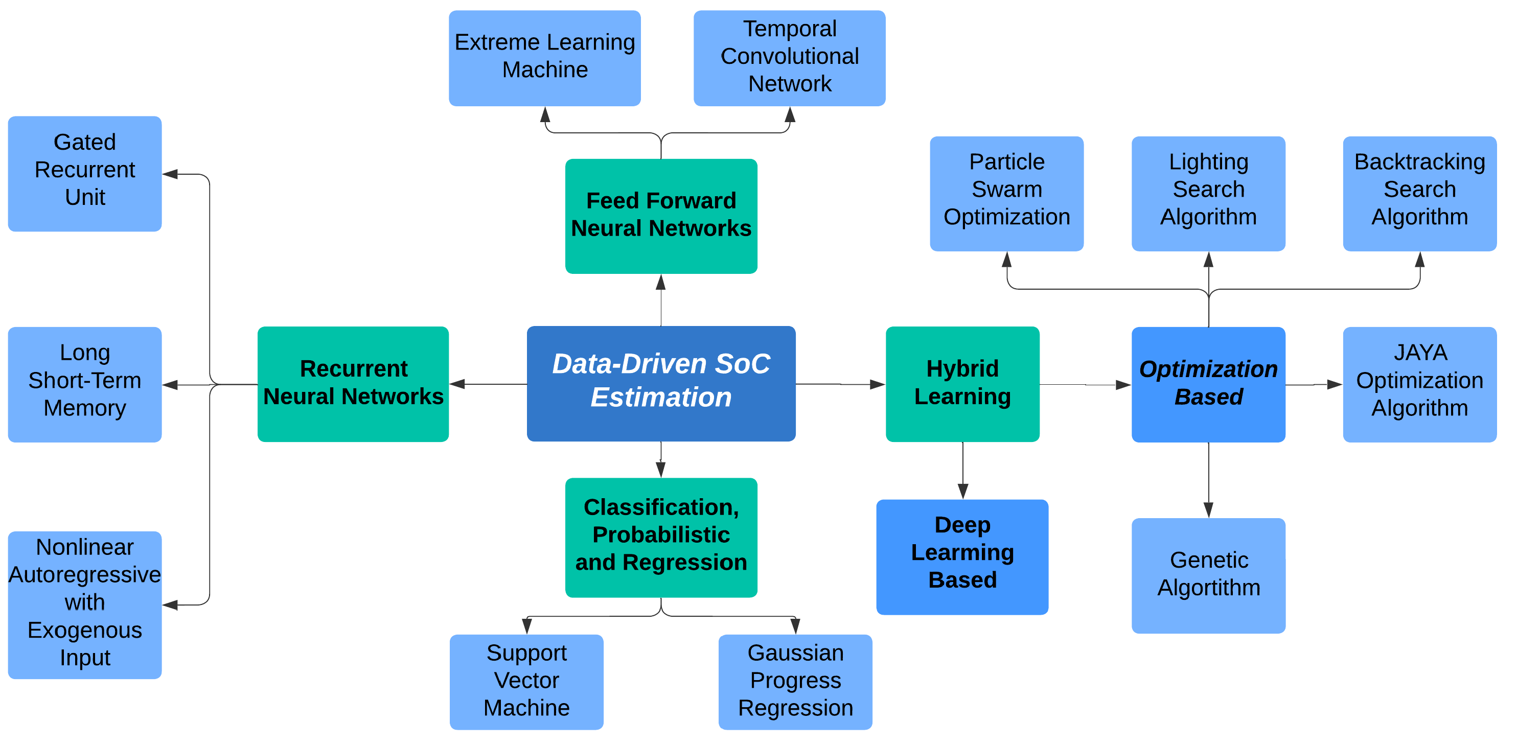
:1. Introduction
2. Classification, Regression, and Probabilistic
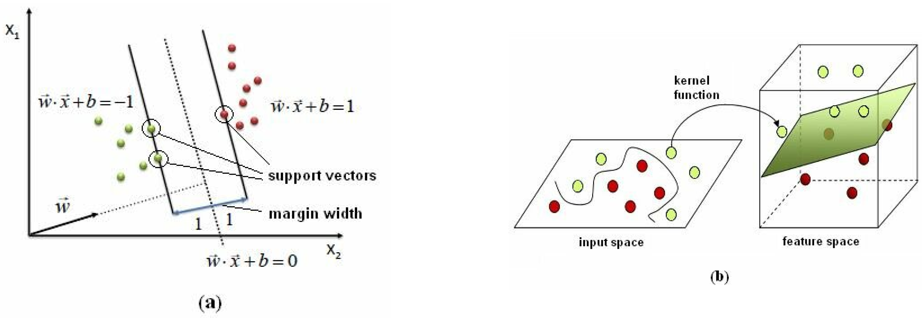
2.1. Support Vector Machine
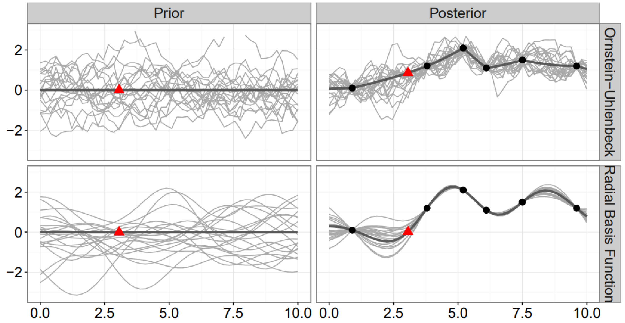
2.2. Gaussian Process Regression
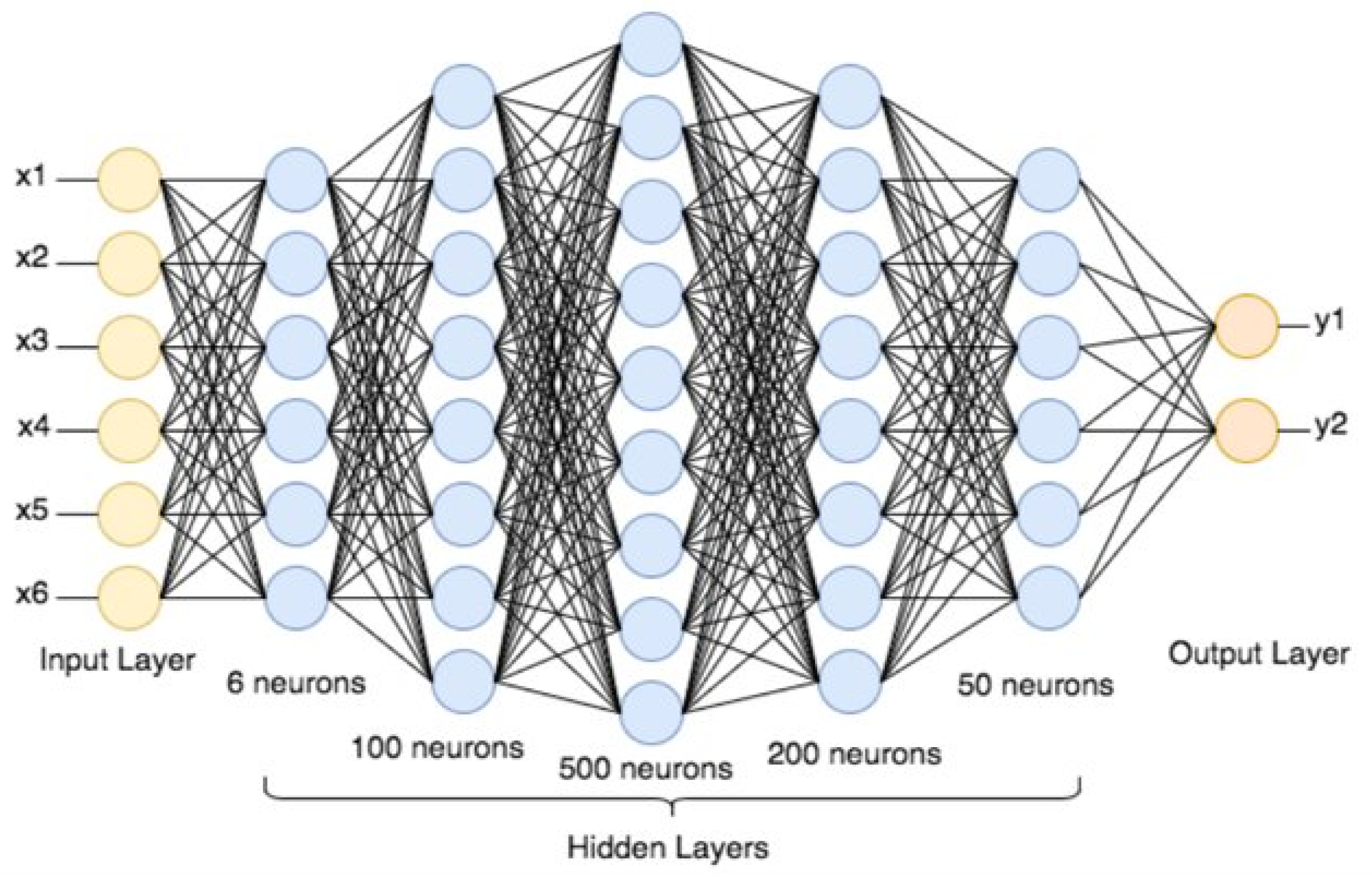
3. Feedforward Neural Network
3.1. Deep Neural Network

| N/N | Ref | Algorithm | Battery | Temperatures | Performance |
|---|---|---|---|---|---|
| 1 | [24] | LS-SVM | 2.2Ah NMC | 25 C | maxError |
| 2 | [26] | GPR | 177Ah NMC | 25 C and 0 C | maxError |
| 3 | [27] | GPR | 2.55 and 2.6Ah LFP | 10 C and 40 C | maxError |
| 4 | [28] | FFNN | 2Ah NCA | −10 C, 0 C, 10 C, and 25 C | maxError |
| 5 | [29] | DNN | 2.9Ah NCA | 20 C, −10 C, 0 C, 10 C, and 25 C | MAE @ 25 C, MAE % @ −20 C |
| 6 | [30] | TCN | 2.9Ah NCA | 0 C, 10 C and 25 C | Average MAE Average RMSE 0.87% |

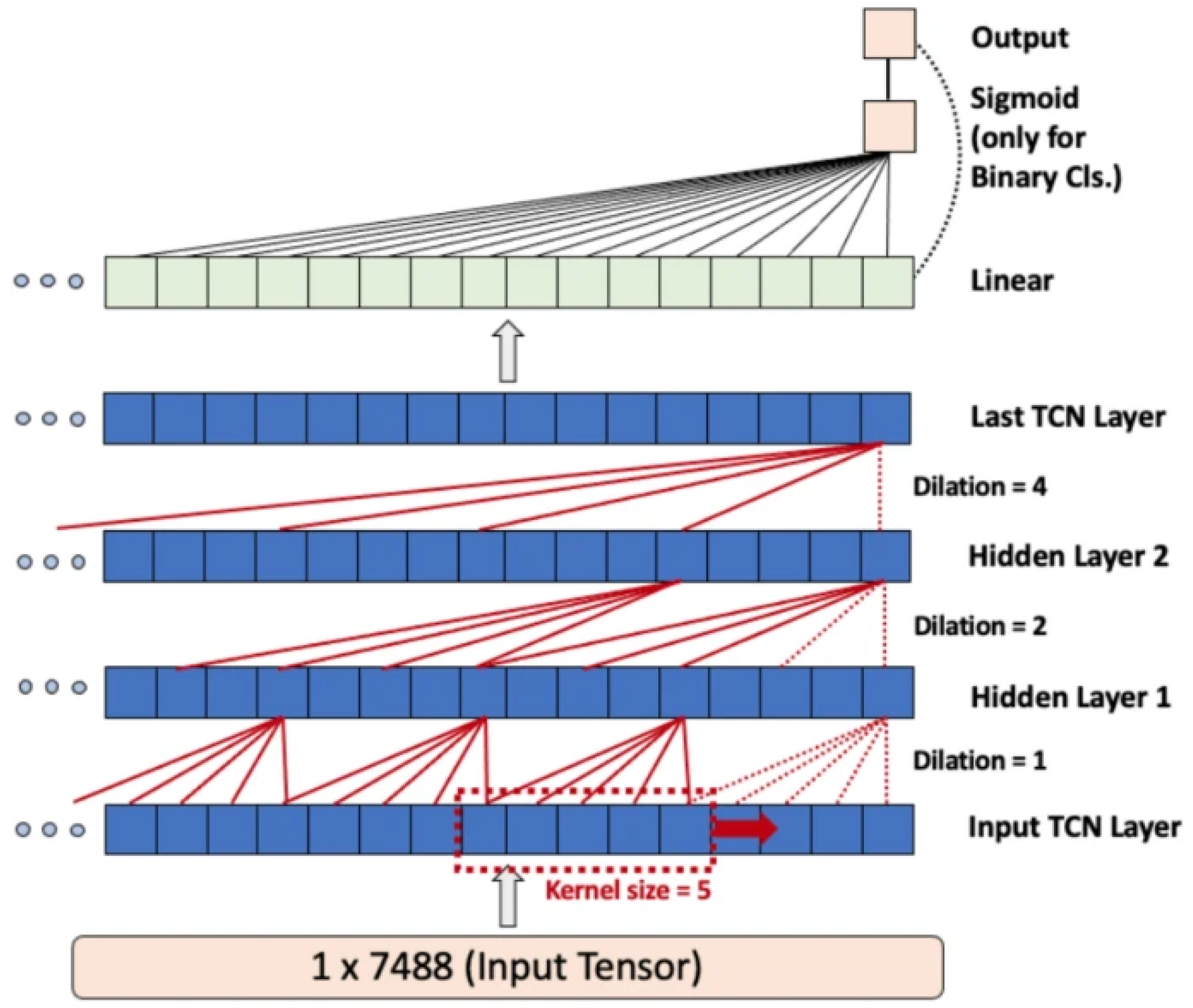
3.2. Temporal Convolutional Network
4. Recurrent Neural Network
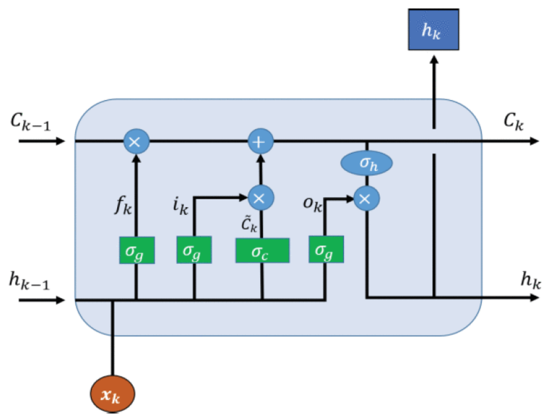
4.1. Long Short-Term Memory Neural Network

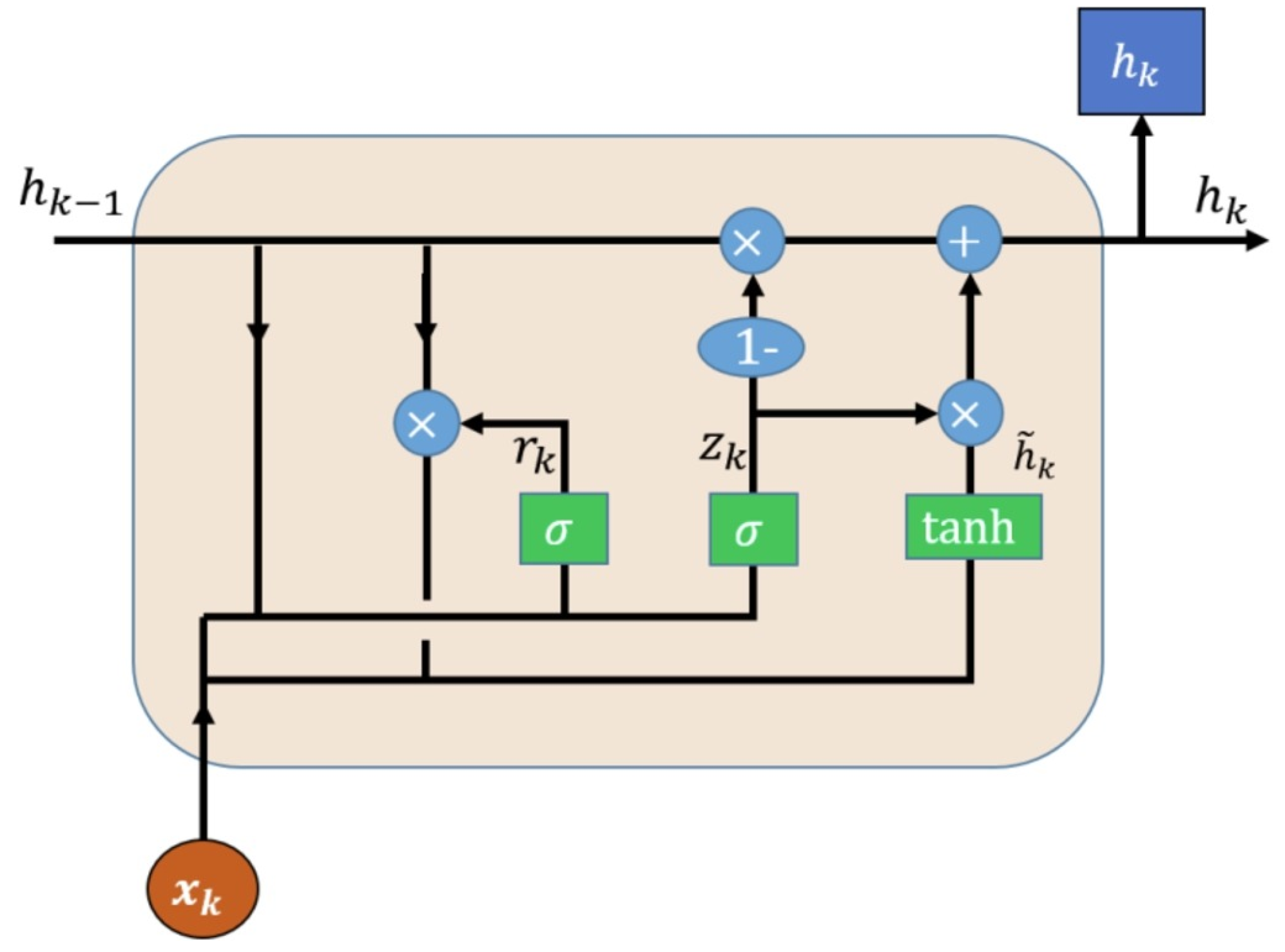
4.2. Gated Recurrent Unit Neural Network
| N/N | Ref | Algorithm | Battery | Temperatures | Performance |
|---|---|---|---|---|---|
| 1 | [33] | LSTM | 2.9Ah NCA | 0 C, 10 C, and 25 C | MAE @ fixed T MAE T: 10 to 25 C |
| 2 | [34] | Stacked LSTM | 1.1Ah LFP | 25 C | RMSE , MAE inaccurate initial SOCs: RMSE , MAE |
| 3 | [35] | LSTM | 2.23Ah LFP [36] | Yes | RMSE , maxError |
| 4 | [37] | LSTM | 1.1Ah LFP | 0 C, 10 C, 20 C, 30 C, and 40 C | RMSE , MAE |
| 5 | [38] | LSTM with Attention | 2.9Ah NCA [39], and 2Ah NMC [36] | Yes | RMSE 1.41% |
| 6 | [40] | Stacked biLSTM | 2.9Ah NCA [39] and 2Ah NMC | Yes | MAEs , @ fixed and varying temperature |
| 7 | [41] |
biLSTM (ED based) | 2.9Ah NCA [39] | Yes | MAE @ varying T |
| 8 | [42] | GRU | 1.3Ah NMC, 1.1Ah LFP | 0 C, 10 C, 20 C, 30 C, 40 C, and 50 C | RMSEs NMC, LFP |
| 9 | [43] | GRU | 2.9Ah NCA [29], 2Ah NMC [36] and 18Ah new | 0 C, 10 C, and 25 C | MAEs , , , resp. |
| 10 | [44] | GRU | 2.2Ah | - | RMSE , MAE |
| 11 | [45] | GRU | 2.3Ah LFP | 0 C, 30 C, and 50 C | RMSE , MAE |
5. Hybrid Learning Approach
5.1. Optimisation-Based Algorithm
| N/N | Ref | Algorithm | Battery | Temperatures | Performance |
|---|---|---|---|---|---|
| 1 | [46] | ELM + GSA | NMC | 25 C and 45 C | RMSE DST, FUDS and US06 |
| 2 | [47] | BPNN + BSA | 2Ah NMC [36] | 0 C, 10 C, and 25 C | RMSE , MAE @ 0 C |
| 3 | [48] | DBN + PSO | 2.2Ah NMC [49] | Yes | AvgError , DST: RMSE , MAE |
| 4 | [50] | NARX + RBFNN + JAYA | LFP | Yes | RMSE , MAE |
| 5 | [51] | RNARX-NN + LSA | 3.2Ah NCA, [36] | 0 C, 25 C and 40 C | RMSE |
| 6 | [52] | NARX-NN + LSA | 2Ah NMC [36] | 0 C, 25 C, and 45 C | RMSE , MAE @ 0 C |
| 7 | [53] | SGAGM | 2.6Ah LC | Yes | MAE less 1% |
5.2. Deep Learning
6. Conclusions
Author Contributions
Funding
Data Availability Statement
Acknowledgments
Conflicts of Interest
Nomenclature
| (SOC) | State of Charge |
| (EOL) | End of Life |
| (ECM) | Equivalent Circuit Model |
| (PF) | Particle Filter |
| (KF) | Kalman Filter |
| (ANN) | Artificial Neural Network |
| (ACKF) | Adaptive Cubature Kalman Filter |
| (EKF) | Extended Kalman Filter |
| (SOH) | State of Health |
| (BMS) | Battery Management System |
| (RNN) | Recurrent Neural Network |
| (LSTM) | Long Short-Term Memory |
| (biLSTM) | Bidirectional Long Short-Term Memory |
| (LIBs) | Lithium-Ion Batteries |
| (CC) | Coulomb Counting |
| (UKF) | Unscented Kalman Filter |
| (GRU) | Gated Recurrent Unit |
| (biGRU) | Bidirectional Gated Recurrent Unit |
| (FC) | Fully Connected |
| (CNN-GRU) | Convolution Gated Recurrent Unit |
| (PSO) | Particle Swarm optimisation |
| (LSA) | Lighting Search Algorithm |
| (GA) | Genetic Algorithm |
| (NARX) | Nonlinear Autoregresive with Exogenous Input |
| (GM) | Grey Model |
| (SGAGM) | Sliding Genetic Algorithm Grey Model |
| (LS-SVM) | Least-Square Support Vector Machine |
| (UPF) | Unscented Particle Filter |
| (LCO) | Lithium Cobalt Oxide |
| (NMC) | Nickel Manganese Cobalt Oxide |
| (LFP) | Lithium Iron Phosphate |
| (MAE) | Mean Absolute Error |
| (RMSE) | Root Mean Squared Error |
| (CALCE) | Centre for Advanced Life Cycle Engineering |
| (UDDS) | Urban Dynamometer Driving Schedule |
| (HWFET) | Highway Fuel Economy Test Cycle |
| (US06) | Highway Driving Schedule |
| (LA92) | California Unified Cycle |
| (DST) | Dynamic Stress Test |
| (FUDS) | Federal Urban Drive Schedule |
| (BJDST) | Beijing Dynamic Stress Test |
| (SVM) | Support Vector Machine |
| (GPR) | Gaussian Process Regression |
| (FFNN) | Feedforward Neural Network |
| (NCA) | Nickel Cobalt Aluminum Oxide |
| (DNN) | Deep Neural Network |
| (TCN) | Temporal Convolutional Network |
| (BSA) | Backtracking Search Algorithm |
| (GSA) | Gravitational Search Algorithm |
| (ELM) | Extreme Learning Machine |
| (BPNN) | Backpropagation Neural Network |
| (RBFNN) | Radial Basis Function Neural Network |
| (GRNN) | Generalised Regression Neural Network |
| (DBN) | Deep Belief Network |
| (RNARX) | Recurrent Nonlinear Autoregressive with Exogenous Inputs |
| (SGAGM) | Sliding Genetic Algorithm Grey Model |
| (GM) | Grey Model |
References
- Yong, J.Y.; Ramachandaramurthy, V.K.; Tan, K.M.; Mithulananthan, N. A review on the state-of-the-art technologies of electric vehicle, its impacts and prospects. Renew. Sustain. Energy Rev. 2015, 49, 365–385. [Google Scholar] [CrossRef]
- Forbes: How Renewables Could Kill off Fossil Fuel Electricity by 2035: New Report. Available online: https://www.forbes.com/sites/davidrvetter/2021/04/26/how-renewables-could-kill-off-fossil-fuel-electricity-by-2035-new-report/?sh=56f63a5565ed/ (accessed on 13 June 2023).
- Blomgren, G.E. The development and future of lithium ion batteries. J. Electrochem. Soc. 2016, 164, A5019–A5025. [Google Scholar] [CrossRef]
- Eleftheriadis, P.; Leva, S.; Gangi, M.; Rey, A.V.; Borgo, A.; Coslop, G.; Groppo, E.; Grande, L.; Sedzik, M. Second life batteries: Current regulatory framework, evaluation methods and economic assessment. In Proceedings of the 2022 IEEE International Conference on Environment and Electrical Engineering and 2022 IEEE Industrial and Commercial Power Systems Europe (EEEIC/I CPS Europe), Prague, Czech Republic, 28 June–1 July 2022. [Google Scholar]
- Rahimi-Eichi, H.; Ojha, U.; Baronti, F.; Chow, M.-Y. Battery management system: An overview of its application in the smart grid and electric vehicles. IEEE Ind. Electron. Mag. 2013, 7, 4–16. [Google Scholar] [CrossRef]
- Eleftheriadis, P.; Leva, S.; Gangi, M.; Rey, A.V.; Groppo, E.; Grande, L. Comparative study of machine learning techniques for the state of health estimation of li-ion batteries. In Proceedings of the 13th Mediterranean Conference on Power Generation, Transmission, Distribution and Energy Conversion (MEDPOWER2022), Valletta, Malta, 7–9 November 2022; pp. 1–6. [Google Scholar]
- Pop, V.; Bergveld, H.J.; Notten, P.H.L.; Regtien, P.P. State-of-the-art of battery state-of-charge determination. Meas. Sci. Technol. 2005, 16, R93. [Google Scholar] [CrossRef]
- Petropoulos, F. Others Forecasting: Theory and practice. Int. J. Forecast. 2022, 38, 705–871. [Google Scholar] [CrossRef]
- Snihir, I.; Rey, W.; Verbitskiy, E.; Belfadhel-Ayeb, A.; Notten, P.H. Battery open-circuit voltage estimation by a method of statistical analysis. J. Power Sources 2006, 159, 1484–1487. [Google Scholar] [CrossRef]
- Ng, K.S.; Moo, C.S.; Chen, Y.P.; Hsieh, Y.C. Enhanced coulomb counting method for estimating state-of-charge and state-of-health of lithium-ion batteries. Appl. Energy 2009, 86, 1506–1511. [Google Scholar] [CrossRef]
- Xiong, R.; Tian, J.; Shen, W.; Sun, F. A novel fractional order model for state of charge estimation in lithium ion batteries. IEEE Trans. Veh. Technol. 2018, 68, 4130–4139. [Google Scholar] [CrossRef]
- Chen, Z.; Sun, H.; Dong, G.; Wei, J.; Wu, J.I. Particle filter-based state-of-charge estimation and remaining-dischargeable-time prediction method for lithium-ion batteries. J. Power Sources 2019, 414, 158–166. [Google Scholar] [CrossRef]
- Zhang, Y.; Xiong, R.; He, H.; Shen, W. Lithium-ion battery pack state of charge and state of energy estimation algorithms using a hardware-in-the-loop validation. IEEE Trans. Power Electron. 2016, 32, 4421–4431. [Google Scholar] [CrossRef]
- Zhong, Q.; Zhong, F.; Cheng, J.; Li, H.; Zhong, S. State of charge estimation of lithium-ion batteries using fractional order sliding mode observer. ISA Trans. 2017, 66, 448–459. [Google Scholar] [CrossRef] [PubMed]
- Lipu, M.; Hannan, M.; Hussain, A.; Ayob, A.; Saad, M.H.; Karim, T.F.; How, D.N. Data-driven state of charge estimation of lithium-ion batteries: Algorithms, implementation factors, limitations and future trends. J. Clean. Prod. 2020, 277, 124110. [Google Scholar] [CrossRef]
- Hannan, M.; Lipu, M.; Hussain, A.; Mohamed, A. A review of lithium-ion battery state of charge estimation and management system in electric vehicle applications: Challenges and recommendations. Renew. Sustain. Energy Rev. 2017, 78, 834–854. [Google Scholar] [CrossRef]
- Xiong, R.; Cao, J.; Yu, Q.; He, H.; Sun, F. Critical review on the battery state of charge estimation methods for electric vehicles. IEEE Access 2018, 6, 1832–1843. [Google Scholar] [CrossRef]
- How, D.N.T.; Hannan, M.A.; Lipu, M.S.H.; Ker, P.J. State of charge estimation for lithium-ion batteries using model-based and data-driven methods: A review. IEEE Access 2019, 7, 136116–136136. [Google Scholar] [CrossRef]
- Wang, Y.; Tian, J.; Sun, Z.; Wang, L.; Xu, R.; Li, M.; Chen, Z. A comprehensive review of battery modeling and state estimation approaches for advanced battery management systems. Renew. Sustain. Energy Rev. 2020, 131, 110015. [Google Scholar] [CrossRef]
- Vidal, C.; Malysz, P.; Kollmeyer, P.; Emadi, A. Machine learning applied to electrified vehicle battery state of charge and state of health estimation: State-of-the-art. IEEE Access 2020, 8, 52796–52814. [Google Scholar] [CrossRef]
- Cui, Z.; Wang, L.; Li, Q.; Wang, K. A comprehensive review on the state of charge estimation for lithium-ion battery based on neural network. Int. J. Energy Res. 2022, 46, 5423–5440. [Google Scholar] [CrossRef]
- Cervantes, J.; Garcia-Lamont, F.; Rodríguez-Mazahua, L.; Lopez, A. A comprehensive survey on support vector machine classification: Applications, challenges and trends. Neurocomputing 2020, 408, 189–215. [Google Scholar] [CrossRef]
- Gokmen, Z.; Elmali, F.; Ozturk, A. Bagging support vector machines for leukemia classification. Int. J. Comput. Sci. Issues (IJCSI) 2012, 9, 355. [Google Scholar]
- Song, Y.; Liu, D.; Liao, H.; Peng, Y. A hybrid statistical data-driven method for on-line joint state estimation of lithium-ion batteries. Appl. Energy 2020, 261, 114408. [Google Scholar] [CrossRef]
- Eric, S.; Speekenbrink, M.; Krause, A. A tutorial on Gaussian process regression with a focus on exploration-exploitation scenarios. BioRxiv 2017. [Google Scholar] [CrossRef]
- Deng, Z.; Hu, X.; Lin, X.; Che, Y.; Xu, L.; Guo, W. Data-driven state of charge estimation for lithium-ion battery packs based on gaussian process regression. Energy 2020, 205, 118000. [Google Scholar] [CrossRef]
- Chen, X.; Chen, X.; Chen, X. A novel framework for lithium-ion battery state of charge estimation based on kalman filter gaussian process regression. Int. J. Energy Res. 2021, 5, 13238–13249. [Google Scholar] [CrossRef]
- Chen, C.; Xiong, R.; Yang, R.; Shen, W.; Sun, F. State-of-charge estimation of lithium-ion battery using an improved neural network model and extended kalman filter. J. Clean. Prod. 2019, 234, 1153–1164. [Google Scholar] [CrossRef]
- Chemali, E.; Kollmeyer, P.J.; Preindl, M.; Emadi, A. State-of-charge estimation of li-ion batteries using deep neural networks: A machine learning approach. J. Power Sources 2018, 400, 242–255. [Google Scholar] [CrossRef]
- Liu, Y.; Li, J.; Zhang, G.; Hua, B.; Xiong, N. State of charge estimation of lithium-ion batteries based on temporal convolutional network and transfer learning. IEEE Access 2021, 9, 34177–34187. [Google Scholar] [CrossRef]
- Meriem, B.; Batouche, M. Deep learning for ligand-based virtual screening in drug discovery. In Proceedings of the 2018 3rd International Conference on Pattern Analysis and Intelligent Systems (PAIS), Tebessa, Algeria, 24–25 September 2018. [Google Scholar]
- Bednarski, B.P.; Singh, A.D.; Zhang, W.; Jones, W.M.; Ramezani, A.N.R. Temporal convolutional networks and data rebalancing for clinical length of stay and mortality prediction. Sci. Rep. 2022, 12, 21247. [Google Scholar] [CrossRef]
- Chemali, E.; Kollmeyer, P.J.; Preindl, M.; Ahmed, R.; Emadi, A. Long short-term memory networks for accurate state-of-charge estimation of li-ion batteries. IEEE Trans. Ind. Electron. 2018, 65, 6730–6739. [Google Scholar] [CrossRef]
- Yang, F.; Song, X.; Xu, F.; Tsui, K.-L. State-of-charge estimation of lithium-ion batteries via long short-term memory network. IEEE Access 2019, 7, 53792–53799. [Google Scholar] [CrossRef]
- Tian, Y.; Lai, R.; Li, X.; Xiang, L.; Tian, J. A combined method for state-of-charge estimation for lithium-ion batteries using a long short-term memory network and an adaptive cubature kalman filter. Appl. Energy 2020, 265, 114789. [Google Scholar] [CrossRef]
- Calce. lithium-Ion Battery Experimental Data. Available online: https://web.calce.umd.edu/batteries/data.htm (accessed on 13 June 2023).
- Yang, F.; Zhang, S.; Li, W.; Miao, Q. State-of-charge estimation of lithium-ion batteries using lstm and ukf. Energy 2020, 201, 117664. [Google Scholar] [CrossRef]
- Mamo, T.; Wang, F.-K. Long short-term memory with attention mechanism for state of charge estimation of lithium-ion batteries. IEEE Access 2020, 8, 94140–94151. [Google Scholar] [CrossRef]
- Kollmeyer, P. Panasonic 18650pf li-ion battery data. Mendeley Data 2018, 1. [Google Scholar] [CrossRef]
- Bian, C.; He, H.; Yang, S. Stacked bidirectional long short-term memory networks for state-of-charge estimation of lithium-ion batteries. Energy 2020, 191, 116538. [Google Scholar] [CrossRef]
- Bian, C.; He, H.; Yang, S.; Huang, T. State-of-charge sequence estimation of lithium-ion battery based on bidirectional long short-term memory encoder-decoder architecture. J. Power Sources 2020, 449, 227558. [Google Scholar] [CrossRef]
- Yang, F.; Li, W.; Li, C.; Miao, Q. State-of-charge estimation of lithium-ion batteries based on gated recurrent neural network. Energy 2019, 175, 66–75. [Google Scholar] [CrossRef]
- Li, C.; Xiao, F.; Fan, Y. An approach to state of charge estimation of lithium-ion batteries based on recurrent neural networks with gated recurrent unit. Energies 2019, 12, 1592. [Google Scholar] [CrossRef]
- Jiao, M.; Wang, D.; Qiu, J. A gru-rnn based momentum optimised algorithm for soc estimation. J. Power Sources 2020, 459, 228051. [Google Scholar] [CrossRef]
- Xiao, B.; Liu, Y.; Xiao, B. Accurate state-of-charge estimation approach for lithium-ion batteries by gated recurrent unit with ensemble optimiser. IEEE Access 2019, 7, 54192–54202. [Google Scholar] [CrossRef]
- Lipu, M.S.H.; Hannan, M.A.; Hussain, A.; Saad, M.H.; Ayob, A.; Uddin, M.N. Extreme learning machine model for state-of-charge estimation of lithium-ion battery using gravitational search algorithm. IEEE Trans. Ind. Appl. 2019, 55, 4225–4234. [Google Scholar] [CrossRef]
- Hannan, M.A.; Lipu, M.S.H.; Hussain, A.; Saad, M.H.; Ayob, A. Neural network approach for estimating state of charge of lithium-ion battery using backtracking search algorithm. IEEE Access 2018, 6, 10069–10079. [Google Scholar] [CrossRef]
- Liu, D.; Li, L.; Song, Y.; Wu, L.; Peng, Y. Hybrid state of charge estimation for lithium-ion battery under dynamic operating conditions. Int. J. Electr. Power Energy Syst. 2019, 110, 48–61. [Google Scholar] [CrossRef]
- Bole, B.; Kulkarni, C.; Daigle, M. Randomized Battery Usage Data Set. 2014. Available online: https://ti.arc.nasa.gov/tech/dash/groups/pcoe/prognostic-data-repository/ (accessed on 13 June 2023).
- Guo, Y.; Yang, Z.; Liu, K.; Zhang, Y.; Feng, W. A compact and optimised neural network approach for battery state-of-charge estimation of energy storage system. Energy 2021, 219, 119529. [Google Scholar] [CrossRef]
- Hannan, M.A.; Lipu, M.S.H.; Hussain, A.; Ker, P.J.; Mahlia, T.M.I.; Mansor, M.; Ayob, A.; Saad, M.H.; Dong, Z.Y. Toward enhanced state of charge estimation of lithium-ion batteries using optimised machine learning techniques. Sci. Rep. 2020, 10, 4687. [Google Scholar] [CrossRef] [PubMed]
- Lipu, M.S.H.; Hannan, M.A.; Hussain, A.; Saad, M.H.M.; Ayob, A.; Blaabjerg, F. State of charge estimation for lithium-ion battery using recurrent narx neural network model based lighting search algorithm. IEEE Access 2018, 6, 28150–28161. [Google Scholar] [CrossRef]
- Chen, L.; Wang, Z.; Lü, Z.; Li, J.; Ji, B.; Wei, H.; Pan, H. A novel state-of-charge estimation method of lithium-ion batteries combining the grey model and genetic algorithms. IEEE Trans. Power Electron. 2018, 33, 8797–8807. [Google Scholar] [CrossRef]
- Saha, B.; Goebel, K. Uncertainty management for diagnostics and prognostics of batteries using bayesian techniques. In Proceedings of the 2008 IEEE Aerospace Conference, Big Sky, MT, USA, 1–8 March 2008; pp. 1–8. [Google Scholar]
- Song, X.; Yang, F.; Wang, D.; Tsui, K.-L. Combined cnn-lstm network for state-of-charge estimation of lithium-ion batteries. IEEE Access 2019, 7, 88894–88902. [Google Scholar] [CrossRef]
- Wei, M.; Ye, M.; Li, J.B.; Wang, Q.; Xu, X. State of charge estimation of lithium-ion batteries using lstm and narx neural networks. IEEE Access 2020, 8, 189236–189245. [Google Scholar] [CrossRef]
- Huang, Z.; Yang, F.; Xu, F.; Song, X.; Tsui, K.-L. Convolutional gated recurrent unit–recurrent neural network for state-of-charge estimation of lithium-ion batteries. IEEE Access 2019, 7, 93139–93149. [Google Scholar] [CrossRef]
- Fasahat, M.; Manthouri, M. State of charge estimation of lithium-ion batteries using hybrid autoencoder and long short term memory neural networks. J. Power Sources 2020, 469, 228375. [Google Scholar] [CrossRef]


| Method | Advantages | Disadvantages |
|---|---|---|
| SVM |
|
|
| GRP |
|
|
| DNN |
|
|
| TCN |
|
|
| LSTM |
|
|
| GRU |
|
|
| Hybrid |
|
|
| N/N | Ref | Algorithm | Battery | Temperatures | Performance |
|---|---|---|---|---|---|
| 23 | [55] | CNN + LSTM | 1.1Ah LFP | 0 C, 10 C, 20 C, 30 C, 40 C and 50 C | maxMAE , maxRMSE and maxMAE , maxRMSE @ varying temp. |
| 24 | [56] | NARX-NN + LSTM | LFP | No | RMSE |
| 25 | [57] | CNN + GRU | 1.3Ah NMC | 0 C, 10 C, 20 C, 26 C, 30 C, 40 C and 50 C | RMSE , MAE @ 0 C |
| 26 | [58] | Autoencoder NN + LSTM | 2Ah NMC [36] | Yes | RMSE , MAE @ 0 C |
Disclaimer/Publisher’s Note: The statements, opinions and data contained in all publications are solely those of the individual author(s) and contributor(s) and not of MDPI and/or the editor(s). MDPI and/or the editor(s) disclaim responsibility for any injury to people or property resulting from any ideas, methods, instructions or products referred to in the content. |
© 2023 by the authors. Licensee MDPI, Basel, Switzerland. This article is an open access article distributed under the terms and conditions of the Creative Commons Attribution (CC BY) license (https://creativecommons.org/licenses/by/4.0/).
Share and Cite
Eleftheriadis, P.; Giazitzis, S.; Leva, S.; Ogliari, E. Data-Driven Methods for the State of Charge Estimation of Lithium-Ion Batteries: An Overview. Forecasting 2023, 5, 576-599. https://doi.org/10.3390/forecast5030032
Eleftheriadis P, Giazitzis S, Leva S, Ogliari E. Data-Driven Methods for the State of Charge Estimation of Lithium-Ion Batteries: An Overview. Forecasting. 2023; 5(3):576-599. https://doi.org/10.3390/forecast5030032
Chicago/Turabian StyleEleftheriadis, Panagiotis, Spyridon Giazitzis, Sonia Leva, and Emanuele Ogliari. 2023. "Data-Driven Methods for the State of Charge Estimation of Lithium-Ion Batteries: An Overview" Forecasting 5, no. 3: 576-599. https://doi.org/10.3390/forecast5030032