Article

Searching for Promisingly Trained Artificial Neural Networks

by
Juan M. Lujano-Rojas
*,
Rodolfo Dufo-López
,
Jesús Sergio Artal-Sevil
and
Eduardo García-Paricio
Department of Electrical Engineering, University of Zaragoza, Calle María de Luna 3, 50018 Zaragoza, Spain
*
Author to whom correspondence should be addressed.
Forecasting 2023, 5(3), 550-575; https://doi.org/10.3390/forecast5030031
Submission received: 3 July 2023 / Revised: 16 August 2023 / Accepted: 1 September 2023 / Published: 4 September 2023
(This article belongs to the Special Issue Advanced Methods for Renewable Energy Forecasting)

Abstract

:
Assessing the training process of artificial neural networks (ANNs) is vital for enhancing their performance and broadening their applicability. This paper employs the Monte Carlo simulation (MCS) technique, integrated with a stopping criterion, to construct the probability distribution of the learning error of an ANN designed for short-term forecasting. The training and validation processes were conducted multiple times, each time considering a unique random starting point, and the subsequent forecasting error was calculated one step ahead. From this, we ascertained the probability of having obtained all the local optima. Our extensive computational analysis involved training a shallow feedforward neural network (FFNN) using wind power and load demand data from the transmission systems of the Netherlands and Germany. Furthermore, the analysis was expanded to include wind speed prediction using a long short-term memory (LSTM) network at a site in Spain. The improvement gained from the FFNN, which has a high probability of being the global optimum, ranges from 0.7% to 8.6%, depending on the forecasting variable. This solution outperforms the persistent model by between 5.5% and 20.3%. For wind speed predictions using an LSTM, the improvement over an average-trained network stands at 9.5%, and is 6% superior to the persistent approach. These outcomes suggest that the advantages of exhaustive search vary based on the problem being analyzed and the type of network in use. The MCS method we implemented, which estimates the probability of identifying all local optima, can act as a foundational step for other techniques like Bayesian model selection, which assumes that the global optimum is encompassed within the available hypotheses.

1. Introduction

Machine learning is central to the ongoing technological advancement. Drawing inspiration from human cognitive and learning processes, the concept behind artificial neural networks (ANNs) was developed. ANNs are essential for forecasting environmental variables, renewable generation, and energy demand, all of which are crucial for effective power management.
Recent studies [1,2] suggest that wind and solar power forecasting techniques can be categorized into image-based approaches, statistical models, machine learning-based techniques, and decomposition-based methods:
  • Image-based methods utilize ground-based systems such as sky cameras, Doppler weather radar systems, LiDAR optical systems, or satellite imagery to predict the cloud cover essential for solar irradiance and power forecasting. Within this category, scientists often incorporate physical models or numerical weather predictions.
  • Statistical models focus on analyzing the intrinsic characteristics of the target time series. Commonly employed methods in this category include the auto-regressive method and its vectorial variant, the Markov chain approach, and the analog ensemble.
  • Machine learning-based techniques encompass methods that employ ANNs, like extreme learning machines or convolutional neural networks, to capture the non-linear characteristics of the variable under prediction. Other techniques in this category include support vector machines, decision trees, and Gaussian processes.
  • Decomposition-based methods cover variational, empirical, and wavelet decompositions, as well as approaches reliant on the Fourier transform.
Furthermore, hybrid models can be developed by merging the aforementioned approaches. Such hybrid strategies can be categorized into stacking-based models and weighted-based techniques. Mixed or combined methods not only pertain to the merging of forecasting techniques but also to how data are handled or pre-processed to enhance prediction outcomes, such as algorithms used for data clustering or feature selection.
Energy demand is another variable for which prediction is highly sought-after. Statistical models, machine learning-based techniques, decomposition-based methods, and their combinations have been successfully applied [3,4]. Additionally, the component estimation technique [5] and the functional data approach [6] have been introduced recently, demonstrating promising results for short- and medium-term electricity demand.
In machine learning methodologies, computer scientists frame the learning process as an optimization problem aimed at minimizing the discrepancy between input and output datasets. This problem is commonly addressed using gradient-based optimization. While most available methodologies offer users a satisfactory solution, they do not guarantee global optimality. In other words, training methods often converge to a solution without definitive knowledge of whether it is a local or global optimum. This uncertainty arises because we lack concrete information about the objective function’s shape under investigation. The challenge of achieving global optimality is intrinsically linked to the struggle algorithms face in moving from a local to a global optimum—a phenomenon termed stagnation around a local optimum. Consequently, the local optimum reached during a specific training attempt of an ANN is influenced by its initially chosen starting point, which is often selected at random.
Training ANNs using heuristic techniques has been proposed as a solution to the stagnation problem. While heuristic techniques can also experience stagnation around local optima [7,8], they explore and exploit the objective function in ways distinct from gradient-based methods. Several researchers have endeavored to enhance the search capabilities of these techniques. Dlugosz and Kolasa [9] examined the Kohonen network and devised a training strategy to circumvent stagnation. Their method analyzes the convergence process by employing the neighborhood radius—a topological parameter that determines how network nodes are considered. They found that the training process stagnates when the neighborhood radius exceeds a certain critical value. Furthermore, they noted an active phase in the training error immediately after the neighborhood radius drops below this value. This active phase is then followed by a stagnation phase, during which the neighborhood radius remains static. The researchers introduced filters on the error signal to eradicate the stagnation phases and implemented a decision mechanism to decrease the neighborhood radius once the active phase concludes. Based on the results, this approach accelerates the training process by a factor of 16 compared to traditional methods, where the neighborhood radius diminishes linearly.
Researchers working with the competitive coevolutionary team-based particle swarm optimizer (CCPSO) have also highlighted concerns regarding stagnation. Scheepers and Engelbrecht [10] conducted an in-depth analysis of the stagnation issue, linking the stagnation phenomenon to the saturation of network weights. To counteract weight saturation, they proposed ensuring that the global best particle’s position remains within the active region of the activation function. This idea is realized by imposing a constraint on the cognitive component of the algorithm. Therefore, a particular particle would update its personal best position only if its current position meets the aforementioned constraint and if this update results in a solution with superior fitness. This adaptation of the CCPSO algorithm prevents the weights from departing from the active region of the activation function, thereby mitigating stagnation. Moreover, the researchers introduced a time-varying perception limit—a variable that diminishes to zero after a specified number of epochs—to encourage better exploitation of available solutions. The team reported encouraging outcomes concerning swarm diversity during the training of a soccer-playing robot team.
Particle swarm optimization (PSO) has been successfully applied to ANN training. Mendes et al. [11] and Gudise and Venayagamoorthy [12] were among the pioneers to demonstrate promising results using PSO. Zhang et al. [13] investigated the characteristics of both backpropagation (BP) and PSO in terms of convergence speed and searching capabilities, leading to a combined approach. While PSO excels in searching for the global optimum, its computational speed is somewhat modest. In contrast, BP rapidly converges to a local minimum, but its capacity to identify the global optimum is limited. Given this backdrop, the authors proposed a hybrid approach leveraging the strengths of both BP and PSO. The methodology involves using PSO to identify a potential global solution, and when optimization begins to stagnate, BP is introduced to refine the local search. Based on a case study analysis, the hybrid BP-PSO method efficiently achieves a high-accuracy trained network compared to either BP or PSO used separately.
Mirjalili et al. [14] integrated the gravitational search algorithm (GSA) with PSO, capitalizing on PSO’s social perspective and GSA’s searching prowess. The combined algorithm was tested on several benchmark problems, successfully navigating around stagnation at local minima. Tarkhaneh and Shen [15] crafted an algorithm that combined PSO operators with the Mantegna Levy distribution to reduce optimization stagnation. Cansu et al. [16] introduced a training algorithm for long short-term memory (LSTM) neural networks, modifying PSO to address the stagnation challenge. Their approach, when compared to the Adam algorithm, displayed promising outcomes. Xue et al. [17] put forward a hybrid gradient descent search algorithm (HGDSA) that explores optimization spaces using gradient descent strategies, subsequently employing BP for localized refinement. Furthermore, HGDSA incorporates a self-adaptive mechanism for strategic selection and updating the learning rate.
The training algorithms’ reliance on random initialization of network parameters introduces a source of uncertainty. This step can significantly influence the local minimum where the training algorithm becomes trapped, a phenomenon intrinsically linked to the training procedure known as procedural variability [18]. Presently, there is a heightened focus on developing a formal approach to address uncertainties in deep neural networks. Typically, uncertainties are categorized as either aleatoric or epistemic. The aleatoric component arises from the intrinsic characteristics of the data under consideration. In contrast, epistemic uncertainty pertains to the absence of knowledge or insufficient information about the model in development [19]. Therefore, the aforementioned procedural variability can be linked to the epistemic facet of uncertainty. Epistemic uncertainty can be quantified through Bayesian and ensemble methods. Bayesian techniques express uncertainty using probability distributions to diminish the generalization error. Conversely, ensemble approaches generate multiple models and a variety of forecasting outcomes, which are then amalgamated to yield a more refined prediction [20,21].
This study seeks to address the following questions:
  • How can scientists accurately estimate local minima during network training?
  • What quantitative advantages are gained by identifying the local minima of the objective function during network training?
  • How do existing training methods in the literature leverage detailed knowledge of the objective function’s local minima?
In relation to the first question, comprehensive access to local minima has received limited attention in the technical literature related to ANN training, especially concerning the probability of identifying them. In our research, we drew upon the work of Finch et al. [22] and employed the Monte Carlo simulation (MCS) approach with a stopping criterion to seek out the local minima of the ANN training optimization problem. Specifically, we repeatedly trained and validated the ANN from various random starting points (RSPs) until a satisfactory probability distribution approximation emerged. Subsequently, we computed the probability of identifying an additional, previously unseen solution (local optimum). This helps determine how comprehensively the local optima have been identified. To our knowledge, this approach to estimating the likelihood of having uncovered all local minima is not commonly employed in ANN training. It ties directly to the aforestated issue of stagnation, the initial point of the training procedure, and is thus linked with epistemic uncertainty.
In relation to the second question, we compare the output derived from using the parameter set, which has a high likelihood of being the global optimum, to the average performance. This comparison allows us to determine the improvement rate over average conditions. This method is applied to various variables of interest, including wind speed, power, and electricity demand.
Lastly, we present a discussion on a comprehensive approach to evaluate the implications of possessing detailed information about the objective function. Specifically, we delve into how the probability of having identified all local minima integrates with existing methodologies. This addresses the third question.
This paper is structured as follows: Section 2 describes the stopping criterion employed and the evaluation of the trained ANN. In Section 3, we present various case studies related to wind speed, power, and load prediction, accompanied by a discussion on robust forecasting. The primary conclusions are outlined in Section 4.

2. Materials and Methods

A typical ANN consists of input, hidden, and output layers, each containing several interconnected units. Feedforward neural networks (FFNNs) and recurrent neural networks (RNNs) with only one hidden layer (often referred to as shallow neural networks) and P units are represented in (1) and (2), respectively. The network operates on a dataset of size T , which considers m = 1 , , M features and q = 1 , , Q outputs. Input and output variables are denoted by the vectors u ( t ) and w ( k , t ) , respectively, as described in (3).
h ( t ) = σ W h x ( k ) × u ( t ) + b h ( k ) w ( k , t ) = σ W y h ( k ) × h ( t ) + b y ( k )
h ( t ) = σ W h h ( k ) × h ( t 1 ) + W h x ( k ) × u ( t ) + b h ( k ) w ( k , t ) = σ W y h ( k ) × h ( t ) + b y ( k )
u ( t ) = u ( t , 1 ) u ( t , m ) u ( t , M ) ;   w ( k , t ) = w ( k , t , 1 ) w ( k , t , q ) w ( k , t , Q )
The structure of an ANN is mathematically represented by matrices, which are dimensioned appropriately based on the number of layers and units. These matrices serve as weighting factors and are determined during the training process. The activation function represented as σ in (1) and (2), adjusts the output values and is typically a sigmoid, hyperbolic tangent, or rectified linear unit function. Equations (1)–(3) describe the input-output relationships for an FFNN and an RNN, respectively. The matrices and vectors W h x ( k ) , W y h ( k ) , W h h ( k ) , b h ( k ) , and b y ( k ) are determined during the training process, which is initialized from various randomly selected points. The index k = 1 , , K refers to each of these starting points.
The practical implementation of an ANN requires training and validation datasets. Combined with a computational procedure or training algorithm, these datasets facilitate the estimation of the weighting factors W h x ( k ) , W y h ( k ) , W h h ( k ) , b h ( k ) , and b y ( k ) . This ensures that the ANN accurately captures the characteristics of the model of interest. The learning capabilities of the trained network are then assessed using an independent dataset, referred to as the testing dataset.
The training process entails solving an optimization problem to minimize the discrepancies between the ANN output and the values from the training dataset. The validation dataset is used to evaluate the network’s generalization capabilities at specific stages of the learning process, helping to prevent overfitting.
Most training methods used to determine the matrices W h x ( k ) , W y h ( k ) , W h h ( k ) , b h ( k ) , and b y ( k ) rely on initial values that are randomly set. These initial values significantly impact the learning process as the resultant solution (i.e., the matrices W h x ( k ) , W y h ( k ) , W h h ( k ) , b h ( k ) , and b y ( k ) ) differs for each initialization point ( k = 1 , , K ). Consequently, these commonly used training methods often find a local minimum. In this work, we conduct an extensive search for local minima using the MCS approach, combined with a stopping criterion to conserve computational resources.
Regarding the stopping criterion for the MCS technique, numerous approaches exist. Ata [23] proposed a strategy that utilizes a user-defined convergence band to increase estimation confidence. Benedetti et al. [24] adopted certain elements from the methodology put forth by Ata. Bayer et al. [25] introduced a stopping methodology that leverages the higher moments of the random variable in question. They observed dependable results, especially in heavy-tailed probability distributions, and effectively circumvented premature convergence.
In this study, we apply the MCS method by sequentially adding batches of a designated size. Define I as the number of Monte Carlo experiments per batch and J as the total number of batches. As a result, the cumulative number of experiments equals I × J . Before utilizing the MCS technique, one must specify:
  • The number of experiments per batch ( I )
  • The total number of batches ( J )
  • The number of discretization bins ( L )
  • The vector to retain the J 1 similarity index values ( s )
  • The tolerance threshold, α .
We determine the cumulative distribution function (CDF) of the targeted random variable by adhering to the subsequent procedure:
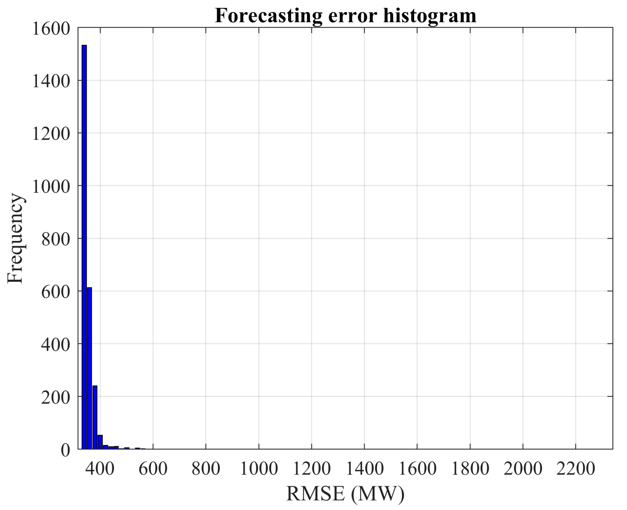
Step 1: Build a matrix ( B ) to specify the seeds belonging to each batch. The seed matrix is B ( i , j ) with I rows ( i = 1 , , I ) and J columns ( j = 1 , , J ). Similarly, create another matrix ( V ) with the same dimensions as B to store the values obtained from the ANN validation process. The root mean square error (RMSE) value obtained from validating the network from the RSP i of the batch j is to be stored in V ( i , j ) . Each RSP is identified by the seed, which is the corresponding value B ( i , j ) .
Step 2: Analyze the first batch by setting j 1 and go to Step 2.1.
Step 2.1: Consider the first seed value by setting i 1 . Go to Step 2.2.
Step 2.2: If i I , go to Step 2.3; else, go to Step 3.
Step 2.3: Train the ANN and store the validation RMSE value in the element V ( i , j ) of the matrix V . Go to Step 2.4.
Step 2.4: Set i i + 1 and go to Step 2.2.
Step 3: Create a column vector ( v a ) with I elements. Then, assign the first column of the matrix V to v a . In other words, assign v a V ( i , j ) with j 1 and i = 1 , , I .
Step 4: Set the stopping variable to zero ( f 0 ). Then, go to Step 5.
Step 5: while f = 0 and j J 1 go to Step 5.1; else, stop.
Step 5.1: Analyze the next batch by setting j j + 1 . Then, go to Step 5.2.
Step 5.2: Consider the first seed value of batch j by setting i 1 . Then, go to Step 5.3.
Step 5.3: If i I go to Step 5.4; else, go to Step 6.
Step 5.4: Train the ANN and store the validation RMSE value in the element V ( i , j ) of the matrix V . Then, go to Step 5.5.
Step 5.5: Set i i + 1 and go to Step 5.3.
Step 6: Build a column vector ( v b ) with j × I elements. This vector is fulfilled with some elements of the matrix V . Reshape the sub-matrix V ( i , m ) with i = 1 , , I and m = 1 , , j into a column vector with j × I elements. Then, store the resulting vector in v b . Go to Step 7.
Step 7: Create a vector ( x ) using the values of v b . The vector x discretizes the interval between the minimum and the maximum observed validation RMSE value until this point. The vector x is built using (4), where x m i n , and x m a x are the minimum and maximum values of v b , and Δ x is the discretization interval with L elements. The vector x is used later to construct the CDF. Once x is obtained, go to Step 8.
x m i n = m i n v b ;   x m a x = m a x ( v b ) x = x m i n , , x m a x   with   step   Δ x = ( x m a x x m i n ) / ( L 1 )
Step 8: Create a column vector with L elements ( y a ). Build the CDF of the vector v a using the intervals of vector x previously determined in Step 7. The corresponding probabilities are assigned to y a . Then, go to Step 9.
Step 9: Create a column vector with L elements ( y b ). Build the CDF of the vector v b using the intervals of vector x previously determined in Step 7. The corresponding probabilities are assigned to y b . Then, go to Step 10.
Step 10: Calculate the Euclidean distance ( d ) between y a and y b according to (5).
d = l = 1 L y a ( l ) y b ( l ) 2
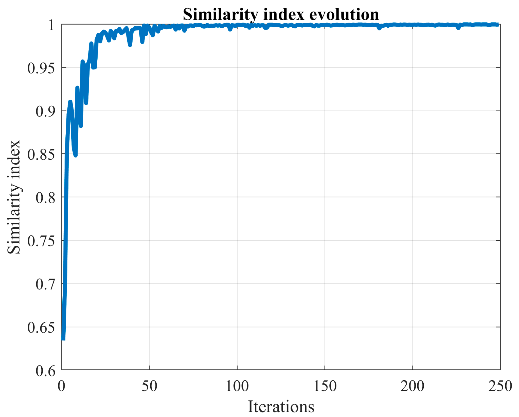
Then, calculate the similarity ( s ( j 1 ) ) between y a and y b using (6).
s ( j 1 ) = 1 1 + d
Once s ( j 1 ) has been calculated, go to Step 11.
Step 11: If the average of the last β -values of the similarity index of (6) is higher than 1 α , assign f 1 and go to Step 5; else, set f 0 , v a v b , and go to Step 5. The parameter α is a tolerance the user sets according to its confidence and reliability requirements.
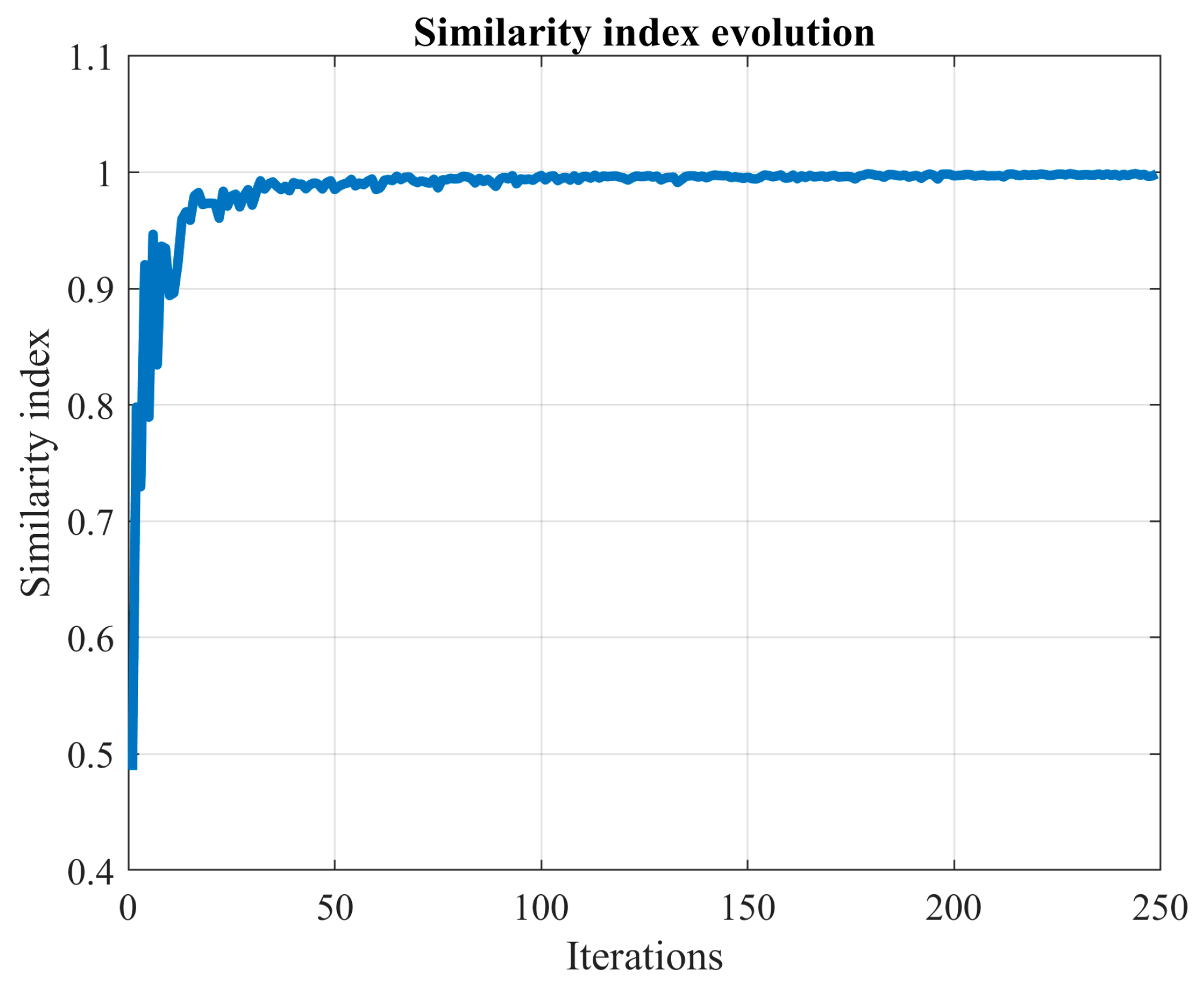
In summary, the stopping rule in this study introduces one batch at a time and gauges the change in the CDF. The MCS process halts when this variation aligns closely with user preferences, as denoted by the parameter α . Instead of relying solely on the CDF variation ( d ), we employ a similarity index ( s ) for enhanced comprehensibility. This index gravitates towards 1 as the MCS advances. Moreover, to mitigate the impact of minor fluctuations on decision-making, we smooth out the similarity index by averaging the last β values. Notably, some researchers address this issue by incorporating a convergence band.
On the one hand, averaging the similarity index over the last β iterations helps in reducing its variability. On the other hand, the factor 1 α , when α is small, primarily serves as a stopping condition. A smaller value of the parameter α indicates a more extended MCS process.
After estimating the probability distribution using an appropriate number of experiments, we can identify the solutions obtained and evaluate them probabilistically. To achieve this, we compute the probability of discovering previously unidentified solutions or species ( Γ ) if the Monte Carlo procedure is repeated once.
The literature has extensively covered this research area [26,27,28,29]. The probability of finding a new solution is contingent upon the number of recently identified local minima. Let x ( l ) and F ( l ) represent the bins and the frequency associated with each bin, respectively, where l = 1 , , L . The number of newly discovered solutions or species ( Ψ ) is determined using (7) [22].
Ψ = l = 1 L ϕ ( l )
where ϕ ( l ) is a function given by (8) [22].
ϕ ( l ) = 1 ;   F ( l ) = 1 0 ;   F ( l ) 1
Then, the probability of finding a new local minimum ( Γ ) is approximated using (9) [22].
Γ = Ψ I × j
The subsequent section demonstrates the implementation of the MCS approach, using the aforementioned stopping criterion, to search for local minima during ANN training for predictive purposes.

3. Results

The MCS approach, along with the stopping criterion described in Section 2, is applied to find an optimal solution for the ANN training problem. In Section 3.1 and Section 3.2, an FFNN is trained and validated multiple times from different RSPs to predict wind power and load demand, respectively. This method enables us to construct a frequency histogram of the forecasting error. From this, we can identify the local minima of the training optimization problem and determine the likelihood of discovering a new solution by extending the MCS approach using (9). Subsequently, in Section 3.3, we repeat this methodology but apply it to an LSTM for wind speed prediction, assessing the advantages of exhaustive search in the training of intricate RNNs. Section 3.4 concludes with a discussion of the Bayesian model selection approach.
Wind power and load demand data are sourced from the transmission systems of the Netherlands and Germany, and they are recorded in 15-min intervals [30,31]. Wind speed data were collected from a meteorological station in Jaca, Spain, and recorded on an hourly basis [32]. Typically, predictions were made one step ahead. Table 1 details the settings used during the implementation of the MCS approach with its stopping criterion.
The FFNN was trained using the Levenberg–Marquardt (LM) algorithm, while the LSTM network utilized the Adam method. Both were executed in MATLAB® on a PC equipped with an Intel Core® i7 CPU, 16 GB RAM, and a 64-bit architecture.

3.1. Short-Term Wind Power Forecasting

We conducted a computational experiment to forecast wind power in 15-min intervals using data from the Netherlands and Germany. For this, we created training, validation, and testing datasets by selecting 30,000 data points starting from 1 January 2022. Figure 1 and Figure 2 depict the sample and partial autocorrelation functions, respectively. Based on these figures, we set the order of the autoregressive neural network to 7, meaning we consider the last seven values to forecast the subsequent one.
The performance of the FFNN, considering up to 50 hidden units, was assessed using the settings from Table 1 and the MCS approach described in the previous section. The minimum, average, and maximum forecasting errors (RMSE) for the validation dataset are depicted in Figure 3. The number of Monte Carlo experiments ranged between 110 and 220.
A noticeable variation in the local maxima can be seen, whereas the average and minimum values stabilize rapidly as more units are added. Based on this data, the optimal number of hidden units, which corresponds to the lowest error (as shown by the ‘Minimum’ in Figure 3), is 30. After conducting 160 experiments, the CDF meets the condition α = 0.05, resulting in a probability ( Γ ) of 4.375%.
From this point forward, we set the number of hidden units to 30 and the stopping tolerance ( α ) to 0. This change in parameters disables the stopping criterion, allowing us to conduct the MCS analysis over 2500 trials, thereby improving accuracy. Figure 4 illustrates the convergence of the LM algorithm for each Monte Carlo experiment. It is evident from the figure that the training process yields valid solutions for each RSP, indicating a successful learning process. The associated histogram showing the number of iterations is depicted in Figure 5. In certain cases, the training process is halted to prevent overfitting; however, more often than not, the maximum number of epochs is attained. Figure 6 presents the value of the similarity index, calculated using (6), to understand the construction of the CDF of the forecasting error.
Lastly, Figure 7 presents the histogram of the forecasting error. Table 2 and Table 3 provide detailed information related to this histogram, including the error from the persistent model, commonly used as a benchmark. In the context of Figure 7 histogram, bins with a frequency greater than one corresponds to identified local minima. Bins with a frequency higher than one represent local minima observed multiple times from different RSPs. Specifically, for Figure 7, 13 local minima were observed with a frequency of one (indicating a unique discovery). Consequently, the probability of identifying a new local minimum would be 13/2500, or 0.52%, as described in (9).
Table 2 reveals that several solutions to the training problem lie within the interval [151.1853 MW, 155.7873 MW]. Table 3 showcases the results derived from evaluating the testing dataset, indicating a 20.3% improvement. Furthermore, the network with the lowest error outperforms a standard network with an average performance of 0.7%.

3.2. Short-Term Load Forecasting

This case study shares several similarities with the one discussed in Section 3.1, with the primary distinction being the analysis of load demand as the variable. Figure 8 and Figure 9 depict the sample and partial autocorrelation functions, respectively. The insights from these figures suggest an autoregressive lag setting of five; this means the last five values are used to forecast the subsequent value. As in the preceding case, we evaluated the FFNN performance for up to 50 hidden units using the configurations outlined in Table 1. Figure 10 presents the minimum, average, and maximum forecasting errors for the validation dataset. The number of Monte Carlo experiments ranged from 70 to 200. An evident trend in the data is the continuous error increase after adding only a few units, which can be attributed to overfitting. Based on these observations, the optimal number of hidden units, as indicated by the lowest error in Figure 10, is five. Additionally, after 180 experiments, the CDF meets the α = 0.05 condition, resulting in a probability ( Γ ) of 12.77%.
Following the procedure outlined in Section 3.1, we set the number of hidden units to 5 and the stopping tolerance to 0, implementing the MCS approach over 2500 realizations. The convergence results are depicted in Figure 11, illustrating how the training process consistently leads to valid solutions for each RSP. In other words, the learning process was executed successfully. The histogram detailing the number of iterations is presented in Figure 12, where we note that the limit of 50 epochs is reached in the majority of instances.
Figure 13 and Figure 14 depict the convergence of the similarity index (as per (6)) and the histogram of forecasting error, respectively. Notably, the highest frequency is centered around the minimum error. Consequently, during a specific Monte Carlo experiment, it is highly likely that the global optimum is attained, as the bin with the lowest error emerges with the highest frequency.
Table 4 and Table 5 provide details related to the histogram of forecasting error (shown in Figure 14), the outcomes of the testing dataset evaluation, and the prediction error resulting from the implementation of the persistent model. Based on this data, employing the MCS approach enables a reduction in the forecasting error by 8.6%, compared to a conventional network with average performance. In comparison to the persistent model, the improvement rate is 5.5%. Notably, the probability of identifying a solution different from those depicted in Figure 14 (bins with a frequency of one or more) stands at 0.48%. As observed in Section 3.1, there are 12 just-discovered local minima (bins with a frequency of one). Hence, the likelihood of uncovering a new local minimum, as per (9), is calculated as 12/2500. To circumvent overfitting (as shown in Figure 12), the training algorithm should terminate prematurely, leading to a significant reduction in computational time, as indicated in Table 4.

3.3. Short-Term Wind Speed Forecasting

In this sub-section, we expand upon the prior analysis by considering both an FFNN and an LSTM neural network, the latter being a type of RNN that is widely used. We examine a wind speed time series from Jaca, a location in Spain, which provides hourly measurements. Figure 15 and Figure 16 illustrate the sample and partial autocorrelation functions. Based on these figures, we determined the number of features in the input dataset to be 23. Additionally, we set the number of hidden units to 25, capped the maximum number of training epochs at 350, and established the stopping tolerance (α) at 0.05. The LSTM network was trained using the Adam algorithm.
Figure 17 and Figure 18 depict the convergence of the training processes for the FFNN and the LSTM network, respectively. Given the LSTM’s more complex structure, its training process necessitates more iterations than the FFNN. The learning process was successfully executed in both instances.
Figure 19 and Figure 20 display histograms of the forecasting error for the FFNN and the LSTM network, respectively. In these histograms, the bins with a frequency of one or higher represent local minima identified during the MCS analysis. For those local minima observed only once (frequency of one), we identified 11 during FFNN training and 25 for the LSTM. Examining Figure 19 and Figure 20, it is evident that the range of values (species) for LSTM training is wider than that of the FFNN. However, the minimum values observed are quite similar.
Table 6 and Table 7 provide detailed information pertaining to these histograms, as well as the results derived from the persistent model. The histogram for the FFNN was constructed based on 200 Monte Carlo realizations, while the histogram for the LSTM network was based on 130 realizations. These values satisfy the stopping criterion with α = 0.05.
Given that the number of experiments for the LSTM network (130 realizations) is fewer than that for the FFNN (200 attempts), and the number of newly discovered solutions is smaller for the FFNN (11 solutions or species) compared to the LSTM network (25 solutions or species), the probability of finding a different solution from those depicted in Figure 19 (5.5%) is less than that in Figure 20 (19.2%). Implementing the MCS improves the average results by 3% using an FFNN and by 9.5% with an LSTM network. In comparison to the persistent model, the FFNN is superior by 6.5%, while the LSTM network provides a 6% lower error.

3.4. Relationship with Bayesian Model Selection

In this section, we discuss the relationship between the MCS and its stopping criterion and the estimation of the probability of observing all local optima ( Γ ) using current methodologies. We place particular emphasis on the method proposed by Oparaji et al. [33]. This method combines Bayesian model selection theory with a model averaging technique to robustly estimate the ANN output.
The method employs a set of hypotheses ( k = 1 , , K ) representing possible values for the ANN parameters. It is posited that these hypotheses denote solutions stagnated in different local optima. (The MCS approach and the probability estimation Γ used in this study can provide a formal foundation for this assumption.) The set of probable values for the ANN parameters, denoted by ψ ( k ) , is mathematically represented by (10).
ψ ( k ) = W h x ( k ) , W y h ( k ) , b h ( k ) , b y ( k )     k = 1 , , K = j × I
It is important to emphasize that the number of hypotheses, K , is determined by the number of Monte Carlo experiments conducted to construct the probability distribution of the forecasting error. Therefore, K = j × I , where j is the value obtained when the condition of Step 11 (the average of the last β -values of the similarity index exceeds 1 α ) is met. Consequently, the index k can be derived by reshaping the matrix B ( i , j ) from Step 1.
Under this framework, Bayesian model selection theory is used to compute the posterior probability of each hypothesis. Specifically, the posterior probability P ψ ( k ) w ¯ ( t )     t = 1 , , T is estimated using (11) as detailed in [33].
P ψ ( k ) w ¯ ( t )     t = 1 , , T = P w ¯ ( t )   t = 1 , , T ψ ( k ) P ψ ( k ) g = 1 K P w ¯ ( t )     t = 1 , , T ψ ( g ) P ψ ( g )
where w ¯ ( t )     t = 1 , , T are the output values of the validation dataset of size T . On the other hand, the prior probability P ψ ( k ) is assumed to follow a uniform distribution so that it is calculated using (12) [33].
P ψ ( k ) = 1 K = 1 j × I
The probability P w ¯ ( t )   t = 1 , , T ψ ( k ) is calculated using (13) and (14) [33] under the assumption that the errors are normally and independently distributed with a mean equal to zero and a determined variance ( θ ( k ) 2 ).
P w ¯ ( t )     t = 1 , , T ψ ( k ) 1 2 π θ ( k ) 2 1 T t = 1 T e x p w ¯ ( t ) w ( k , t ) 2 2 θ ( k ) 2
θ ( k ) 2 = 1 T t = 1 T w ¯ ( t ) w ( k , t ) 2
Then, the model ( k ) to be selected is that with maximum posterior probability (evidence). We identify the hypothesis of the chosen model with the index k ¯ .
After the model has been identified, the subsequent step involves estimating the network’s output values using robust theory. For this purpose, a model averaging technique is employed. Initially, we determine the expected value E A f of the adjustment factor ( A f ) as described in (15) from [33].
E A f = k = 1 K P ψ ( k ) w ¯ ( t )   t = 1 , , T w ( k , t ) w ( k ¯ , t )   t = 1 , , T
where w ( k , t ) is the output value obtained from the network evaluation considering the hypothesis k and the point t of the validation dataset. A similar definition is applied to w ( k ¯ , t ) . These variables can be expressed in vector form using (16) and (17) from [33].
w ( k ) = w ( k , t )     t = 1 , , T
w ( k ¯ ) = w ( k ¯ , t )     t = 1 , , T
The variance of the adjustment factor V A f is calculated using (18) [33].
V A f = k = 1 K P ψ ( k ) w ¯ ( t )   t = 1 , , T w k E w r 2
where the expected value of the robust estimation E w r is calculated using (19) [33].
E w r = w ( k ¯ ) + E A f
And the corresponding variance V w r is obtained from (20) [33].
V w r = V A f
Finally, the confidence interval ( C I ¯ and C I _ ) related to the network output is estimated by using (21) and (22) [33].
C I ¯ = E w r + 1.96 V w r
C I _ = E w r 1.96 V w r
For illustrative purposes, Oparaji et al. [33] use the Ishigami function as a benchmark for their method. In this study, we have also explored this case using an FFNN; the specific settings are detailed in Table 8.
Figure 21 displays the histogram of evaluation errors over the validation dataset for the case based on the Ishigami function. As previously mentioned, bins with a frequency equal to or higher than one represent the local minima discovered. Figure 22 depicts the posterior probability value (as derived from (10)–(14)) for each of the 2500 hypotheses. The hypothesis with the most promising behavior is number 118 ( k ¯ =118). Finally, Figure 23 presents the robust output (as per (15)–(22)) of the FFNN when considering the validation dataset.
In relation to the cases analyzed in Section 3.1,Section 3.2, Section 3.3, Figure 24, Figure 25, Figure 26 and Figure 27 present the calculation of posterior probability for each, as outlined in (10)–(14). These data are complemented by Table 9, which reports the selected hypothesis ( k ¯ ) for each case, the tolerance ( α ), and the associated probability of discovering new local optima ( Γ ).
It is worth noting that in all the case studies, the hypothesis with the lowest error also had the highest evidence (posterior probability).
The probability of discovering a new local optimum is of paramount importance. In the forecasting of hourly wind speed using an FFNN (as discussed in Section 3.3), we set the parameter α of the stopping criterion to 0.05, executing 200 Monte Carlo experiments with a probability ( Γ ) of 5.5%. Adjusting α to 0.01 yields the values presented in Table 10.
We observe that the number of Monte Carlo experiments rises to 590, and the promising hypothesis ( k ¯ ) shifts to 400. Meanwhile, the probability of discovering a new local optimum decreases to 2.54%. Even with a low probability ( Γ ), we can identify a promising solution, but this comes at the cost of significant computational resources—in this instance, increasing the number of Monte Carlo experiments from 200 to 590.

4. Conclusions

This paper employs the Monte Carlo simulation technique coupled with a stopping criterion to construct the probability distribution of the learning error for an ANN used in short-term forecasting. In essence, the learning process (LM for FFNN and Adam for LSTM network) initiates from a distinct point for each Monte Carlo realization, aiming to identify the local minima. Subsequently, we estimate the probability of discovering a new local minimum if the Monte Carlo process were extended.
We applied this procedure to wind power, load demand, and wind speed time series from various European locations. The enhancement gained from a thorough search of an FFNN with superior performance, when compared to an average trained network, is 0.7% for wind power prediction, 8.6% for load demand forecasting, and 3% for wind speed prediction. Moreover, when using an LSTM network—a type of recurrent neural network—for wind speed prediction, the improvement rate rises to 9.5%.
The FFNN, when trained exhaustively, delivers a performance that is 20.3% better than the persistent model for wind power forecasting, 5.5% for load demand prediction, and 6.5% for wind speed forecasting. When predicting wind speed using an LSTM, the performance improves by 6% compared to the persistent approach.
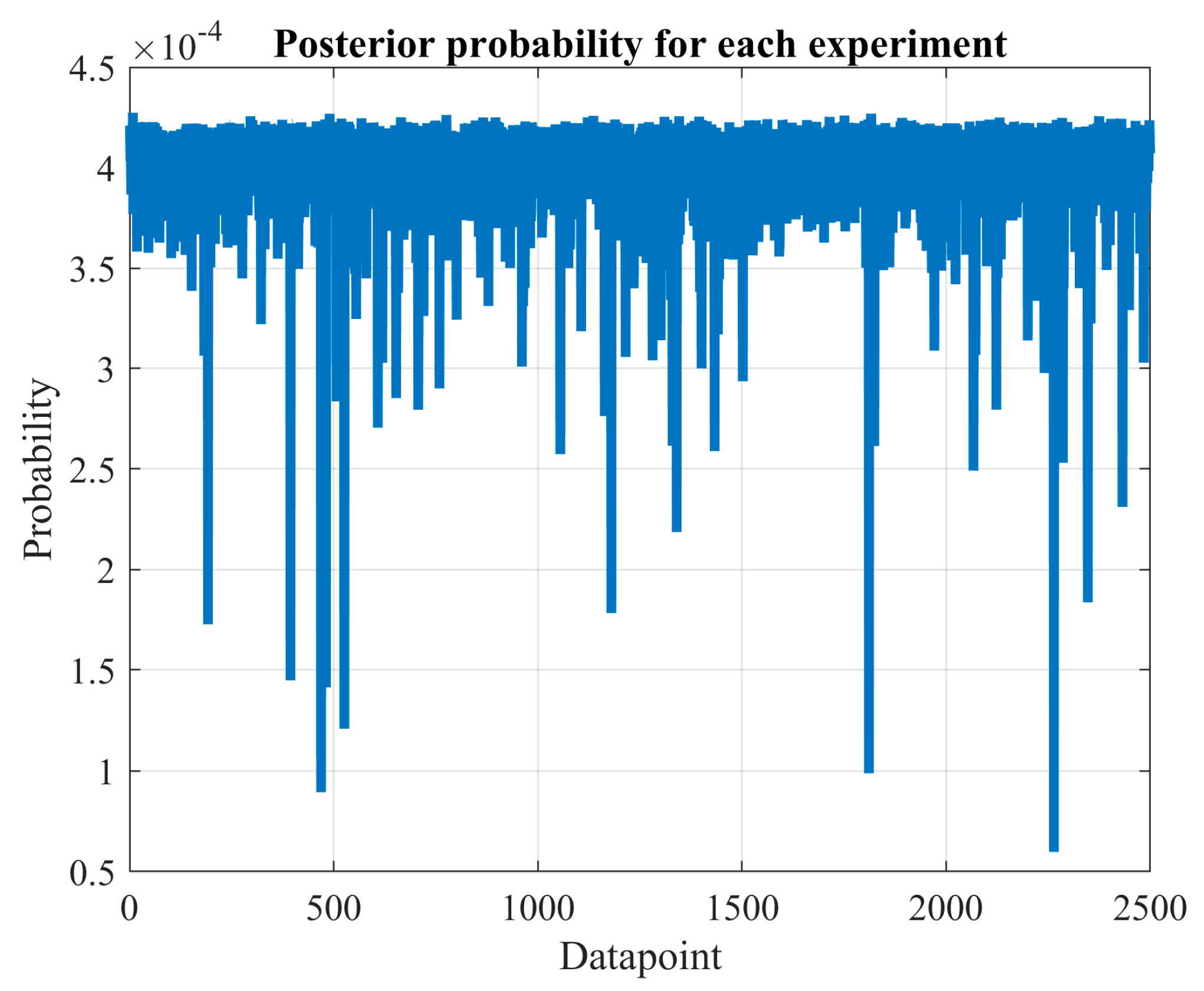
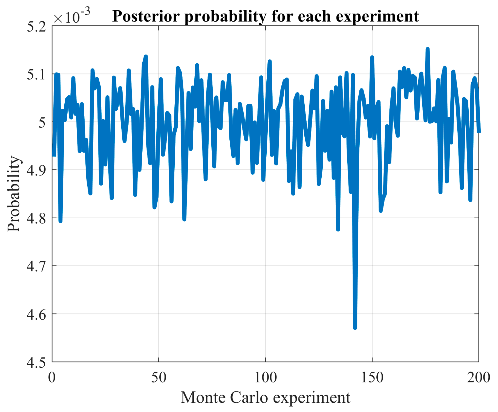
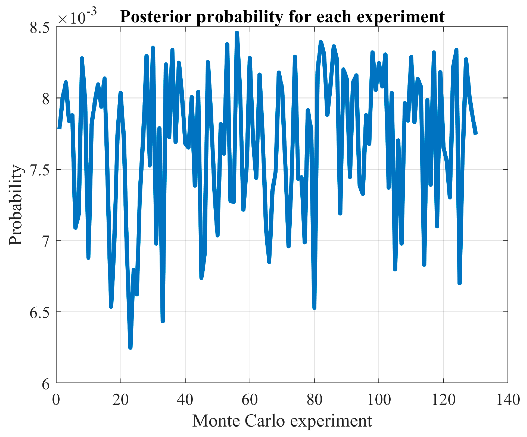
These results indicate that the advantages of exhaustive search vary significantly based on the problem being analyzed and the specific network type used. By increasing the number of Monte Carlo experiments, the confidence in the observed solutions is bolstered. For instance, the probability of discovering a new local optimum drops significantly in the cases of wind power and load demand when the number of experiments is increased. Specifically, for wind power prediction, it drops from 4.375% with 160 experiments to 0.52% with 2500 experiments. Similarly, for load demand forecasting, the decline is from 12.77% with 160 experiments to 0.48% with 2500 experiments.
Based on the results presented in Figure 3 and Figure 10, the network trained for load demand forecasting appears more susceptible to overfitting compared to the one used for wind power prediction.
The MCS method introduced in this study can be utilized to formally validate the assumption of accessing all local optima used in Bayesian theory for model selection. This was demonstrated in Section 3.4, where the hypothesis with the lowest error consistently exhibited the most promising evidence.
In future work, parallel computing can be employed to decrease the computational time required. Additionally, a more precise estimation of the probability of discovering an unseen solution ( Γ ) can be explored. Other neural network architectures might also be considered.

Author Contributions

Conceptualization, J.M.L.-R. and R.D.-L.; methodology, J.M.L.-R.; software, J.M.L.-R.; validation, E.G.-P.; formal analysis, J.S.A.-S.; investigation, E.G.-P.; resources, J.S.A.-S.; data curation, J.S.A.-S.; writing—original draft preparation, J.M.L.-R.; writing—review and editing, R.D.-L.; visualization, E.G.-P.; supervision, R.D.-L.; project administration, R.D.-L.; funding acquisition, R.D.-L. All authors have read and agreed to the published version of the manuscript.

Funding

This work was supported by the Spanish Government (Ministerio de Ciencia e Innovación, Agencia Estatal de Investigación) and by the European Union/European Regional Development Fund [Grant PID2021-123172OB-I00 funded by MCIN/AEI/ 10.13039/501100011033 and by “ERDF A way of making Europe”]; [Grant TED2021-129801B-I00 funded by MCIN/AEI/ 10.13039/501100011033 and by European Union NextGenerationEU/PRTR].

Conflicts of Interest

The authors declare no conflict of interest.

References

  1. Tawn, R.; Browell, J. A review of very short-term wind and solar power forecasting. Renew. Sustain. Energy Rev. 2022, 153, 111758. [Google Scholar] [CrossRef]
  2. Wang, Y.; Zou, R.; Liu, F.; Zhang, L.; Liu, Q. A review of wind speed and wind power forecasting with deep neural networks. Appl. Energy 2021, 304, 117766. [Google Scholar] [CrossRef]
  3. Lago, J.; Marcjasz, G.; De Schutter, B.; Weron, R. Forecasting day-ahead electricity prices: A review of state-of-the-art algorithms, best practices and an open-access benchmark. Appl. Energy 2021, 293, 116983. [Google Scholar] [CrossRef]
  4. Nowotarski, J.; Weron, R. Recent advances in electricity price forecasting: A review of probabilistic forecasting. Renew. Ad Sustain. Energy Rev. 2018, 81, 1548–1568. [Google Scholar] [CrossRef]
  5. Shah, I.; Iftikhar, H.; Ali, S. Modeling and forecasting medium-term electricity consumption using component estimation technique. Forecasting 2020, 2, 9. [Google Scholar] [CrossRef]
  6. Shah, I.S.; Jan, F.H.; Ali, S. Functional data approach for short-term electricity demand forecasting. Math. Probl. Eng. 2022, 2022, 6709779. [Google Scholar] [CrossRef]
  7. Schmitt, M.; Wanka, R. Particle swarm optimization almost surely finds local optima. Theor. Comput. Sci. 2015, 561, 57–72. [Google Scholar] [CrossRef]
  8. Raß, A.; Schmitt, M.; Wanka, R. Explanation of stagnation at points that are not local optima in particle swarm optimization by potential analysis. In Proceedings of the 2015 Annual Conference on Genetic and Evolutionary Computation, Madrid, Spain, 11–15 July 2015; Silva, S., Ed.; Association for Computing Machinery: New York, NY, USA, 2015. [Google Scholar] [CrossRef]
  9. Dlugosz, R.; Kolasa, M. New fast training algorithm suitable for hardware Kohonen neural networks designed for analysis of biomedical signals. In Proceedings of the 2nd International Conference on Biomedical Electronics and Devices, Oporto, Portugal, 14–17 January 2009; Filho, T.F.B., Gamboa, H., Eds.; INSTICC-Institute for Systems and Technologies of Information, Control and Communication: Setubal, Portugal, 2009. [Google Scholar]
  10. Scheepers, C.; Engelbrecht, A.P. Analysis of stagnation behavior of competitive coevolutionary trained neuro-controllers. In Proceedings of the 2014 IEEE Symposium on Swarm Intelligence (SIS), Orlando, FL, USA, 9–12 December 2014; IEEE: New York, NY, USA, 2014. [Google Scholar]
  11. Mendes, R.; Cortez, P.; Rocha, M.; Neves, J. Particle swarms for feedforward neural network training. In Proceedings of the 2002 International Joint Conference on Neural Network, Honolulu, HI, USA, 12–18 May 2002; IEEE: New York, NY, USA, 2002; Volume 1–3. [Google Scholar]
  12. Gudise, V.G.; Venayagamoorthy, G.K. Comparison of particle swarm optimization and backpropagation as training algorithms for neural networks. In Proceedings of the 2003 IEEE Swarm Intelligence Symposium (SIS 03), Indianapolis, IN, USA, 24–16 April 2003; IEEE: New York, NY, USA, 2003. [Google Scholar]
  13. Zhang, J.R.; Zhang, J.; Lok, T.M.; Lyu, M.R. A hybrid particle swarm optimization-back-propagation algorithm for feedforward neural network training. Appl. Math. Comput. 2007, 185, 1026–1037. [Google Scholar] [CrossRef]
  14. Mirjalili, S.; Hashim, S.Z.M.; Sardroudi, H.M. Training feedforward neural networks using hybrid particle swarm optimization and gravitational search algorithm. Appl. Math. Comput. 2012, 218, 11125–11137. [Google Scholar] [CrossRef]
  15. Tarkhaneh, O.; Shen, H.F. Training of feedforward neural networks for data classification using hybrid particle swarm optimization, Mantegna Levy flight and neighborhood search. Helyion 2019, 5, e01275. [Google Scholar] [CrossRef]
  16. Cansu, T.; Kolemen, E.; Karahasan, O.; Bas, E.; Egrioglu, E. A new training algorithm for long short-term memory artificial neural network based on particle swarm optimization. In Granular Computing; Springer: Berlin/Heidelberg, Germany, 2023. [Google Scholar] [CrossRef]
  17. Xue, Y.; Tong, Y.L.; Neri, F. A hybrid training algorithm based on gradient descent and evolutionary computation. In Applied Intelligence; Springer: Berlin/Heidelberg, Germany, 2023. [Google Scholar] [CrossRef]
  18. Huang, Z.; Lam, H.; Zhang, H. Quantifying Epistemic Uncertainty in Deep Learning. arXiv 2023, arXiv:2110.12122. [Google Scholar] [CrossRef]
  19. Abdar, M.; Pourpanah, F.; Hussain, S.; Rezazadegan, D.; Liu, L.; Ghavamzadeh, M.; Fieguth, P.; Cao, X.C.; Khosravi, A.; Acharya, U.R.; et al. A review of uncertainty quantification in deep learning: Techniques, applications and challenges. Inf. Fusion 2021, 76, 243–297. [Google Scholar] [CrossRef]
  20. Zhou, X.L.; Liu, H.; Pourpanah, F.; Zeng, T.Y.; Wang, X.Z. A survey on epistemic (model) uncertainty in supervised learning: Recent advances and applications. Neurocomputing 2022, 489, 449–465. [Google Scholar] [CrossRef]
  21. Gawlikowski, J.; Tassi, C.R.N.; Ali, M.; Lee, J.; Humt, M.; Feng, J.; Kruspe, A.; Triebel, R.; Jung, P.; Roscher, R.; et al. A survey of uncertainty in deep neural networks. In Artificial Intelligence Review; Springer: Berlin/Heidelberg, Germany, 2023. [Google Scholar] [CrossRef]
  22. Finch, S.J.; Mendell, N.R.; Thode, H.C.J. Probabilistic measures of adequacy of a numerical search for a global maximum. J. Am. Stat. Assoc. 1989, 84, 1020–1023. [Google Scholar] [CrossRef]
  23. Ata, M. A convergence criterion for the Monte Carlo estimates. Simul. Model. Pract. Theory 2007, 15, 237–246. [Google Scholar] [CrossRef]
  24. Benedetti, L.; Claeys, F.; Nopens, I.; Vanrolleghem, P.A. Assessing the convergence of LHS Monte Carlo simulations of wastewater treatment models. Water Sci. Technol. 2011, 63, 2219–2224. [Google Scholar] [CrossRef]
  25. Bayer, C.; Hoel, H.; von Schwerin, E.; Tempone, R. On nonasymptotic optimal stopping criteria in Monte Carlo simulations. SIAM J. Sci. Comput. 2014, 36, A869–A885. [Google Scholar] [CrossRef]
  26. Starr, N. Linear estimation of the probability of discovering a new species. Ann. Stat. 1979, 7, 644–652. [Google Scholar] [CrossRef]
  27. Mao, C.X. Predicting the conditional probability of discovering a new class. J. Am. Stat. Assoc. 2004, 99, 1108–1118. [Google Scholar] [CrossRef]
  28. Lijoi, A.; Mena, R.H.; Prünster, I. Bayesian nonparametric estimation of the probability of discovering new species. Biometrika 2007, 94, 769–786. [Google Scholar] [CrossRef]
  29. Blatt, D.; Hero, A.O. On tests for global maximum of the log-likelihood function. IEEE Trans. Inf. Theory 2007, 53, 2510–2525. [Google Scholar] [CrossRef]
  30. Actual and Forecasted Wind Energy Feed-In. Available online: https://netztransparenz.tennet.eu/electricity-market/transparency-pages/transparency-germany/network-figures/actual-and-forecast-wind-energy-feed-in/ (accessed on 2 July 2023).
  31. Annual Peak Load and Load Curve. Available online: https://netztransparenz.tennet.eu/electricity-market/transparency-pages/transparency-germany/network-figures/annual-peak-load-and-load-curve/ (accessed on 2 July 2023).
  32. State Meteorological Agency (AEMET). Available online: https://www.aemet.es/en/portada (accessed on 2 July 2023).
  33. Oparaji, U.; Sheu, R.J.; Bankhead, M.; Austin, J. Robust artificial neural network for reliability and sensitivity analyses of complex non-linear systems. Neural Netw. 2017, 96, 80–90. [Google Scholar] [CrossRef] [PubMed]
Figure 1. Autocorrelation function (wind power time series).
Forecasting 05 00031 g001
Figure 2. Partial autocorrelation function (wind power time series).
Forecasting 05 00031 g002
Figure 3. Validation error for different network configurations (wind power prediction with FFNN).
Forecasting 05 00031 g003
Figure 4. Convergence analysis for each RSP (wind power prediction with FFNN).
Forecasting 05 00031 g004
Figure 5. Frequency histogram of training iterations (wind power prediction with FFNN).
Forecasting 05 00031 g005
Figure 6. The behavior of the similarity index (wind power prediction with FFNN).
Forecasting 05 00031 g006
Figure 7. Frequency histogram of forecasting error (wind power prediction with FFNN).
Forecasting 05 00031 g007
Figure 8. Autocorrelation function (load demand time series).
Forecasting 05 00031 g008
Figure 9. Partial autocorrelation function (load demand time series).
Forecasting 05 00031 g009
Figure 10. Validation error for different network configurations (load prediction with FFNN).
Forecasting 05 00031 g010
Figure 11. Convergence analysis for each RSP (load prediction with FFNN).
Forecasting 05 00031 g011
Figure 12. Frequency histogram of training iterations (load prediction with FFNN).
Forecasting 05 00031 g012
Figure 13. Convergence of the similarity index (load prediction with FFNN).
Forecasting 05 00031 g013
Figure 14. Frequency histogram of forecasting error (load prediction with FFNN).
Forecasting 05 00031 g014
Figure 15. Autocorrelation function (wind speed time series).
Forecasting 05 00031 g015
Figure 16. Partial autocorrelation function (wind speed time series).
Forecasting 05 00031 g016
Figure 17. Convergence for the FFNN (wind speed prediction with FFNN).
Forecasting 05 00031 g017
Figure 18. Convergence for the LSTM (wind speed prediction with LSTM).
Forecasting 05 00031 g018
Figure 19. Frequency histogram of forecasting error for FFNN (wind speed prediction with FFNN).
Forecasting 05 00031 g019
Figure 20. Frequency histogram of forecasting error for LSTM (wind speed prediction with LSTM).
Forecasting 05 00031 g020
Figure 21. Frequency histogram of FFNN evaluation error (Ishigami function).
Forecasting 05 00031 g021
Figure 22. Posterior probability (Ishigami function).
Forecasting 05 00031 g022
Figure 23. Robust FFNN output (Ishigami function).
Forecasting 05 00031 g023
Figure 24. Posterior probability (wind power prediction with FFNN).
Forecasting 05 00031 g024
Figure 25. Posterior probability (load demand prediction with FFNN).
Forecasting 05 00031 g025
Figure 26. Posterior probability (wind speed prediction with FFNN).
Forecasting 05 00031 g026
Figure 27. Posterior probability (wind speed prediction with LSTM).
Forecasting 05 00031 g027
Table 1. Parameters of stopping criterion and dataset description.
ParameterValue
Maximum number of training epochs50
Learning rate0.001
Number of experiments per batch ( I )10
Number of batches ( J )250
Stopping tolerance ( α )0.05
Autoregressive smoothing order ( β )3
Number of discretization bins ( L )100
Size of wind power and load training dataset10,000
Size of wind power and load validation dataset10,000
Size of wind power and load testing dataset10,000
Size of wind speed training dataset4335
Size of wind speed validation dataset2165
Size of wind speed testing dataset2165
Table 2. Performance over the validation dataset for wind power forecasting.
ParameterValue
Number of hidden units30
Minimum RMSE (MW)151.1853
Average RMSE (MW)152.1854
Maximum RMSE (MW)155.7873
Probability ( Γ )13/2500
Computational Time (HH:MM:SS)01:51:01
Persistent RMSE (MW)196.9942
Table 3. Performance over the testing dataset for wind power forecasting.
ParameterValue
RMSE (MW)160.9722
Persistent RMSE (MW)202.0250
Table 4. Performance over the validation dataset for load demand forecasting.
ParameterValue
Number of hidden units5
Minimum RMSE (MW)329.3708
Average RMSE (MW)360.1873
Maximum RMSE (MW)2326.8992
Probability ( Γ )12/2500
Computational Time (HH:MM:SS)00:14:46
Persistent RMSE (MW)347.5793
Table 5. Performance over the testing dataset for load demand forecasting.
ParameterValue
RMSE (MW)323.6091
Persistent RMSE (MW)342.3337
Table 6. Performance over the validation dataset for wind speed forecasting.
ParameterValue
Number of hidden units25
Network typeFFNNLSTM
Minimum RMSE (m/s)1.06351.0687
Average RMSE (m/s)1.09691.1808
Maximum RMSE (m/s)1.19961.4474
Probability ( Γ )11/20025/130
Computational Time (HH:MM:SS)00:02:1304:36:56
Persistent RMSE (m/s)1.1814
Table 7. Performance over the testing dataset for wind speed forecasting.
ParameterValue
Network typeFFNNLSTM
RMSE (m/s)1.00501.0104
Persistent RMSE (m/s)1.0745
Table 8. Parameters and dataset description for Ishigami function-based case.
ParameterValue
Maximum number of training epochs50
Learning rate0.001
Number of experiments per batch ( I )10
Number of batches ( J )250
Stopping tolerance ( α )0
Autoregressive smoothing order ( β )3
Number of discretization bins ( L )100
Size of training dataset100
Size of validation dataset100
Size of testing dataset100
Table 9. Summary of hypotheses selected and their associated probability.
Case Hypothesis   ( k ¯ ) α Probability   ( Γ )
Ishigami function (FFNN)11800.004
Wind power forecasting (FFNN)3900.0052
Load demand forecasting (FFNN)800.0048
Wind speed (FFNN)1760.050.055
Wind speed (LSTM)560.050.1923
Table 10. Results obtained from reducing α to 0.01 during wind speed prediction with FFNN.
Case Hypothesis   ( k ¯ ) α Probability   ( Γ )
Wind speed (FFNN)1760.050.055
Wind speed (FFNN)4000.010.0254
Disclaimer/Publisher’s Note: The statements, opinions and data contained in all publications are solely those of the individual author(s) and contributor(s) and not of MDPI and/or the editor(s). MDPI and/or the editor(s) disclaim responsibility for any injury to people or property resulting from any ideas, methods, instructions or products referred to in the content.

