Soil Degradation Mapping in Drylands Using Unmanned Aerial Vehicle (UAV) Data


Abstract
:
1. Introduction
2. Materials and Methods
2.1. Study Site
2.2. Field Mapping
2.3. Land Cover Mapping
2.4. Accuracy Assessment
- i—class number
- N—total number of classified values compared to reference values
- mi,i—number of values belonging to reference class I that have also been classified as class i
- Ci—total number of predicted (classified) values belonging to class i
- R—total number of reference values belonging to class i
2.5. Landscape Unit (LU) Mapping
2.6. Incorporating Terrain Attributes in LU Mapping
3. Results
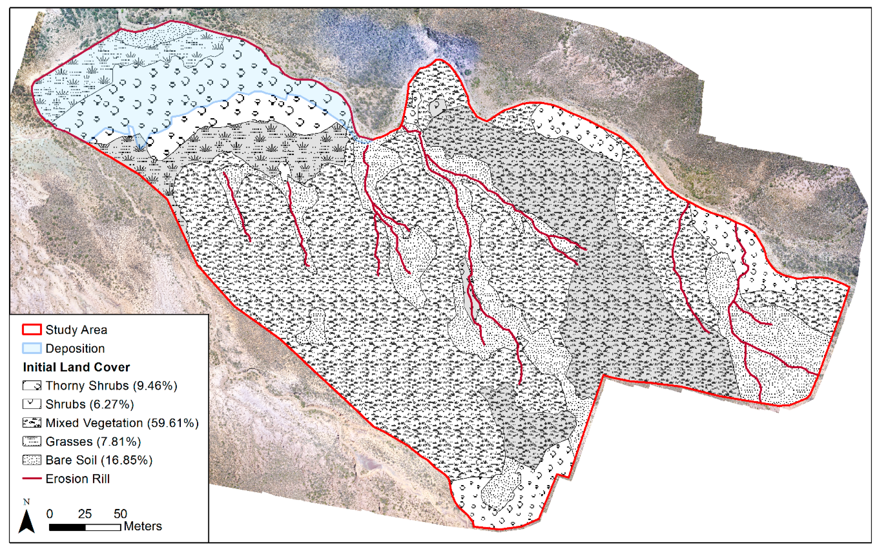
3.1. Field Mapping
3.2. Land Cover Classification and Accuracy
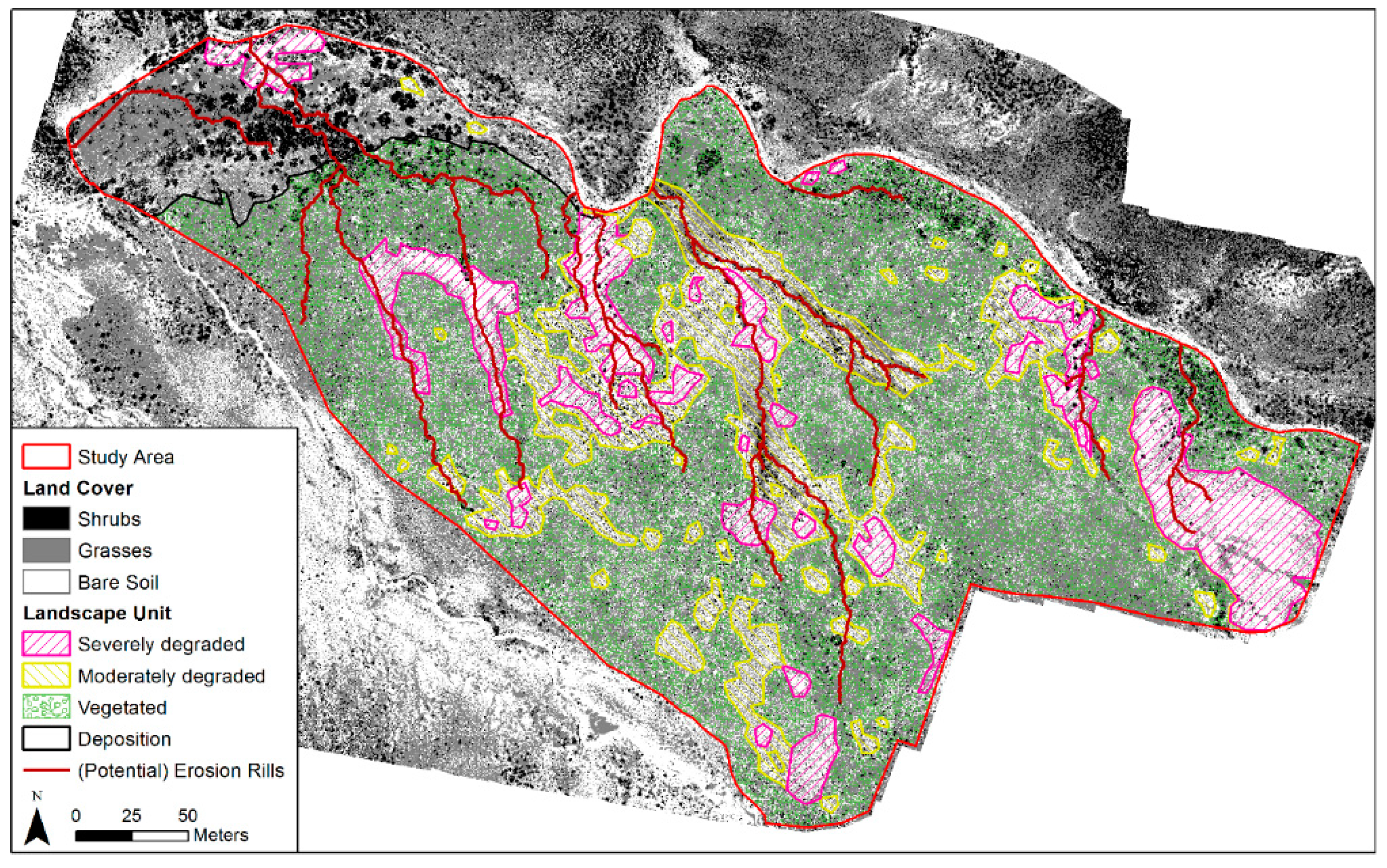
3.3. Mapping Landscape Units
4. Discussion
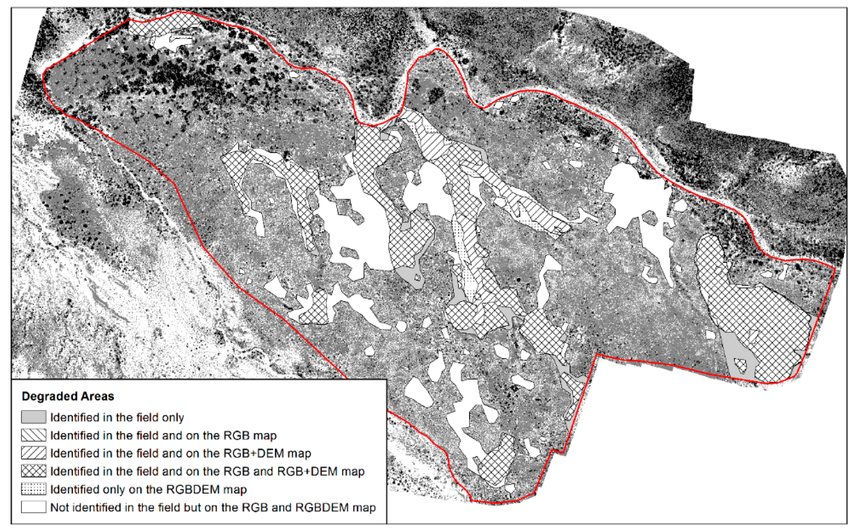
4.1. Comparison of Field Mapping and RGB Map
4.2. Comparison of Field Mapping and RGB+DEM Map
4.3. Comparison of RGB and RGB+DEM Map
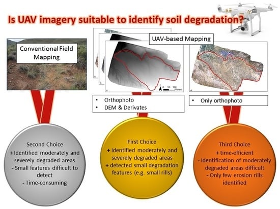
4.4. Potential and Limitations of Using UAV Imagery for Assessing Soil Degradation
4.5. Can Field Mapping Deliver the Status Quo?
5. Conclusions
Author Contributions
Funding
Acknowledgments
Conflicts of Interest
References
- Deblauwe, V.; Barbier, N.; Couteron, P.; Lejeune, O.; Bogaert, J. The global biogeography of semi-arid periodic vegetation patterns. Glob. Ecol. Biogeogr. 2008, 17, 715–723. [Google Scholar] [CrossRef]
- Dickie, J.A.; Parsons, A.J. Eco-geomorphological processes within grasslands, shrublands and badlans in the semi-arid Karro, South Africa. Land Degrad. Dev. 2012, 23, 534–547. [Google Scholar] [CrossRef]
- Dunkerley, D.L.; Brown, K.J. Banded vegetation near Broken Hill, Australia: Significance of surface roughness and soil physical properties. Catena 1999, 37, 75–88. [Google Scholar] [CrossRef]
- Maestre, F.T.; Cortina, J. Spatial patterns of surface soil properties and vegetation in a Mediterranean semi-arid steppe. Plant Soil 2002, 241, 279–291. [Google Scholar] [CrossRef]
- Saco, P.M.; Willgoose, G.R.; Hancock, G.R. Eco-geomorphology of banded vegetation patterns in arid and semi-arid regions. Hydrol. Earth Syst. Sci. 2007, 11, 1717–1730. [Google Scholar] [CrossRef]
- Valentin, C.; d’Herbès, J.M.; Poesen, J. Soil and water components of banded vegetation patterns. Catena 1999, 37, 1–24. [Google Scholar] [CrossRef]
- Couteron, P.; Lejeune, O. Periodic spotted patterns in semi-arid vegetation explained by a propagation-inhibition model. J. Ecol. 2001, 89, 616–628. [Google Scholar] [CrossRef]
- Schlesinger, W.H.; Raikes, J.A.; Hartley, A.E.; Cross, A.F. On the Spatial Pattern of Soil Nutrients in Desert Ecosystems. Ecology 1996, 77, 364–374. [Google Scholar] [CrossRef]
- Schlesinger, W.H.; Reynolds, J.F.; Cunningham, G.L.; Huenneke, L.F.; Jarrell, W.M.; Virginia, R.A.; Whitford, W.G. Biological Feedbacks in Global Desertification. Science 1990, 247, 1043–1048. [Google Scholar] [CrossRef]
- Cammeraat, L.H.; Imeson, A.C. The evolution and significance of soil–vegetation patterns following land abandonment and fire in Spain. Catena 1999, 37, 107–127. [Google Scholar] [CrossRef]
- Bochet, E.; Poesen, J.; Rubio, J.L. Mound development as an interaction of individual plants with soil, water erosion and sedimentation processes on slopes. Earth Surf. Process. Landf. 2000, 25, 847–867. [Google Scholar] [CrossRef]
- Cerdá, A. The effect of patchy distribution of Stipa tenacissima L. on runoff and erosion. J. Arid Environ. 1997, 36, 37–51. [Google Scholar] [CrossRef]
- Rietkerk, M.; Ketner, P.; Burger, J.; Hoorens, B.; Olff, H. Multiscale soil and vegetation patchiness along a gradient of herbivore impact in a semi-arid grazing system in West Africa. Plant Ecol. 2000, 148, 207–224. [Google Scholar] [CrossRef]
- Castillo, V.M.; Martinez-Mena, M.; Albaladejo, J. Runoff and Soil Loss Response to Vegetation Removal in a Semiarid Environment. Soil Sci. Soc. Am. J. 1997, 61, 1116–1121. [Google Scholar] [CrossRef]
- Wynn, T.; Mostaghimi, S. The Effects of Vegetation and Soil Type on Streambank Erosion, Southwestern Virginia, Usa1. JAWRA J. Am. Water Resour. Assoc. 2006, 42, 69–82. [Google Scholar] [CrossRef]
- HilleRisLambers, R.; Rietkerk, M.; van den Bosch, F.; Prins, H.H.T.; de Kroon, H. Vegetation Pattern Formation in Semi-Arid Grazing Systems. Ecology 2001, 82, 50–61. [Google Scholar] [CrossRef]
- Rietkerk, M.; Boerlijst, M.C.; van Langevelde, F.; HilleRisLambers, R.; van de Koppel, J.; Kumar, L.; Prins, H.H.T.; de Roos, A.M. Self-Organization of Vegetation in Arid Ecosystems. Am. Nat. 2002, 160, 524–530. [Google Scholar]
- FAO; ISRIC. UNEP Soil and Terrain Database for Southern Africa, 1:2 M scale. FAO, Rome. Available online: https://www.isric.org/projects/soil-and-terrain-soter-database-programme (accessed on 15 February 2019).
- Dewitte, O.; Jones, A.; Spaargaren, O.; Breuning-Madsen, H.; Brossard, M.; Dampha, A.; Deckers, J.; Gallali, T.; Hallett, S.; Jones, R.; et al. Harmonisation of the soil map of Africa at the continental scale. Geoderma 2013, 211–212, 138–153. [Google Scholar] [CrossRef]
- Hengl, T.; Heuvelink, G.B.M.; Kempen, B.; Leenaars, J.G.B.; Walsh, M.G.; Shepherd, K.D.; Sila, A.; MacMillan, R.A.; de Mendes Jesus, J.; Tamene, L.; et al. Mapping Soil Properties of Africa at 250 m Resolution: Random Forests Significantly Improve Current Predictions. PLoS ONE 2015, 10, e0125814. [Google Scholar] [CrossRef]
- Paterson, G.; Turner, D.; Wiese, L.; van Zijl, G.; Clarke, C.; van Tol, J. Spatial soil information in South Africa: Situational analysis, limitations and challenges. South Afr. J. Sci. 2015, 111. [Google Scholar] [CrossRef]
- Boardman, J.; Foster, I.D.L.; Rowntree, K.M.; Favis-Mortlock, D.T.; Mol, L.; Suich, H.; Gaynor, D. Long-term studies of land degradation in the Sneeuberg uplands, eastern Karoo, South Africa: A synthesis. Geomorphology 2017, 285, 106–120. [Google Scholar] [CrossRef]
- Behrens, T.; Förster, H.; Scholten, T.; Steinrücken, U.; Spies, E.-D.; Goldschmitt, M. Digital soil mapping using artificial neural networks. J. Plant Nutr. Soil Sci. 2005, 168, 21–33. [Google Scholar] [CrossRef]
- Sanchez, P.A.; Ahamed, S.; Carré, F.; Hartemink, A.E.; Hempel, J.; Huising, J.; Lagacherie, P.; McBratney, A.B.; McKenzie, N.J.; de Mendonça-Santos, M.L.; et al. Digital Soil Map of the World. Science 2009, 325, 680–681. [Google Scholar] [CrossRef]
- Nussbaum, M.; Ettlin, L.; Çöltekin, A.; Suter, B.; Egli, M. The relevance of scale in soil maps. Bull. BGS 2011, 32, 63–70. [Google Scholar]
- Behrens, T.; Zhu, A.-X.; Schmidt, K.; Scholten, T. Multi-scale digital terrain analysis and feature selection for digital soil mapping. Geoderma 2010, 155, 175–185. [Google Scholar] [CrossRef]
- Illés, G.; Kovács, G.; Heil, B. Comparing and evaluating digital soil mapping methods in a Hungarian forest reserve. Can. J. Soil Sci. 2011, 91, 615–626. [Google Scholar] [CrossRef]
- Hengl, T. A Practical Guide to Geostatistical Mapping, 2nd ed.; Office for Official Publications of the European Communities: Amsterdam, The Netherlands, 2009; ISBN 978-90-90-24981-0. [Google Scholar]
- Dube, T.; Mutanga, O.; Sibanda, M.; Seutloali, K.; Shoko, C. Use of Landsat series data to analyse the spatial and temporal variations of land degradation in a dispersive soil environment: A case of King Sabata Dalindyebo local municipality in the Eastern Cape Province, South Africa. Phys. Chem. Earth Parts ABC 2017, 100, 112–120. [Google Scholar] [CrossRef]
- Broxton, P.D.; Zeng, X.; Sulla-Menashe, D.; Troch, P.A. A Global Land Cover Climatology Using MODIS Data. J. Appl. Meteorol. Climatol. 2014, 53, 1593–1605. [Google Scholar] [CrossRef]
- Jones, A.; Breuning-Madsen, H.; Brossard, M.; Dampha, A.; Deckers, J.; Dewitte, O.; Gallali, T.; Hallett, S.; Jones, R.; Kilasara, M.; et al. (Eds.) Soil Atlas of Africa; European Commission: Luxembourg, 2013; ISBN 978-92-79-26715-4. [Google Scholar]
- Wang, R.; Zhang, S.; Pu, L.; Yang, J.; Yang, C.; Chen, J.; Guan, C.; Wang, Q.; Chen, D.; Fu, B.; et al. Gully Erosion Mapping and Monitoring at Multiple Scales Based on Multi-Source Remote Sensing Data of the Sancha River Catchment, Northeast China. ISPRS Int. J. Geo-Inf. 2016, 5, 200. [Google Scholar] [CrossRef]
- D’Oleire-Oltmanns, S.; Marzolff, I.; Peter, K.; Ries, J. Unmanned Aerial Vehicle (UAV) for Monitoring Soil Erosion in Morocco. Remote Sens. 2012, 4, 3390–3416. [Google Scholar] [CrossRef]
- Neugirg, F.; Stark, M.; Kaiser, A.; Vlacilova, M.; Della Seta, M.; Vergari, F.; Schmidt, J.; Becht, M.; Haas, F. Erosion processes in calanchi in the Upper Orcia Valley, Southern Tuscany, Italy based on multitemporal high-resolution terrestrial LiDAR and UAV surveys. Geomorphology 2016, 269, 8–22. [Google Scholar] [CrossRef]
- Nobajas, A.; Waller, R.I.; Robinson, Z.P.; Sangonzalo, R. Too much of a good thing? The role of detailed UAV imagery in characterizing large-scale badland drainage characteristics in South-Eastern Spain. Int. J. Remote Sens. 2017, 38, 2844–2860. [Google Scholar] [CrossRef]
- Lucieer, A.; de Jong, S.M.; Turner, D. Mapping landslide displacements using Structure from Motion (SfM) and image correlation of multi-temporal UAV photography. Prog. Phys. Geogr. Earth Environ. 2014, 38, 97–116. [Google Scholar] [CrossRef]
- Nakano, T.; Kamiya, I.; Tobita, M.; Iwahashi, J.; Nakajima, H. Landform monitoring in active volcano by UAV and SfM-MVS technique. In Proceedings of the ISPRS—International Archives of the Photogrammetry, Remote Sensing and Spatial Information Sciences, Hyderabad, India, 9–12 December 2014; Copernicus GmbH: Göttingen, Germany, 2004; Volume XL–8, pp. 71–75. [Google Scholar]
- Bartley, R.; Roth, C.H.; Ludwig, J.; McJannet, D.; Liedloff, A.; Corfield, J.; Hawdon, A.; Abbott, B. Runoff and erosion from Australia’s tropical semi-arid rangelands: Influence of ground cover for differing space and time scales. Hydrol. Process. 2006, 20, 3317–3333. [Google Scholar] [CrossRef]
- Ludwig, J.A.; Bastin, G.N.; Chewings, V.H.; Eager, R.W.; Liedloff, A.C. Leakiness: A new index for monitoring the health of arid and semiarid landscapes using remotely sensed vegetation cover and elevation data. Ecol. Indic. 2007, 7, 442–454. [Google Scholar] [CrossRef]
- Puigdefábregas, J. The role of vegetation patterns in structuring runoff and sediment fluxes in drylands: Vegetation and sediment fluxes. Earth Surf. Process. Landf. 2005, 30, 133–147. [Google Scholar] [CrossRef]
- Rogers, R.D.; Schumm, S.A. The effect of sparse vegetative cover on erosion and sediment yield. J. Hydrol. 1991, 123, 19–24. [Google Scholar] [CrossRef]
- Esler, K.J.; Milton, S.J.; Dean, W.R.J. (Eds.) Karoo Veld Ecology and Management, 1st ed.; Briza: Pretoria, South Africa, 2006; ISBN 978-1-875093-52-6. [Google Scholar]
- Foster, I.D.L.; Boardman, J.; Keay-Bright, J.; Meadows, M.E. Land degradation and sediment dynamics in the South African Karoo. In Sediment Budgets 2, Proceedings of the Symposium S1 Held during the Seventh IAHS Scientific Assembly at Foz do Iguaçu, Brazil, 3–9 April 2005; Horowitz, A.J., Walling, D.E., Eds.; IAHS Publication; Int Assoc Hydrological Sciences: Wallingford, CT, USA, 2005; pp. 207–213. ISBN 978-1-901502-92-3. [Google Scholar]
- Keay-Bright, J.; Boardman, J. The influence of land management on soil erosion in the sneeuberg mountains, central Karoo, south Africa. Land Degrad. Dev. 2007, 18, 423–439. [Google Scholar] [CrossRef]
- Mighall, T.M.; Foster, I.D.L.; Rowntree, K.M.; Boardman, J. Reconstructing recent land degradation in the semi-arid Karoo of South Africa: A palaeoecological study at Compassberg, Eastern Cape. Land Degrad. Dev. 2012. [Google Scholar] [CrossRef]
- Boardman, J.; Foster, I.D. The potential significance of the breaching of small farm dams in the Sneeuberg region, South Africa. J. Soils Sediments 2011, 11, 1456–1465. [Google Scholar] [CrossRef]
- Krenz, J.; Kuhn, N.J. Assessing Badland Sediment Sources Using Unmanned Aerial Vehicles. In Badlands Dynamics in a Context of Global Change; Elsevier: Amsterdam, The Netherlands, 2018; pp. 255–276. ISBN 978-0-12-813054-4. [Google Scholar]
- Huang, C.; Davis, L.S.; Townshend, J.R.G. An assessment of support vector machines for land cover classification. Int. J. Remote Sens. 2002, 23, 725–749. [Google Scholar] [CrossRef]
- Mondal, A.; Kundu, S.; Chandniha, S.K.; Shukla, R.; Mishra, P.K. Comparison of support vector machine and maximum likelihood classification technique using satellite imagery. Int. J. Remote Sens. GIS 2012, 1, 116–123. [Google Scholar]
- Szuster, B.W.; Chen, Q.; Borger, M. A comparison of classification techniques to support land cover and land use analysis in tropical coastal zones. Appl. Geogr. 2011, 31, 525–532. [Google Scholar] [CrossRef]
- Foody, G.M.; Mathur, A. A relative evaluation of multiclass image classification by support vector machines. IEEE Trans. Geosci. Remote Sens. 2004, 42, 1335–1343. [Google Scholar] [CrossRef]
- Thompson, M. A standard land-cover classification scheme for remote-sensing applications in South Africa. South Afr. J. Sci. 1996, 92, 34–42. [Google Scholar]
- Congalton, R.G. Accuracy assessment and validation of remotely sensed and other spatial information. Int. J. Wildland Fire 2001, 10, 321–328. [Google Scholar] [CrossRef]
- Jensen, J.R. Introductory Digital Image Processing: A Remote Sensing Perspective, 2nd ed.; Prentice Hall series in geographic information science; Prentice Hall: Upper Saddle River, NJ, USA, 1996; ISBN 978-0-13-205840-7. [Google Scholar]
- Morgan, R.P.C. Soil Erosion and Conservation, 3rd ed.; Blackwell Publishing: Malden, MA, USA, 2005; ISBN 978-1-4051-1781-4. [Google Scholar]
- Jenny, H. Factors of Soil Formation: A System of Quantitative Pedology; Cole, L.J., Ed.; McGraw Hill: New York, NY, USA, 1941; ISBN 0-486-68128-9. [Google Scholar]
- Moore, I.D.; Gessler, P.E.; Nielsen, G.A.; Peterson, G.A. Soil Attribute Prediction Using Terrain Analysis. Soil Sci. Soc. Am. J. 1993, 57, 443–452. [Google Scholar] [CrossRef]
- Dobos, E.; Hengl, T. Chapter 20 Soil Mapping Applications. In Developments in Soil Science; Hengl, T., Reuter, H.I., Eds.; Geomorphometry; Elsevier: Amsterdam, The Netherlands, 2009; Volume 33, pp. 461–479. [Google Scholar]
- Schwanghart, W.; Groom, G.; Kuhn, N.J.; Heckrath, G. Flow network derivation from a high resolution DEM in a low relief, agrarian landscape. Earth Surf. Process. Landf. 2013, 38, 1576–1586. [Google Scholar] [CrossRef]
- Schäuble, H.; Marinoni, O.; Hinderer, M. A GIS-based method to calculate flow accumulation by considering dams and their specific operation time. Comput. Geosci. 2008, 34, 635–646. [Google Scholar] [CrossRef]
- Weiss, A. Topographic position and landforms analysis. In Proceedings of the Poster Presentation, ESRI User Conference, San Diego, CA, USA, 9–13 July 2001; Volume 200. [Google Scholar]
- Römkens, M.J.; Helming, K.; Prasad, S.N. Soil erosion under different rainfall intensities, surface roughness, and soil water regimes. Catena 2002, 46, 103–123. [Google Scholar] [CrossRef]
- Smith, J.H.; Stehman, S.V.; Wickham, J.D.; Yang, L. Effects of landscape characteristics on land-cover class accuracy. Remote Sens. Environ. 2003, 84, 342–349. [Google Scholar] [CrossRef]
- Bannari, A.; Morin, D.; Bonn, F.; Huete, A.R. A review of vegetation indices. Remote Sens. Rev. 1995, 13, 95–120. [Google Scholar] [CrossRef]
- Geerken, R.; Zaitchik, B.; Evans, J.P. Classifying rangeland vegetation type and coverage from NDVI time series using Fourier Filtered Cycle Similarity. Int. J. Remote Sens. 2005, 26, 5535–5554. [Google Scholar] [CrossRef]
- Su, L.; Chopping, M.J.; Rango, A.; Martonchik, J.V.; Peters, D.P.C. Support vector machines for recognition of semi-arid vegetation types using MISR multi-angle imagery. Remote Sens. Environ. 2007, 107, 299–311. [Google Scholar] [CrossRef]
- Xie, Y.; Sha, Z.; Yu, M. Remote sensing imagery in vegetation mapping: A review. J. Plant Ecol. 2008, 1, 9–23. [Google Scholar] [CrossRef]


| Vegetation Cover | Description | Implication | Land Cover (LC) | Identification from the Orthophoto | |
|---|---|---|---|---|---|
| Bare soil | Areas (>1 m2) of exposed sand, soil, or rock with no or very little vegetation | Threatened by erosion due to lack of protecting vegetation cover |  | Bare Soil | Higher overall reflectance (whiter appearance) → areas of mostly white to sandy colors (often slightly yellow or orange) with no apparent line structure that could indicate grasses; stones often very white and characterized through their angular shape |
| Rills | Rill structure of bare soil, no or little shrub vegetation | Threatened by intensive erosion due to concentrated runoff | |||
| Woody-plants dominating, typically broad-leaved, branching at or near the ground, up to 1 m in height | Threatened by erosion if roots are exposed or shrubs grow on pedestals |  | Shrubs | In this area characterized by a light bright green to dark green or blueish green color | |
| Thorny Shrubs | Woody-plants with thorns dominating, up to 1 m in height, mostly Lycium horridum | Threatened by erosion if roots are exposed or shrubs grow on pedestals | |||
| Mixed Vegetation | Areas where neither grasses nor shrubs are dominant | Threatened by erosion if vegetation cover <50% | |||
| Grasses | Non-woody, grass-like, herbaceous plants dominating, grass-like plants often grow as tussocks | Threatened by erosion if vegetation cover <50% or tussock grasses grow on pedestals |  | Grasses | Color appearance is more faded (beige to light grey green) than the color of the shrubs; in a high resolution image grasses can be distinguished from shrubs by their long, narrow, and sometimes curled leaves |
| Reference Data | ||||||
|---|---|---|---|---|---|---|
| LC Class | Shrubs | Grasses | Bare Soil | Total | User’s Accuracy | |
| Classified Data | Shrubs | 111 | 37 | 2 | 150 | 74% |
| Grasses | 20 | 114 | 16 | 150 | 76% | |
| Bare Soil | 2 | 21 | 127 | 150 | 85% | |
| Total | 133 | 172 | 145 | 450 | ||
| Producer’s Accuracy | 83% | 66% | 88% | 78% | ||
| Kappa | 0.67 | |||||
| Landscape Unit (LU) | Identification | Area (ha) | ||
|---|---|---|---|---|
| In Field | On UAV Imagery/DEM/Derivative | RGB Map | RGB+DEM Map | |
| Depositional | Flat terrain behind the former dam wall | Former reservoir area on historical aerial images, sharp elevation change at the dam wall | 1.02 | 1.02 |
| Severely degraded | Crusted soils | 0.72 | 1.23 | |
| Contiguous area of bare soil with little vegetation (individual shrubs or tussock grass) and large gaps between individual plants, vegetation cover <30% | ||||
| Clearly developed rills | ||||
| Moderately degraded | Very low TPI | 1.6 | 1.55 | |
| Contiguous area of bare soil more regularly interspersed with vegetation but vegetation cover <50% | ||||
| Some rills | ||||
| Erosion rill | Rill structure | Line structure of bare soil, possibly flow accumulation paths on DEM | 0.95 * | 2.12 * |
| Very low TPI | ||||
| Vegetated | Contiguous vegetation cover interspersed with patches of bare soil or stones, at least 50% covered with vegetation | 6.47 | 6.15 | |
© 2019 by the authors. Licensee MDPI, Basel, Switzerland. This article is an open access article distributed under the terms and conditions of the Creative Commons Attribution (CC BY) license (http://creativecommons.org/licenses/by/4.0/).
Share and Cite
Krenz, J.; Greenwood, P.; Kuhn, N.J. Soil Degradation Mapping in Drylands Using Unmanned Aerial Vehicle (UAV) Data. Soil Syst. 2019, 3, 33. https://doi.org/10.3390/soilsystems3020033
Krenz J, Greenwood P, Kuhn NJ. Soil Degradation Mapping in Drylands Using Unmanned Aerial Vehicle (UAV) Data. Soil Systems. 2019; 3(2):33. https://doi.org/10.3390/soilsystems3020033
Chicago/Turabian StyleKrenz, Juliane, Philip Greenwood, and Nikolaus J. Kuhn. 2019. "Soil Degradation Mapping in Drylands Using Unmanned Aerial Vehicle (UAV) Data" Soil Systems 3, no. 2: 33. https://doi.org/10.3390/soilsystems3020033