Vibration Measurements by Self-Mixing Interferometry: An Overview of Configurations and Benchmark Performances

Abstract

Self-mixing interferometry (SMI) is suitable to sense and measure vibrations of amplitudes ranging from picometers to millimeters at frequencies from sub-Hz to MHz’s. As an optical probe, SMI has the advantage of being non-invasive with the ability to measure without any treatment of the target surface and operate from a substantial standoff distance from the target. As an additional advantage, the SMI configuration is much simpler than that of conventional interferometers as it does not require any optical part external to the laser source. After a short introduction to the basics of SMI, we review the development of configurations of SMI instruments for vibration measurements, based on both analog and digital processing, with record performance to cover the range of vibration amplitudes from 0.1 nm to 1 mm, frequencies up to MHz, and stand-off distances up to 100 m. These performances set a benchmark that is unequaled by other approaches reported so far in the literature. The configurations we describe are (i) a simple MEMS-response testing instrument based on fringe counting, (ii) a half-fringe locking vibrometer for mechanical mode analysis and transfer function measurements, with a wide linear response on six decades of amplitude, (iii) a vibrometer with analog switching cancellation for μm-to-mm amplitude of vibrations, and (iv) a long standoff distance vibrometer for testing large structures at distances up to 100 m and with nm sensitivity. Lastly, as the vibrometer will almost invariably operate on untreated, diffusing surfaces, we provide an evaluation of phase-induced speckle pattern errors affecting the SMI measurement.

1. Introduction

Optical techniques are attractive for vibration measurements because they are non-invasive, fast, and accurate [1,2]. A straightforward optical technique like triangulation [3] supplies an appreciable sensitivity in the measurement of small vibrations—for example, resolving 15 μm for a parallax resolution of Δα = 0.3 mr and a base D and standoff distance L both of 5 cm [3,4]. However, coherent techniques like interferometry outperform this result of decades, offering sub-nm resolution, a dynamic range up to mm, standoff distances up to hundreds of meters, MHz bandwidth, and, last but not least, a compact and inexpensive setup.

In this introduction, we briefly recall the principle of laser interferometry and the most recent version of it, self-mixing interferometry (SMI). Among the several applications of SMI that have been demonstrated, in this paper, we focus exclusively on the measurement of vibrations, that is, periodic (and most frequently) sinusoidal small movement of the target. We will not treat other self-mixing measurements or applications like, for example, displacement [5,6,7,8], distance [9,10], velocity and flow rate [11,12], planarity [3], angle [13,14,15], physical quantities (thickness and index of refraction [16,17], linewidth [18], and alpha-factor [19]), the use of self-mix as a detector of optical echoes [20,21], or consumer applications like scroll [22] and gesture AR/VR [23] sensors. The interested reader may also consult general reviews [24] and tutorials like those provided by Refs. [25,26].

1.1. The Laser Interferometer

The first experiments using interferometry date back to 150 years ago. However, only with the advent of the laser, and thanks to its exceptional coherence, has it been exploited in a number of scientific and industrial applications.

As interferometry uses the interference of superposed beams and generates a signal modulated with the wavelength period, its resolution allows the measurement of very minute displacements down to a small fraction of wavelength.

The concept was implemented into a very successful industrial product called the “Laser Interferometer” (LI), the famous HP5525 model introduced in 1967 by Hewlett Packard for the calibration of machine tools, an instrument is capable of resolving displacements in steps of λ/8 = 79 nm with a counting speed of 5 MHz on a distance range of a few meters [3,27].

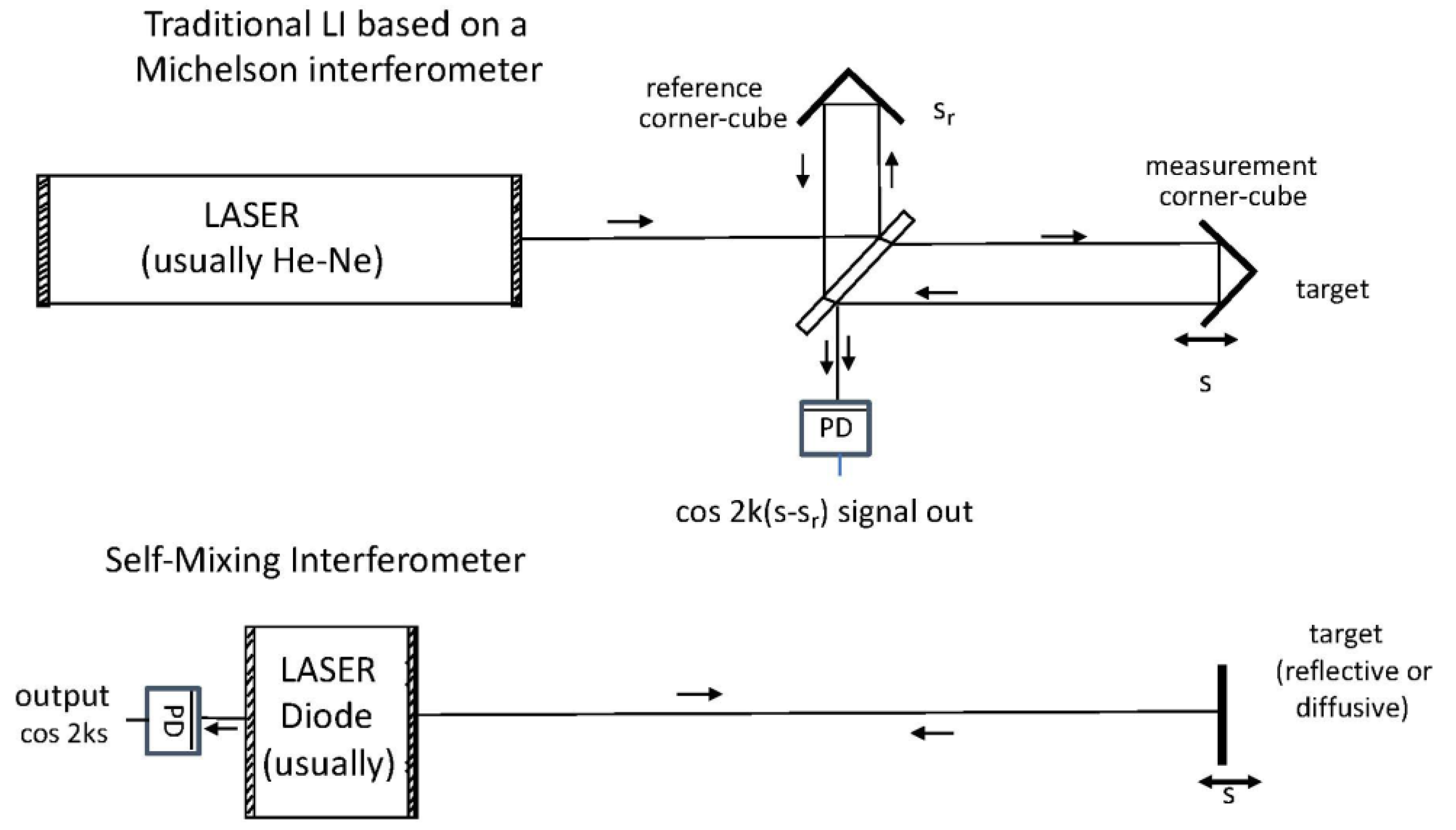
Following a number of variants from several manufacturers, like the one reported in Figure 1 (top), the LI was then basically made around a λ-stabilized He-Ne laser and an external optical interferometer—typically, a Fabry–Perot configuration. The two beams propagated to the target being measured at distance s and to the fixed reference path s_r were superposed at a detector, generating a signal I = I₀ cos 2k(s − s_r), where k = 2π/λ is the wavenumber [28].

Counting the zero-crossing of signal I, variations Δs of a quarter wavelength could be easily measured. Eventually, after adding a second signal I* = I₀ sin 2k(s_m − s_r) obtained with polarization splitting of the interferometer [28], the number of zero-crossings was doubled, thus bringing the resolution to λ/8, which is the performance available in commercial products.

It is worth noting that the LI works in the digital mode, with up/down counting of λ/8 displacement variations Δs_m and requires a corner cube as the target for operation. The corner cube ensures the angular alignment of reference and measurement beams, relieving the user from painstaking alignment operations, and, importantly, it prevents retroreflection from the target (which is seen to disturb its λ-stabilization) from entering the laser cavity. When the retroreflection process is well controlled, we obtain the self-mixing interferometer (SMI) configuration shown in Figure 1 (bottom), and analyzing this configuration, we find that the perturbed cavity field carries both amplitude (AM) and frequency (FM) modulations in the form of two orthogonal signals, cos 2ks and sin 2ks (at weak feedback). The AM component is detected using the monitor photodiode PD, usually mounted in the laser package by the manufacturer for the purpose of controlling the emitted power.

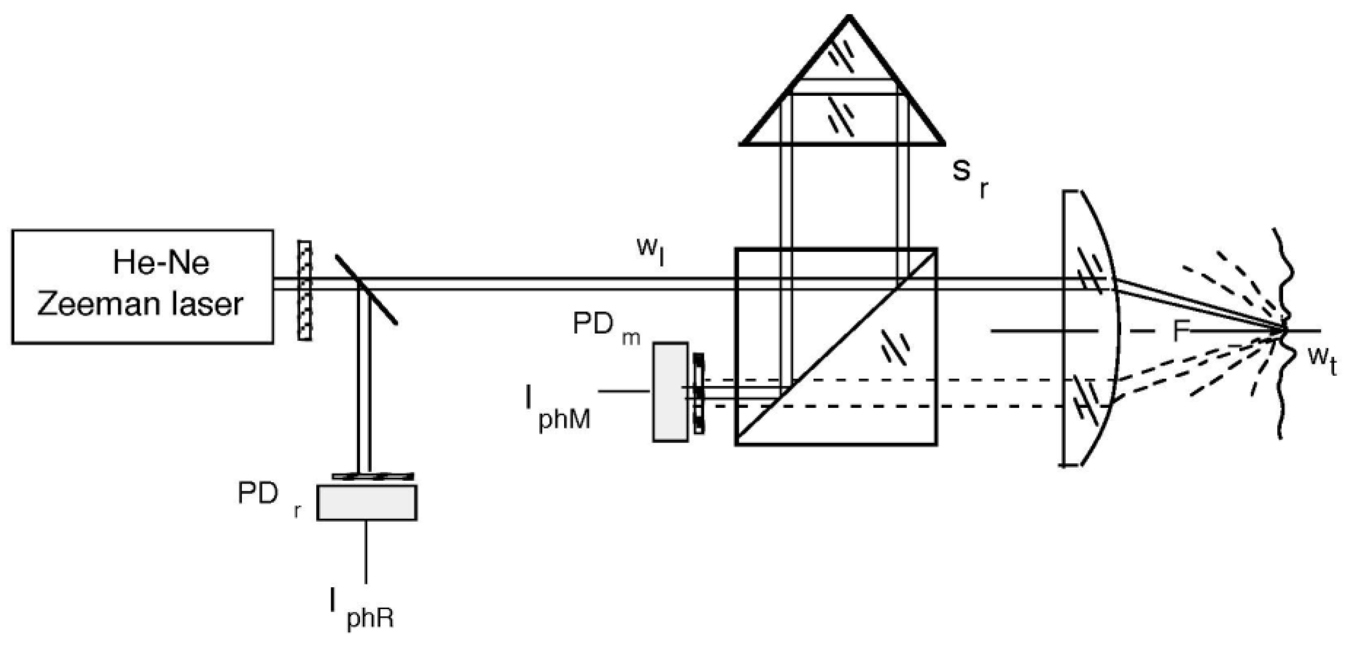
For a vibration measurement, we shall modify the basic configuration of the SMI with a lens in place of the measurement corner cube, as shown in Figure 2, to allow the incoming and outgoing beams to be superposed correctly at the beamsplitter. With this modification, we obtain a laser vibrometer that reads the vibration amplitude digitally, in steps of λ/8 (=79 nm for the 633 nm He-Ne laser) and has a dynamic range (or maximum measurable amplitude) limited by a fraction of the lens focal length (and with typical values of 5–20 mm in practice).

It is worth noting that the configuration can work with a considerable stand-off distance (typically, meters) just by increasing the distance of the lens from the beamsplitter.

1.2. The Self-Mixing Interferometer (SMI)

The SMI has several advantages with respect to the LI because (i) it has a minimum part count (no optical interferometer necessary), so it is potentially low-cost; (ii) it is self-aligned, as it takes the measurement where the spot falls; (iii) it requires no filter to remove ambient light, as the laser cavity performs this function; (iv) the vibration signal is available everywhere on the beam and also at the target side; and (v) it has good performance for small signals (close to the quantum limit, typically 10 pm) and bandwidths (up to MHz) and a wide dynamic range (depending on coherence length) [24,25].

On the other hand, the metrological precision of the λ-stabilized LI (typically six decimal places) is not usually required in vibration measurements and prompts the use of a cheap and compact laser diode (that also includes the photodiode), offering a precision of two to three decimal places (three to four in thermally controlled units).

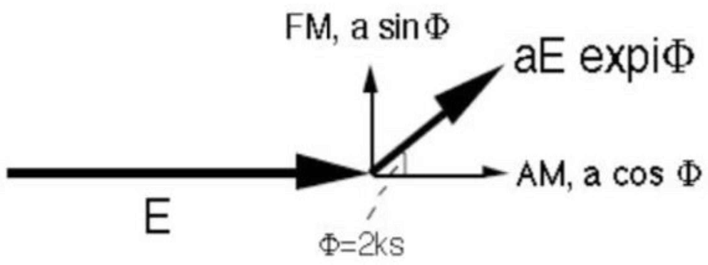
To explain the working principle of the SMI, many approaches have been devised at increasing levels of coverage [24,25]; yet, the simplest one based on rotating-vector modeling (Figure 3) already explains the mechanism of operation. Indeed, we represent the unperturbed cavity field with a rotating vector E (which rotates at the optical frequency) so that the returning rotating field received by the laser cavity is aE exp iϕ, where a is the attenuation and ϕ = 2ks the optical phase shift accumulated along the go-and-return path to the target.

Now, the summation of rotating vectors E and aE exp iϕ, which take place in the cavity, generates amplitude (AM) and frequency (FM) modulations of the resulting field E_R.

The in-phase component of the returning field is aE cos ϕ and produces the increase (decrease) in the resultant field according to the positive (negative) sign of cos ϕ. Thus, an AM of perturbed field is generated, with a modulation index m_AM = a cos ϕ.

Similarly, the in-quadrature component aE sin ϕ either accelerates or decelerates the rotating field according to the sign of sin ϕ. Thus, it is responsible for an FM with a modulation index m_FM = a sin ϕ.

In addition, by considering the time-dependent evolution of the rotating vector addition, it is found that when a is large enough, the trajectory of the resulting field makes a loop—or there is a switching both in amplitude and frequency [24,25].

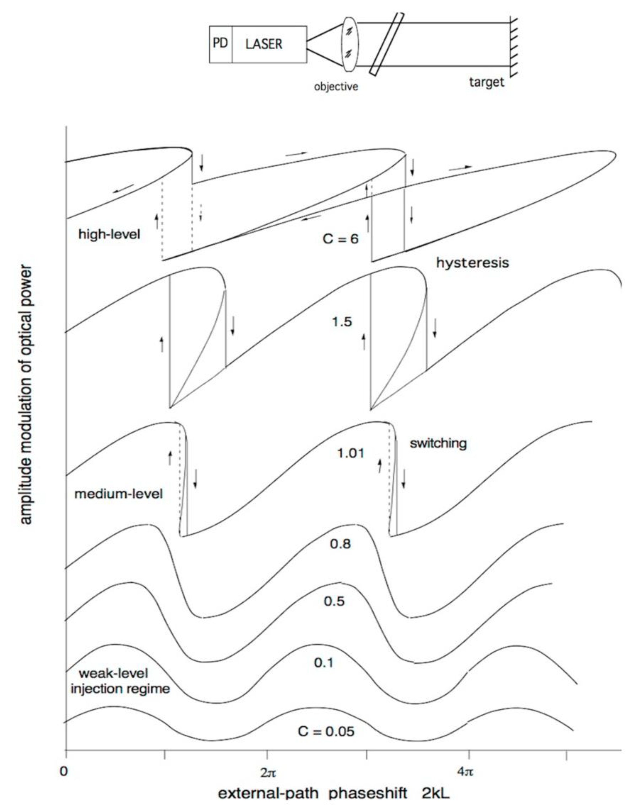
In Figure 4, we can see the evolution of the amplitude waveform E_R. The evolution is governed by the feedback parameter C, which is proportional to the distance times the fraction of returning field [29]. At small C (say, ≤0.05), the waveform of the SMI field E_R is sinusoidal, and the output signal detected by the photodiode PD follows the dependence I = I₀ cos 2ks of a normal interferometer (Figure 4, bottom traces). At increasing feedback, we first notice a distortion in the cosine waveform, with the leading edge becoming slower than the trailing edge (C = 0.1 to 0.8 in Figure 4). Then, we obtain switching from top to bottom at increasing phase shifts (C ≥ 1), which will become a bottom-to-top when phase shift ϕ = 2ks decreases [24,25].

In the experiment, we change the feedback level using a variable attenuator, drive the target with a sine wave, and observe the waveforms exactly as predicted by theory.

It is very important to note that the periodicity of the SMI waveform is always λ/2 at any C, and in each period of the SMI signal, the upgoing switching is for increasing and the down-going switching is for decreasing distance, thus supplying the sign of the λ/2 variations Δs of target distance. This circumstance was used to build a single-channel SMI displacement measuring instrument [8,24] around an 850 nm laser diode, capable of following the displacement of a diffusive target with a digital readout in steps of λ/2 = 425 nm, with a bandpass of 1 MHz (or a target speed up to 0.42 m/s), and a 1 to 2 m distance range.

When the C factor is increased above C = 4.6, we enter a strong regime of feedback, with two switchings per period, at C = 7.85 and above three per period. At still larger values, the switching becomes erratic [30], and the laser exhibits a regime of chaotic oscillations. But, staying at 1 < C < 4.6, the moderate feedback regime, the laser works in a stable and reliable way that is totally suitable for measurements applications.

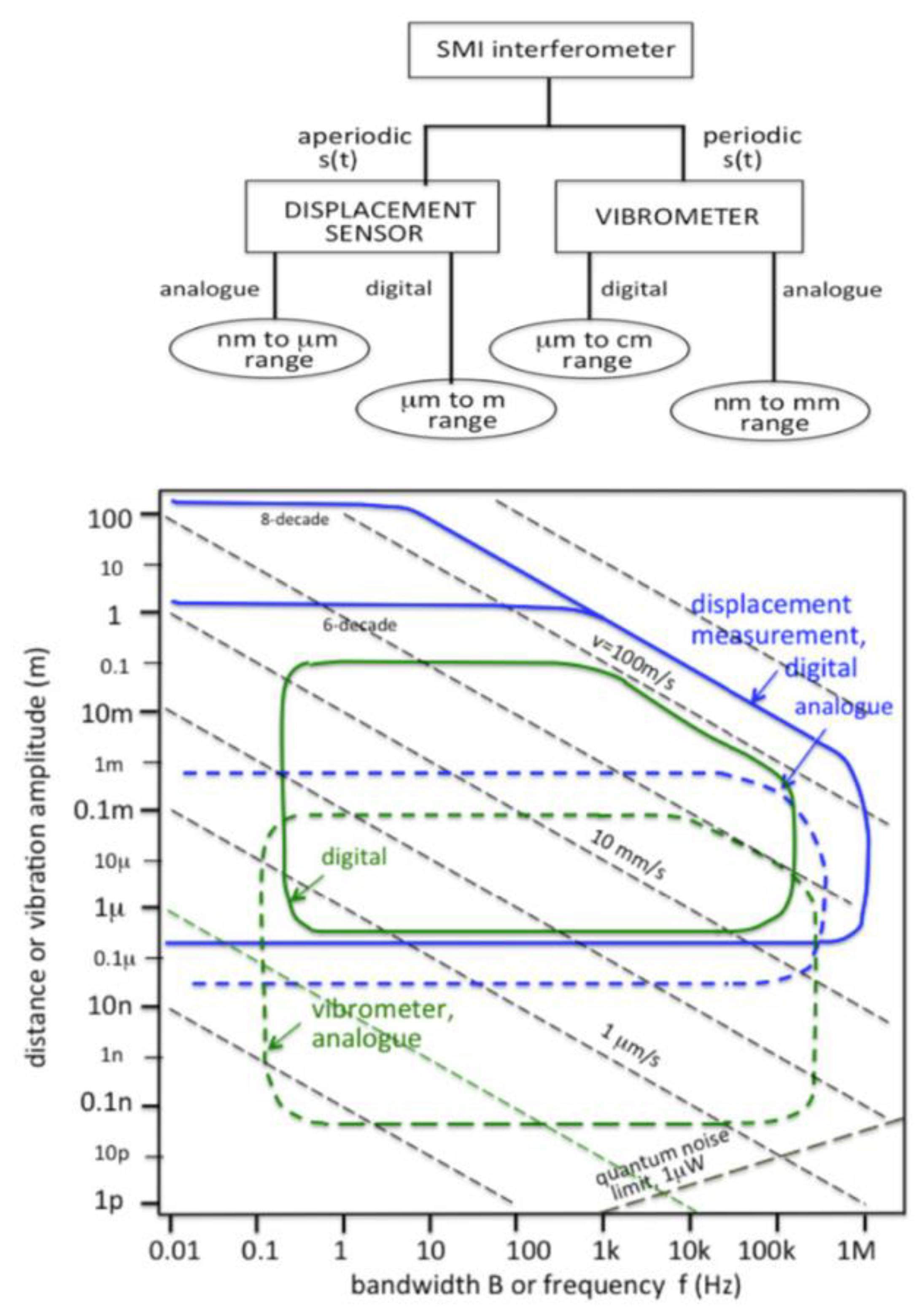
2. Classification of SMI Instruments and Their Typical Performance

From an application point of view, it is fundamental to classify interferometric instruments into two categories, as shown in Figure 5 (top): (i) displacement-measuring instruments, when the s(t) measurand is aperiodic and the time-dependence is arbitrary—this is the case of the machine-tool turret positioning—and (ii) vibration-measuring instrument, when the s(t) waveform is periodic—this is the case of a mechanical transfer response study.

Note that a displacement measurement is incremental, usually based on up/down counting of fringes or fraction thereof, and thus requires an initial zeroing operation. We can also develop (iii) an absolute distance meter, typically using sweeping wavelength [9,10,25] but with lower resolution.

A further classification for interferometric and SMI instruments is according to the type of signal processing used in the instrument, either analog or digital.

The performance of SMI displacement and the vibration SMI instrument with respect to the measurable amplitude and bandwidth of s(t) is summarized in the chart shown in Figure 5 (bottom).

Analog processing is best suited to approach minimum detectable signal set by quantum noise, whereas digital processing has a wider dynamic range of measurement.

For each class of instrument, we find a minimum and maximum measurable signal amplitude as well as a low- and high-frequency cutoff, to which we shall add the Doppler limit due to the target speed v = ds(t)/dt, which increases the bandwidth content of the interferometric signal as v/λ and thus introduces a boundary at −45 degrees, as shown in Figure 5.

Regarding vibrometers, in the following, we review preferred design schematics to implement vibrometers that offer full coverage of the range of performance reported in Figure 5 as well as a range of standoff distances for operation. Then, we briefly discuss the applications for which these vibrometers have been developed.

These case studies represent benchmarks of vibrometer performance that should be borne in mind when developing new solutions because of their proven performance, particularly simple and cheap structure, and minimal requirement for processing the detected signals.

Other than measuring displacements in λ/2 steps, the SMI basic configuration can obviously be used as a vibrometer giving a digital readout with an amplitude resolution of about Δs = λ/2 = 0.4 μm, a dynamic range of counting up to s₀ = 1 m with a counting speed of f₂ = 1 MHz, and coverage of frequency of oscillation given by f₂ Δs/s₀. The digital readout is adequate for measuring vibration amplitudes of say, 50 μm at a frequency f = 10 kHz but suffers from the inverse s₀ dependence of bandwidth at a large dynamic range.

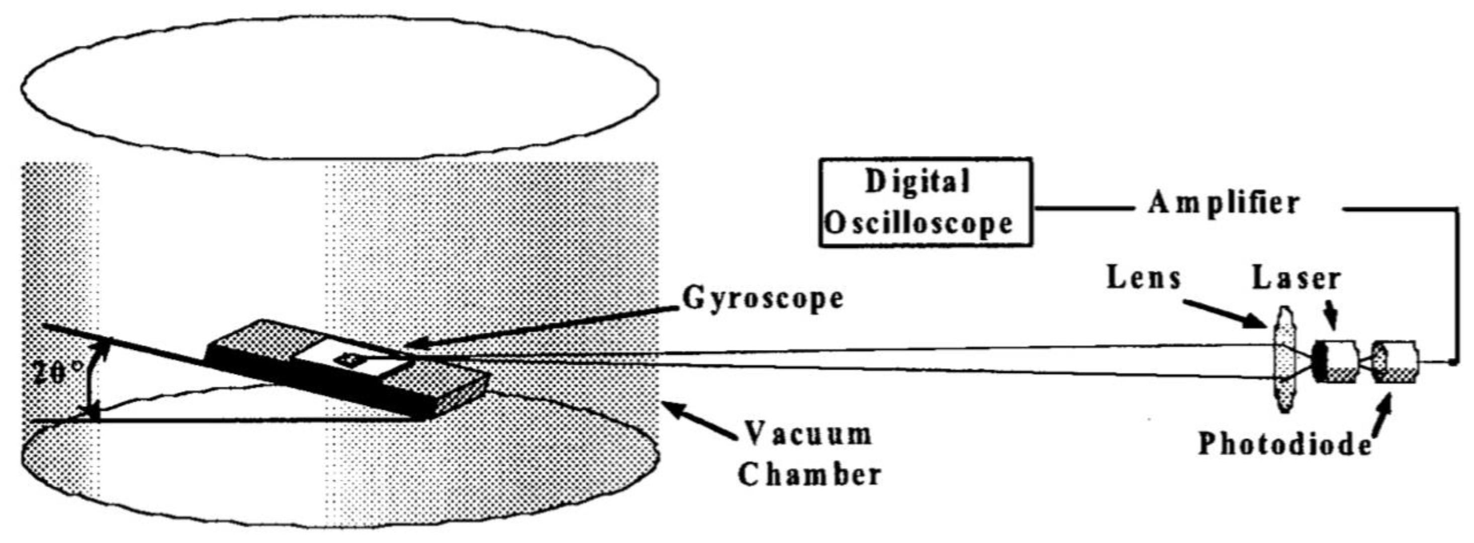
3. Transfer Function Measured Using a Digital Readout (DR) SMI Vibrometer

To illustrate the performance of an SMI interferometer used as a digital readout vibrometer, we now describe its application to the measurement of the mechanical transfer frequency response of a miniature device, a MEMS (micro-electro-mechanical system) [31,32]. The device is a MEMS gyroscope, with a suspended test mass and 2-D comb structure to actuate and read the Coriolis’ force developed by inertial rotation.

As we can see in Figure 6, the SMI is in the basic setup, and we read the signal at the output of the photodiode. A lens focuses the 850 nm laser beam on the 100 × 100 μm² test mass at a slant angle of 20 degrees to develop a measurable component when the mass vibrates in plane. The gyroscope is kept under vacuum to eliminate the damping due to the air. 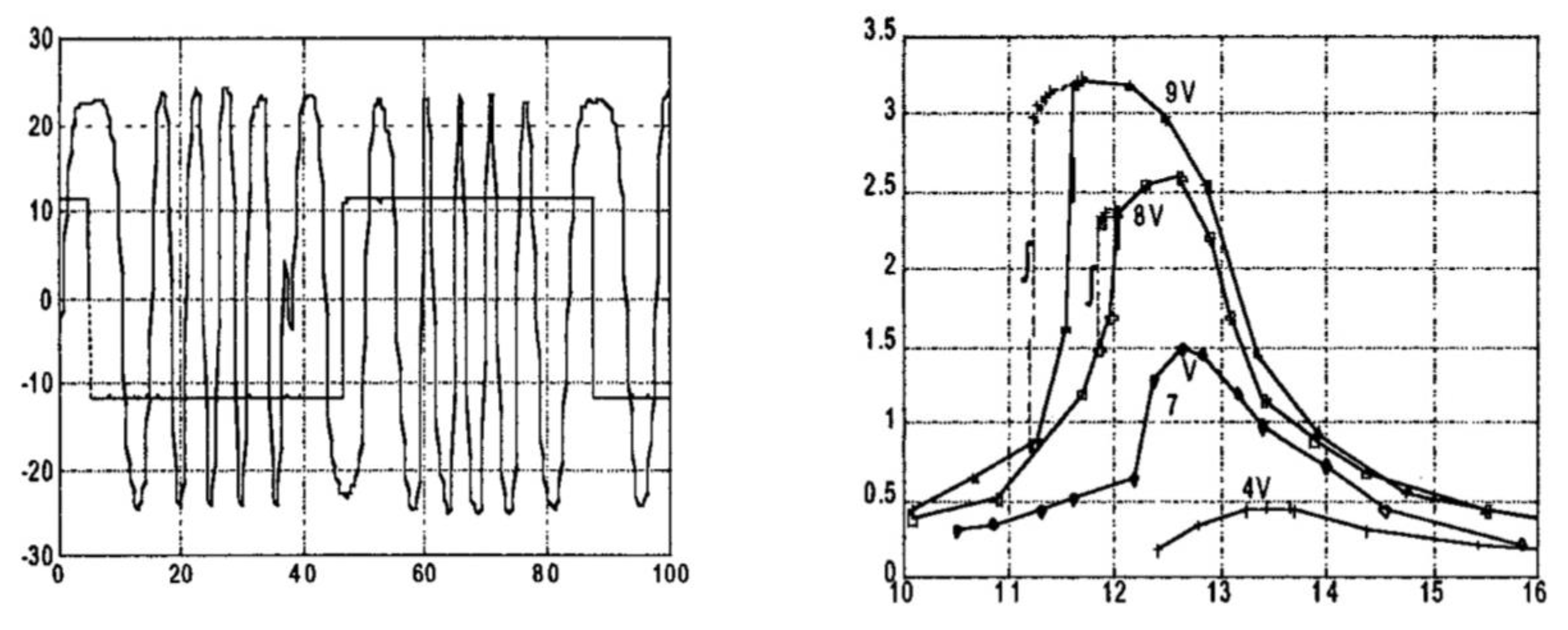By exciting the device with the operating square wave (Figure 7, left), we obtain an SMI signal containing fringes that are easily measured (or even simpler, counted by sight). By repeating the measurement at several excitation frequencies, we can easily build up the frequency response of the MEMS, as shown in Figure 7 on the right.

Several details in Figure 7 are worth noting. First of all, we are able to measure the resonance frequency f_res of the device and its linewidth Δf_res (due to damping). Also, we can measure the dependence of f_res from the drive voltage and find that it decreases with the increasing amplitude of the drive. Last and quite important, performing the measurement at increasing and then decreasing frequency, we may detect a hysteresis of the response curve, which is a premonitory of mechanical creep known to eventually lead to soft failure of the device.

Of course, if we wish to avoid hysteresis, we shall work at a safe drive voltage, as we can read from Figure 7 on the right. Similarly, hysteresis is also found in the response vs. residual air pressure inside the MEMS package. Thus, the SMI in its simplicity is a powerful diagnostic tool for assessing the appropriate working conditions (voltage, pressure, etc.) of the device.

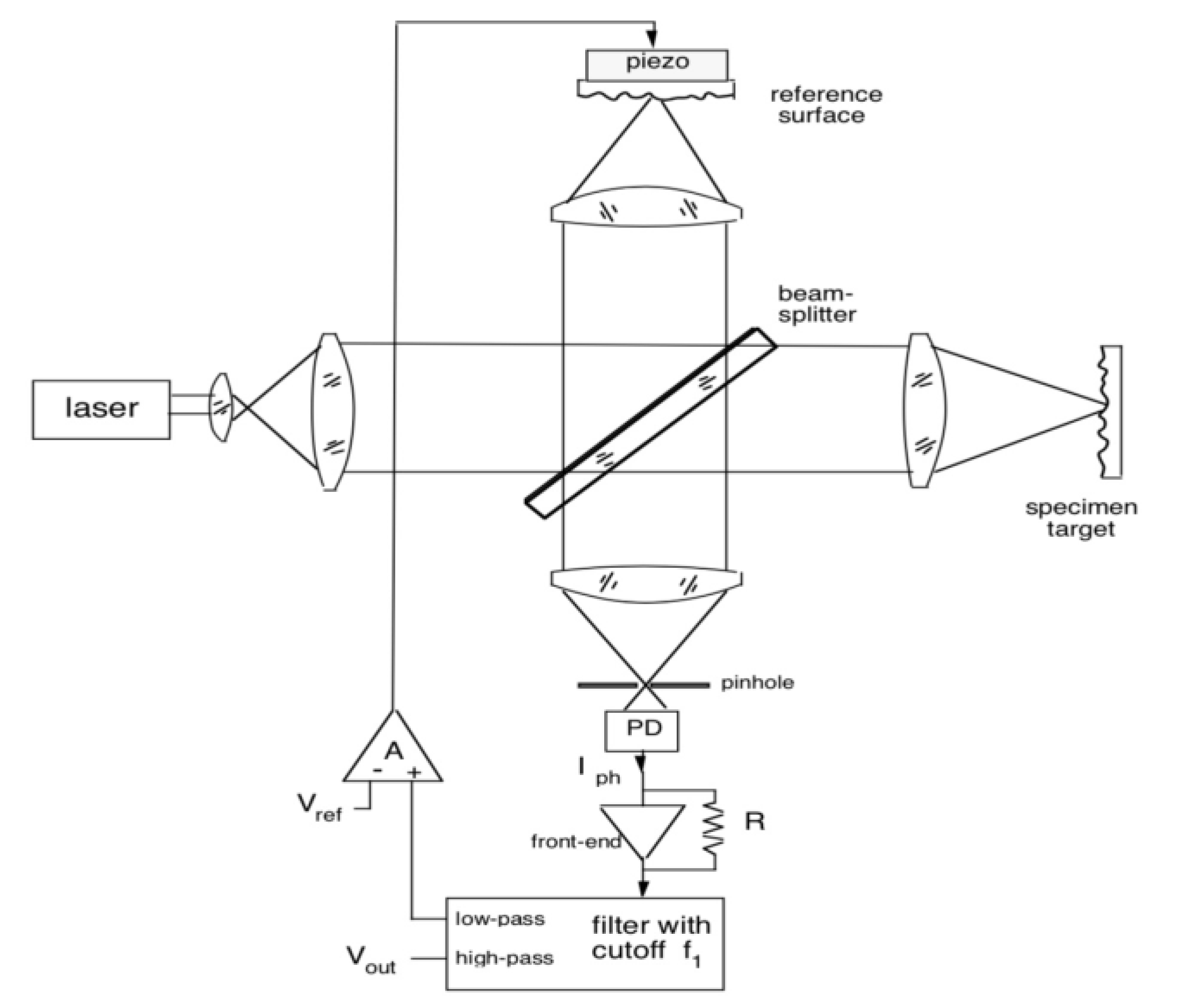
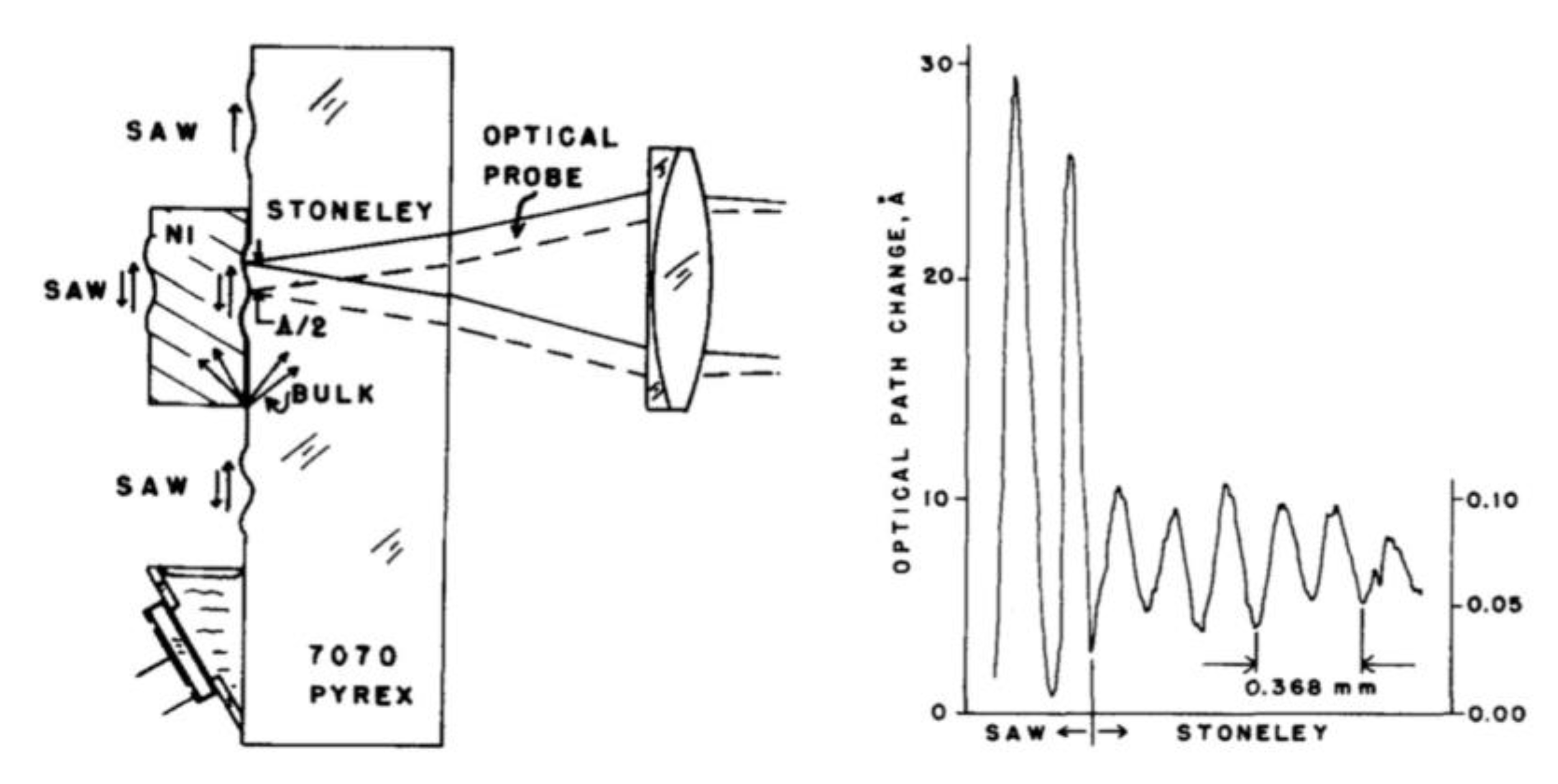
4. Half-Fringe-Stabilized (HFS) Analog Readout SMI Vibrometer

Stabilization of the LI working point at half-fringe is a well-known technique that is useful to read vibrations much smaller than the λ/2 fringe amplitude. The scheme is depicted in Figure 8, where the reference arm of the conventional LI based on a Michelson interferometer is used to adjust the pathlength difference to λ/4 using a piezo actuator fed by the detected signal, properly filtered to pass the low-frequency components.

Then, if the measurement arm pathlength is s_m = s₀ + Δs, where s₀ is the standoff distance and Δs is the small vibration to be measured, and the reference arm pathlength is s_R = s₀ + λ/4, then the SMI signal reads I = I₀ cos 2k(s_m − s_r) = I₀ cos 2k(Δs + λ/4) = I₀ sin 2kΔs ≈ I₀ 2kΔs.

Thus, the phase is linearly converted into an amplitude, and we can read it as an analog signal of the SMI at the high pass output of the filter (Figure 8). The advantage of the scheme is its immunity to ambient-related vibrations (microphonic effect), which are canceled by the feedback loop ending on the piezo, while the disadvantage is the λ/2 limit to large signals (or dynamic range).

With the HFS scheme, small vibrations of SAW (surface acoustic wave) devices can be measured down to a fraction of Angstrom (=0.1 nm) amplitude (see Figure 9 [33]).

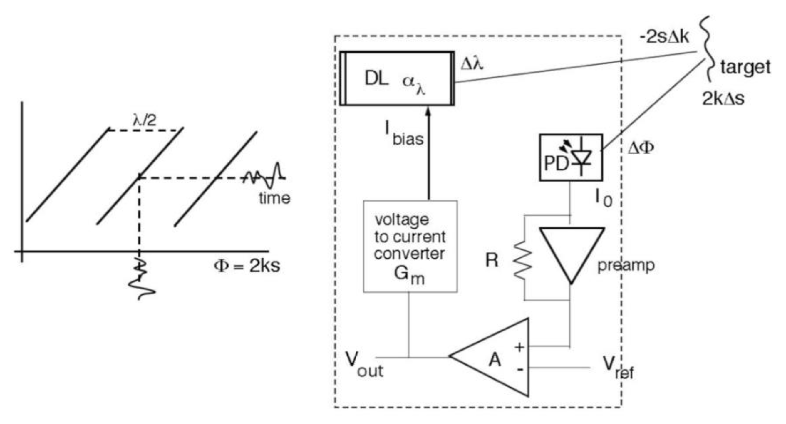
Refurbishing the HFS interferometer with the SMI concept is not straightforward because the SMI has just one arm, i.e., no reference arm is available to be actuated. However, the use of a laser diode as the source of the SMI brings about the advantage (in this case) of wavelength λ being dependent on bias current I_bias through a coefficient α_λ = dλ/dI_bias.

Then, the optical phaseshift variation Δϕ = Δ(2ks) = 2(sΔk + kΔs) can be dynamically kept equal to zero by making sΔk = −kΔs, where Δk = −2πΔλ/λ² and Δλ is obtained using the change in bias current as Δλ = α_λΔI_bias [34,35]. To complete the feedback loop, we have a voltage-to-current drive of bias current, I_bias = G_mV_out, and the amplified signal of the photodiode, from which the level V_hf of the half-fringe is subtracted.

A scheme showing the feedback loop of such an HFS SMI is presented in Figure 10. It has two ‘virtual ground nodes’ with functionality similar to the virtual ground of an operational amplifier: the phase node, where ϕ = sΔk + kΔs ≈ 0, and the difference amplifier inputs, where V_in − V_hf ≈ 0 (where V_hf is the level of half-fringe). With the notation ≈0, we indicate that the signals are kept dynamically very small, at a level just enough to be amplified and generate the desired amplitudes along the loop.

From the condition sΔk + kΔs = 0, where k = 2π/λ, we obtain Δs/s = Δλ/λ. After inspection of the feedback loop in Figure 10, we can write Δλ = I_biasα_λ = V_outα_λG_m, and substituting in Δs, the signal voltage is found as V_out = (s/λα_λG_m)Δs.

An important consequence is that the response factor s/λα_λG_m is independent of the optical power carrying the signal—provided the loop gain G_loop is large enough.

Indeed, the loop gain of the scheme in Figure 10 is easily seen to be G_loop = 2ks I₀ RAG_m (α_λ/λ), and its value can be made G_loop ≈ 10³ in practice.

Thus, as it is well known from the general properties of feedback, all sources of disturbances and deviation from linearity are reduced by a factor given by the loop gain plus one, or ≈10³. In particular, unexpectedly, speckle pattern fluctuations of the signal amplitude are washed out and absorbed by the loop gain.

The nonlinearity is also very important due to the λ/2 fringe amplitude being affected. The resulting dynamic range is no longer λ/2 of the plain interferometer, but it is now (1 + G_loop)λ/2, or a fraction of an mm instead of a fraction of a μm.

Qualitatively, this result is explained considering that as the Δs signal increases and tends to escape out of the λ/2 width of the fringe, the feedback action pulls it back to the middle of the fringe—so a much larger amplitude (1 + G_loop)λ/2 is necessary to finally reach the boundary of the dynamic range.

Because of the same mechanism, the linearity error is reduced by (1 + G_loop), and for a signal amplitude of half the dynamic range ΔΦ = ±2kΔs = ±45 degrees (or Δs = ±(π/4)/2k = λ/16≈ ±50 nm for λ = 800 nm, which becomes (1 + G_loop)λ/16 ≈ ±50 μm with feedback, that is, 100 μm peak-to-peak), we have a linearity error e_l = (π/4 − sin π/4)/2k = 0.078λ/12.56 = 0.0062 800 nm = 4.96 nm, a record result (=0.005%) for such a large 100 μm signal.

Regarding the minimum measurable displacement or NED (noise-equivalent displacement), this is due to the quantum noise i_n of the beam carrying the phase signal 2kΔs and is given [34,35] by NED = (λ/4π)(I₀/i_n) = (λ/4π) (2eB/I₀)^1/2, where I₀ is the detected current and B is the measurement bandwidth, with typical values of 20 to 100 pm/√Hz in practice [34].

A totally different method to linearize the response of the SMI has been recently introduced [36], and the method is based on working under the strong feedback (or high C) regime. Indeed, at large C (say, 10 … 20) the amplitude of fringes is found to decrease while increasing intervals of the SMI waveform are dragged by the target displacement s(t), until at a certain C_min, the fringes disappear and the SMI signal is just a replica of Δs(t). At still larger C = C_max, however, the system enters the bifurcation regime, and period-1 chaotic oscillations are generated [30]. Thus, we shall adjust the feedback parameter C to stay in the interval C_min < C < C_max, typically 10 to 30. The drawback of the method is that the C-interval depends on the amplitude of the phase signal kΔs, on the stand-off distance s and on the drive current I_bias [36], so it is difficult to accommodate a large dynamic range of signals kΔs.

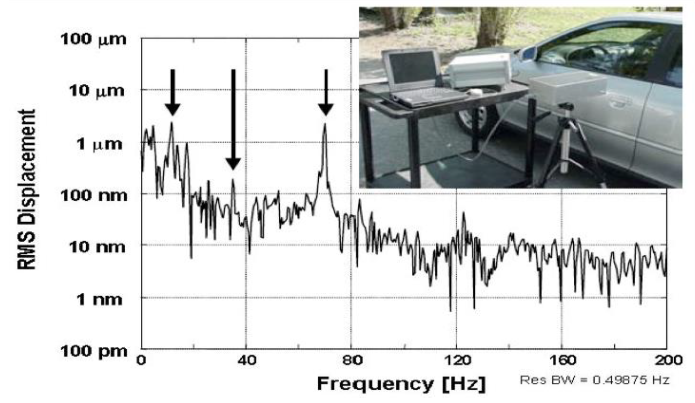
4.1. Measuring Vibration Modes with the HFS SMI

Thanks to the wide dynamic range extending for several decades, e.g., from ≈50 pm to ≥500 μm, the good linearity in the response, and the substantial bandwidth (typically several hundred kHz), the HFS SMI can easily supply the spectrum of modes of a mechanical structure. An example is provided in Figure 11, where we report the frequency spectrum of the SMI signal (V_out of Figure 10) obtained when pointing the device at the door of a car with the motor engine running. A complicated set of vibration modes of the structure is unveiled by the SMI measurement.

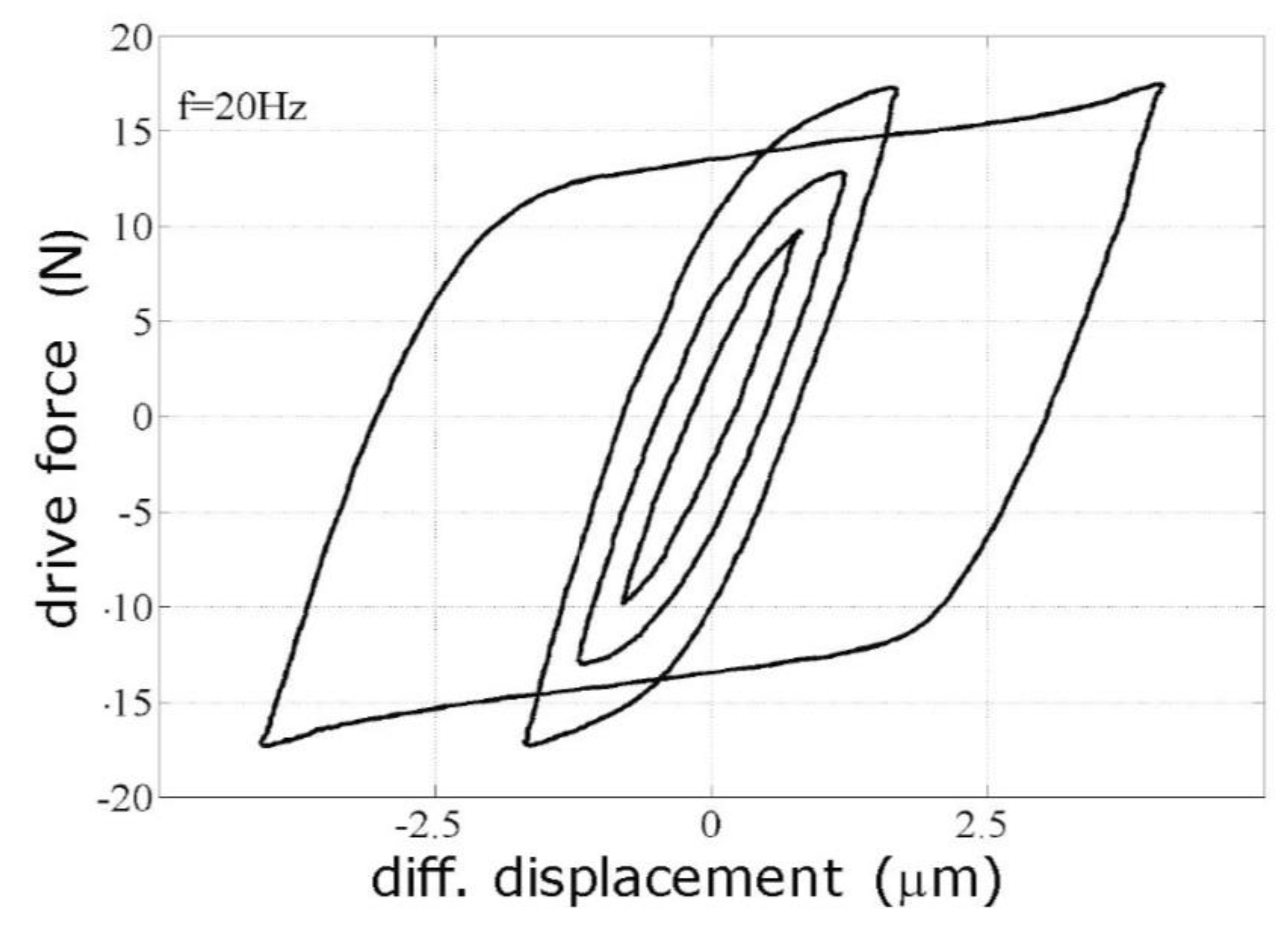
4.2. Measuring Mechanical Hysteresis with a Differential HFS SMI

The SMI can be made quasi-differential by pairing two HFS units and making the difference be their output signals [34].

The difference V_out1 − V_out2 is not exactly the same as the difference of phases ϕ₁ − ϕ₂ = 2k(s₁ − s₂) made by the superposition of measurement and reference beams in a normal LI. However, it closely approaches it inasmuch as V_out is linearly related to Δs, like in an HFS interferometer.

For best results, the noise and dynamic range of two HFS SMIs shall be matched within 5%, and then a weighted subtraction V_out1 − ηV_out2 is made, adjusting the weight η so that when the two units are aimed just to the same point, the difference in the outputs is <10⁻³ of the single component output.

Then, the differential SMI can be applied to the measurement of a small sample, for example, a bead of a motor damper, subjected to a vibratory stress (one unit) and to the base holding the object (the other unit). In this way, we have (i) a common mode signal, proportional to the applied stress (or force per unit area) and (ii) a differential signal proportional to the strain (or relative deformation) imparted to the sample.

The result is shown in Figure 12. Note that the measurement of the hysteresis cycle supplies an important design tool because it allows for selecting the right level of stress to maximize the power dissipated by the damper (given by the area of the cycle times the frequency of operation) while keeping a safe margin to avoid breakdown of the sample.

For more information on the HFS method, the reader may consult Refs. [34,35,37], and Ref. [38] that reports the complete performances of a commercial vibrometer inspired by the research described in this Section.

4.3. Measuring Acoustic Emission with the High-C Linearized SMI

The high-C linearized SMI has been successfully used to measure the AE (acoustic emission) from an aluminum rectangular plate excited with a small piezo placed on the edge of the plate, where the SMI sensor was a fiber-pigtailed DFB laser [36]. The sensing length of the fiber, glued to the Al plate, was 15 cm, and the total (standoff) fiber length was 1.50 m. At f = 40 kHz of excitation, the SMI vibration sensor was able to detect 14 με of strain (where ε = Δl/l is the strain unit), corresponding to an amplitude of 2.12 μm, and it had a noise-limited sensitivity of 0.25 nε/√Hz [36].

5. Switching Cancellation (SC) Analog Readout SMI Vibrometer

A simple yet effective method for reconstructing the SMI waveform under the moderate feedback regime (1 < C < 4.6) was introduced in Ref. [39], which was developed for the measurement of vibrations and oscillation mode of medium-size structures (say, a few meters in size) in Ref. [40]. It starts from the observation that, if we remove the switching steps in the SMI signal I = I₀ cos 2ks(t), after sliding the waveform to restore its continuity, the result is practically coincident with the drive waveform s(t) (see Figure 5 in Ref. [39]).

To implement this concept, called switching cancellation (SC), we first time-differentiate the SMI signal to obtain a sequence of positive and negative pulses in correspondence with the upgoing and down-going switching, then separate the positive and negative pulses and send them to a stretcher circuit supplying a step waveform slowly decaying in time (to avoid a pile-up of tails), and then subtract the steps to the SMI signal, thus removing the switching.

Theoretically, this procedure is difficult to analyze and justify. However, heuristically, it proves to be robust and fairly accurate in the moderate feedback range because the error of reconstruction is just a little fast ripple easily filtered out using a low-pass operation.

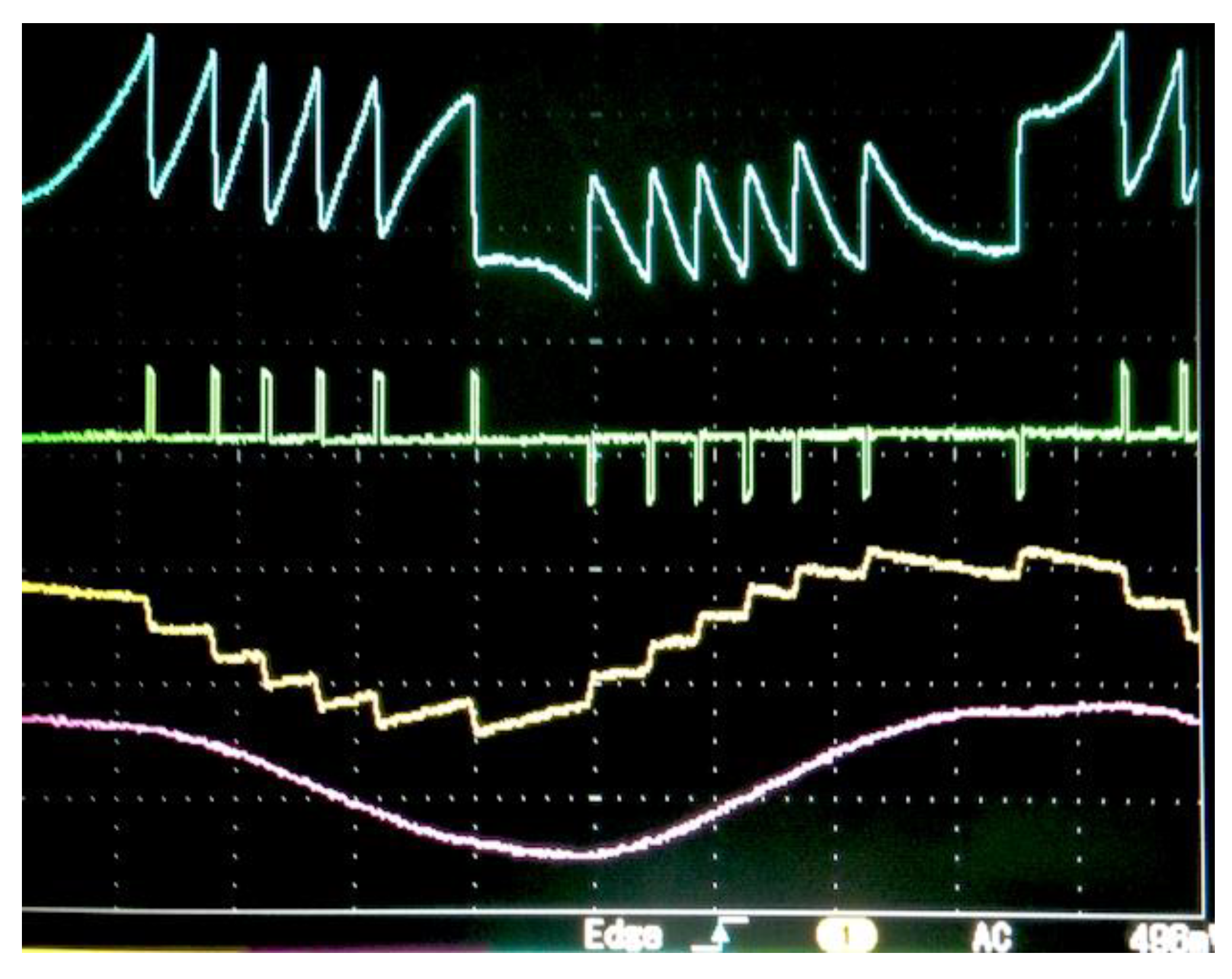
An example of waveforms obtained using the SC circuit is shown in Figure 13. Here, a loudspeaker with a cone covered with untreated white paper was used as the diffusive target. It was driven with a sine wave, yielding a peak-to-peak signal amplitude of 5 μm at 20 Hz; the wavelength of the laser was 780 nm, and the feedback factor was estimated to be C ≈ 3. Similar waveforms were also observed for peak-to-peak signal amplitudes from 400 nm to 20 μm, in a range of frequency going from 0.1 Hz to 100 Hz [40].

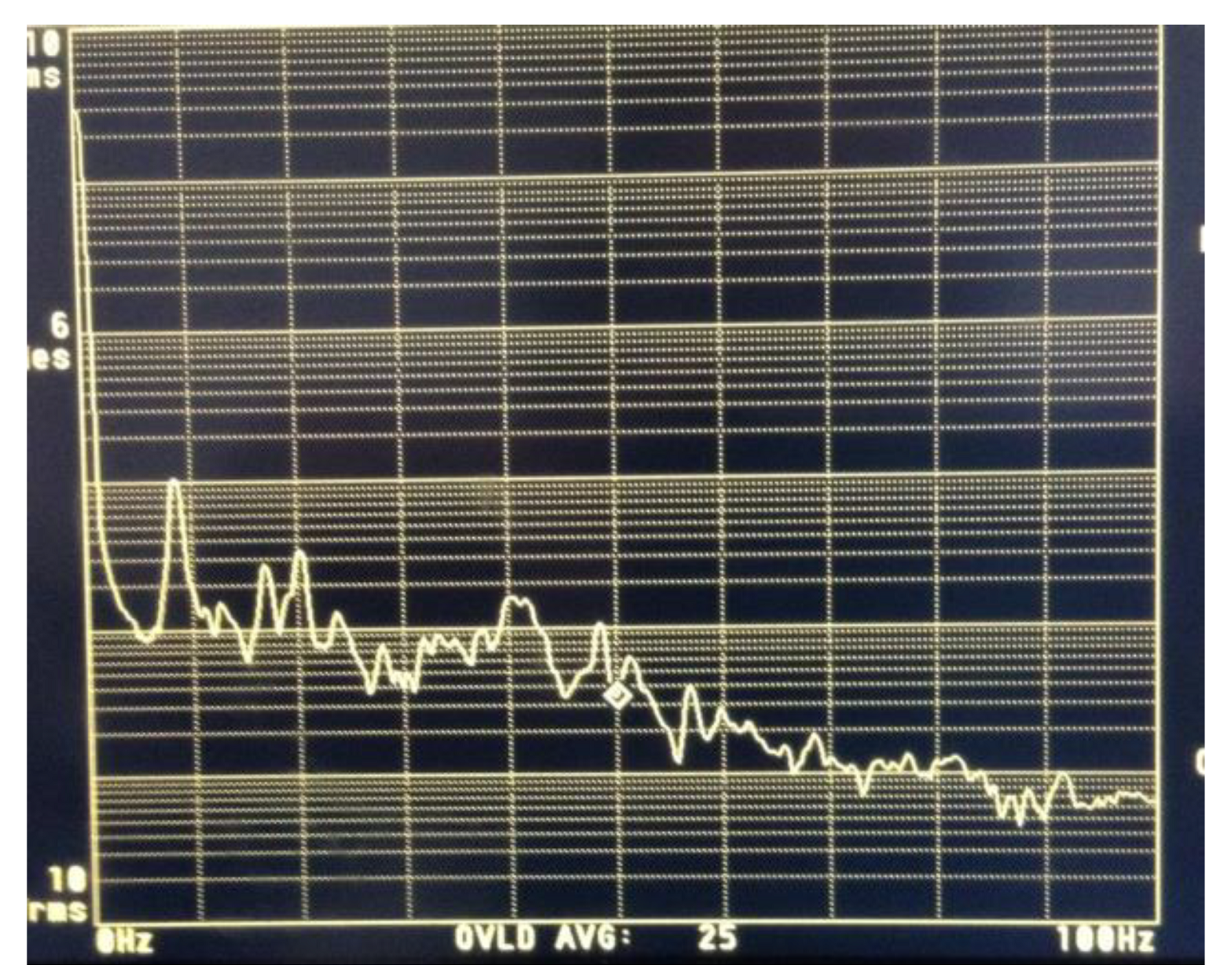
Observing the SMI reconstructed signal at the (electrical) spectrum analyzer reveals the ambient-related vibrations collected using the setup and, adding an excitation, the vibration modes of the structure. As an example, by pointing the beam of the SC-SMI at the floor when placed on an anti-vibration table at 1.2 m height, we were able to measure the spectrum of the vibrations collected by the floor, as reported in Figure 14.

The SC-SMI vibrometer is simple and easy to use and works well on untreated target surfaces. Its performance is limited by the circuits handling the SMI signal and covering the middle-to-high range of amplitudes, that is, from ≈0.5 μm to ≈50 μm, and the frequency components from 0.1 to 100 Hz.

A potential application of this version SC-SMI of the vibration analyzer is the low-cost intrusion detector for approaching persons.

6. Frequency-Shifted (FS) Long Standoff Distance Vibrometer (LI and SMI)

Testing large structures using a laser vibrometer is an application that was developed soon after the advent of the laser. Since the 1980s, He-Ne-based instruments have been extensively used in the field [41,42,43] for the remote (standoff distance of ≈100 m) monitoring of structures like dams and towers [44].

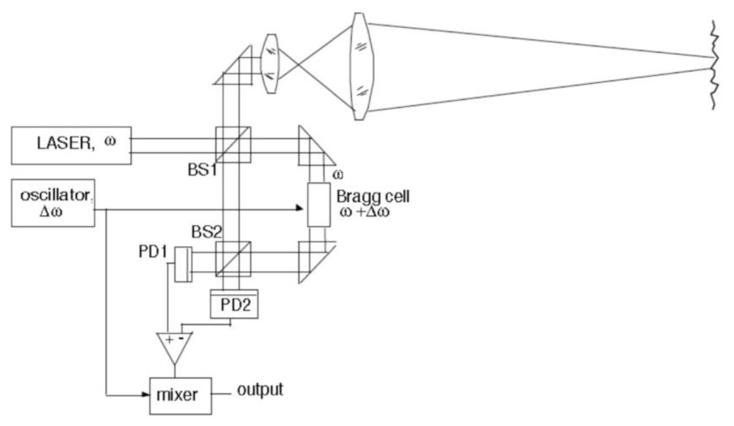
The most viable and commonly accepted approach to build a single-channel (i.e., yielding a cos 2ks signal) laser interferometer yielding a long standoff distance and nm-capability is the frequency-shifted (FS) approach, in connection with a frequency stabilized laser (to attain a long coherence length).

The shift is obtained by a Bragg acousto-optic cell, which allows the signal 2ks(t) to be impressed on a carrier frequency of 20–50 MHz so that by demodulating the received signal, we can trace back the small vibration s(t) [45]. This operation is carried out using the arrangement shown in Figure 15.

The source is a laser stabilized in frequency so that the linewidth (typ. Δν = 100 kHz) is narrow enough to give interference after the long (2 s = 200 m, typically) propagation path to the remote target and back, and the wavelength is chosen in correspondence with atmospheric minima of absorption [45]. The He-Ne is a good choice along with the CO₂ laser at λ = 10.6 μm for better transmission through haze.

Recently, the GaAlAs diode laser (grating stabilized for low Δν) was used in connection with the SMI version of the vibrometer. This is obtained simply by placing the Bragg cell of Figure 15 along the propagation path to the target.

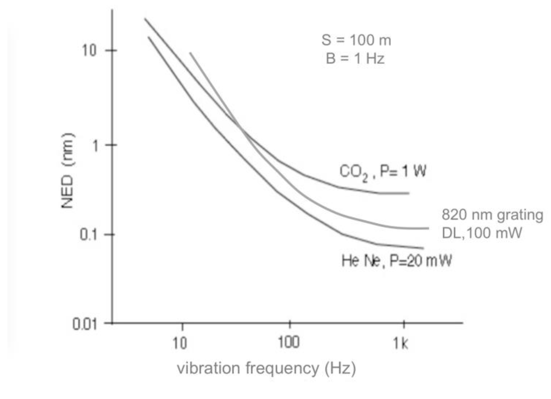
Regarding the minimum detectable displacement (or NED), this is determined by the quantum noise of the detected return and eventually by the limited coherence length, with a usually substantial contribution of the 1/f component. As we can see from Figure 16, the NED for a CO₂ laser is better than that of a He-Ne, and both are comparable to the GaAlAs laser diode in the SMI configuration.

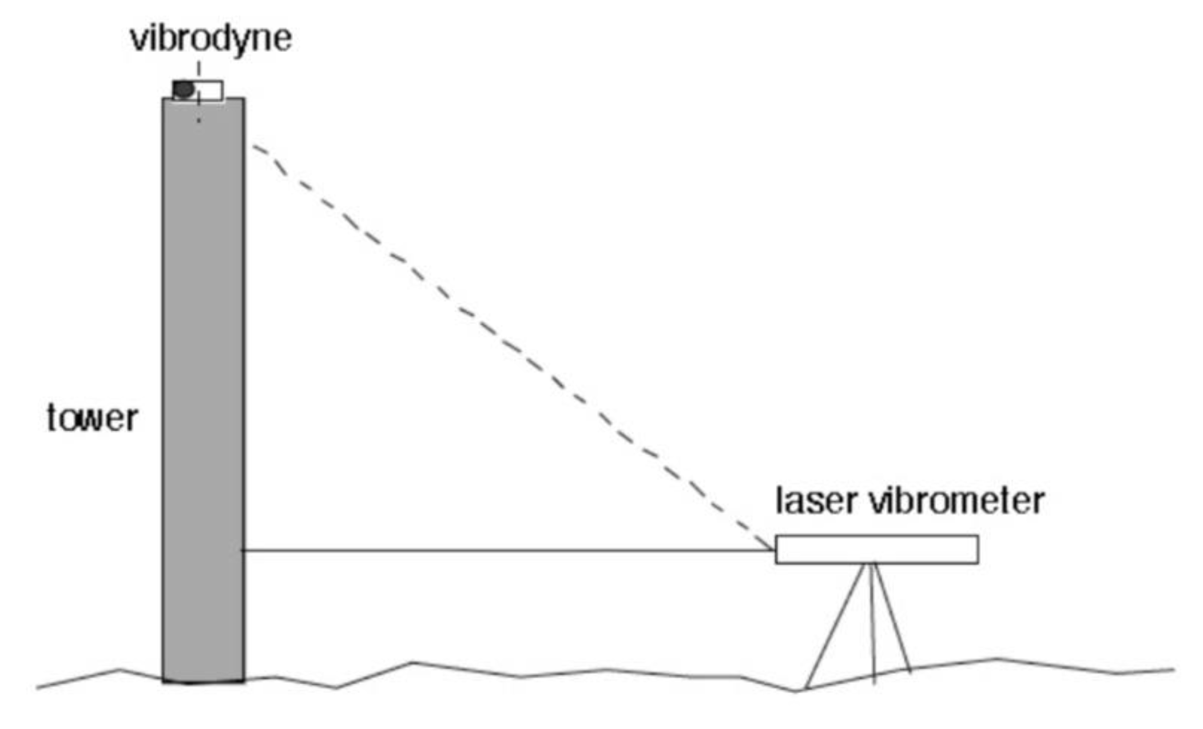
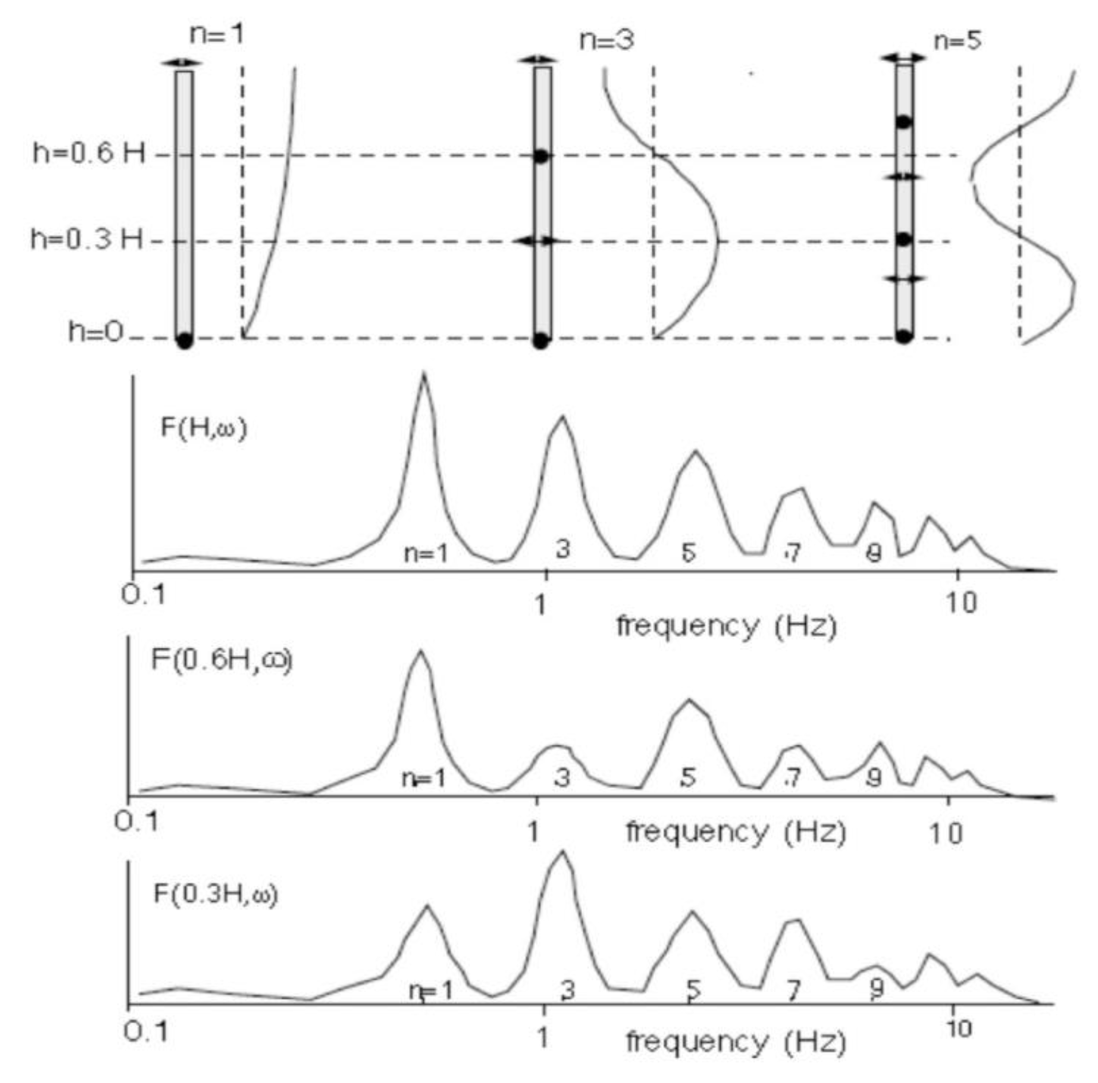
The long-distance vibrometer is useful for detecting the vibration mode and frequency response of a large structure, for example, a tower, as shown in Figure 17.

Here, a vibrodyne—a rotating motor with an eccentric-mounted mass—is mounted atop the tower and scanned in frequency to measure the frequency response, as shown in Figure 18.

The laser vibrometer scans spots at selected heights of the tower, and the result is a chart showing responses that the structural engineer can interpret to diagnose the integrity of the structure.

7. Speckle Pattern Errors

As native targets are usually diffusive surfaces, the field returning to the measuring port (either the beamsplitter of the LI or the DL of the SMI) is subject to well-known speckle pattern statistics [46,47,48,49,50,51].

Speckle statistics bring about measurement error, and we can consider circumventing it using a mirror as the target. However, this option is to be absolutely avoided because it is invasive and requires a clumsy alignment operation. Using a corner cube [52] eliminates the alignment but aggravates the invasiveness, so it is never used in practice, except in displacement measurements with tool machines because it can be fastened to the moving turret. A retroreflector tape (or varnish) over the native surface can be used to obtain an increase in the retroreflected power by a factor of 20 to 50, together with the mitigation of speckle errors and the alignment requisite. Yet, the retroreflector tape is also invasive, and we should possibly avoid it when working on the native, diffusive surface of the target.

On a diffusive surface, speckle statistics [46,47,48] are generated by the randomness, at the λ-scale, of the height of individual elemental areas illuminated with the incoming laser spot. As a result, both the amplitude and phase of the field returning to the measuring port fluctuate (or have an error) because of the speckle noise, both in LI and SMI.

The statistics of speckle intensity is a negative exponential with a decay constant equal to the average value: that of amplitude is a Rayleigh distribution, and that of phase is a uniform distribution over 0–2π [46,47,48].

Given the point-wise nature of the vibration measurement, amplitude fluctuation is easily cured. If we unfortunately fall on a dark speckle giving back a signal amplitude much less than the average, we simply move the aim of the beam away and find another spot nearby where the amplitude is larger and sufficient.

An SMI with BST (bright speckle tracking) was developed [49] to cure amplitude fading. Also, remarkably, the HFS SMI can bear a substantial attenuation of speckle amplitude thanks to the feedback loop gain, but all the other LI and SMI schemes are subject to full speckle amplitude fading.

On the other hand, the phase error entirely impacts the measurement because theoretically, we cannot distinguish it from the useful phase signal ϕ = 2ks.

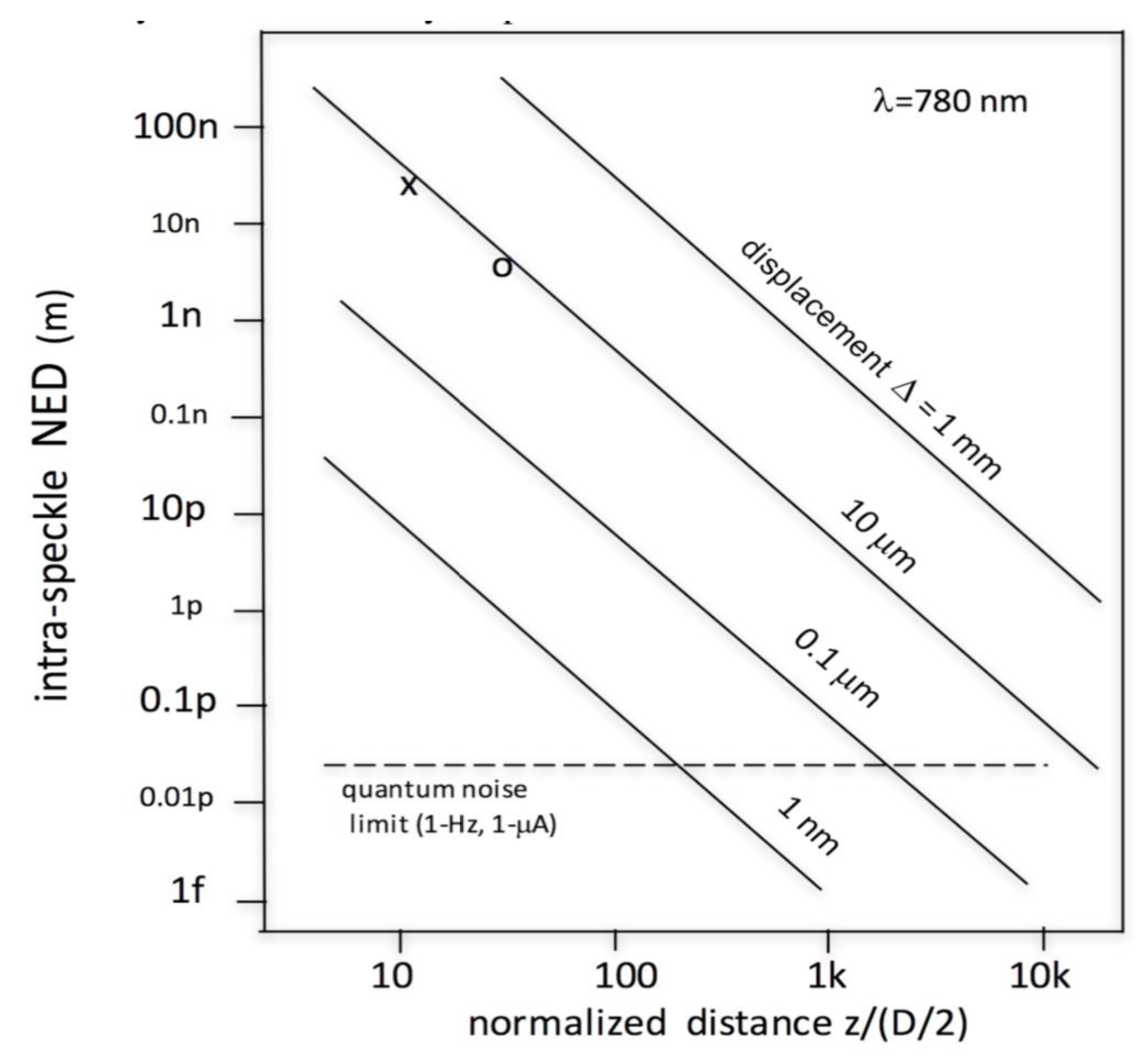
An analysis of the phenomenon shows that the phase error can be reduced by making the spot size as small as possible because the phase-induced error (or NED, noise equivalent displacement) is given by [46,47,48,49,50] NED = (C/4√2)Δ(D/2z)², where Δ is the amplitude of the vibration, D is the spot diameter, z is the target distance, and C/4√2 is a multiplicative factor not much different from one. In Figure 19, we plot the NED as a function of normalized distance z/(D/2). As we can see, the nose contribution can become even smaller than the quantum noise of the beam (for a detected current of 1 μA) for z > (≈200) (D/2), that is, for z = 100 mm when D = 1 mm.

8. Discussion and Conclusions

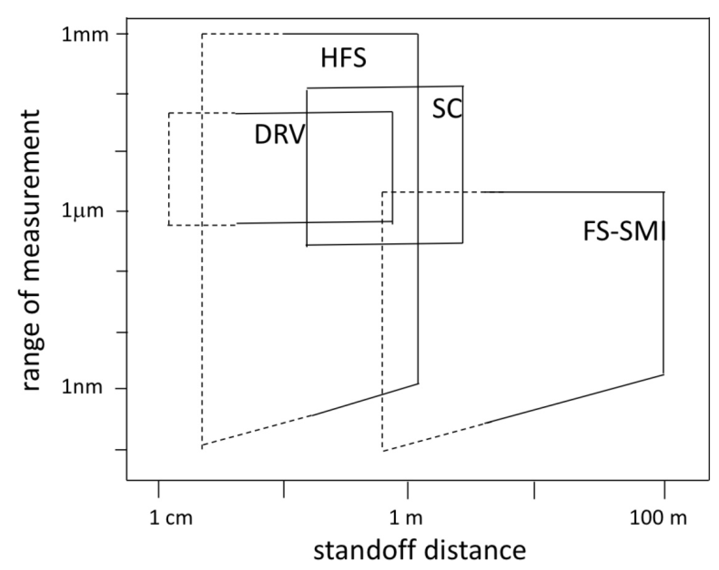
In Figure 20, we summarize the typical performances of SMI vibrometers described in the previous Sections with regard to the covered measurement range and standoff distance.

These results demonstrate the suitability of SMI techniques for non-invasive, contactless measurement of vibrations and for assessing the parameters of a mechanical system, all with the fine spatial resolution determined by the laser spot size.

The reported approaches offer case studies and guidelines to develop vibration measurements spanning from tens of picometer to millimeters in amplitude and sub-Hz to MHz in frequency, with a variety of standoff distances. Thus, they provide a benchmark and a guide for anyone entering the field of vibration measurement of kinematic quantities.

Vibrations are also called for in several other fields of science and technology, for example, in biomedical sensing, structural testing, and seismology, where they are still in their infancy but may lead soon to important breakthroughs, an important event for all researchers interested in the field. In all the techniques described, the SMI configuration demonstrates itself as particularly simple and low-cost, while supplying a high sensitivity of detection and fast response.

Regarding the development of new ideas in SMI, a crucial caveat to bear in mind is that, given the advantages of the simple starting configuration, one with low cost and minimum part count, any added expensive component should be carefully avoided, as well as avoiding heavy computer resources. In other words, adding components to the SMI destroys the inherent simplicity of the configuration and is not at all advisable.

Also, the operation should be on diffusive targets (not mirrors or other components attached to the target or part of the setup) to maintain the non-invasiveness and non-contact remote mode of operation.