

Uncertainty Propagation and Global Sensitivity Analysis of a Surface Acoustic Wave Gas Sensor Using Finite Elements and Sparse Polynomial Chaos Expansions
Abstract
:1. Introduction
2. Simulation Model
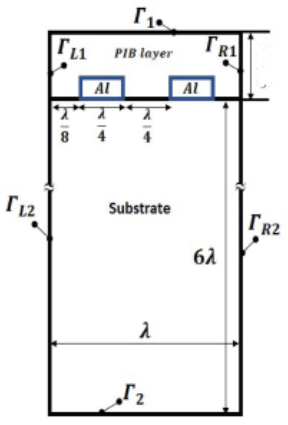
2.1. Geometry
2.2. Sensing Model
2.3. Material Properties
2.4. Boundary Conditions
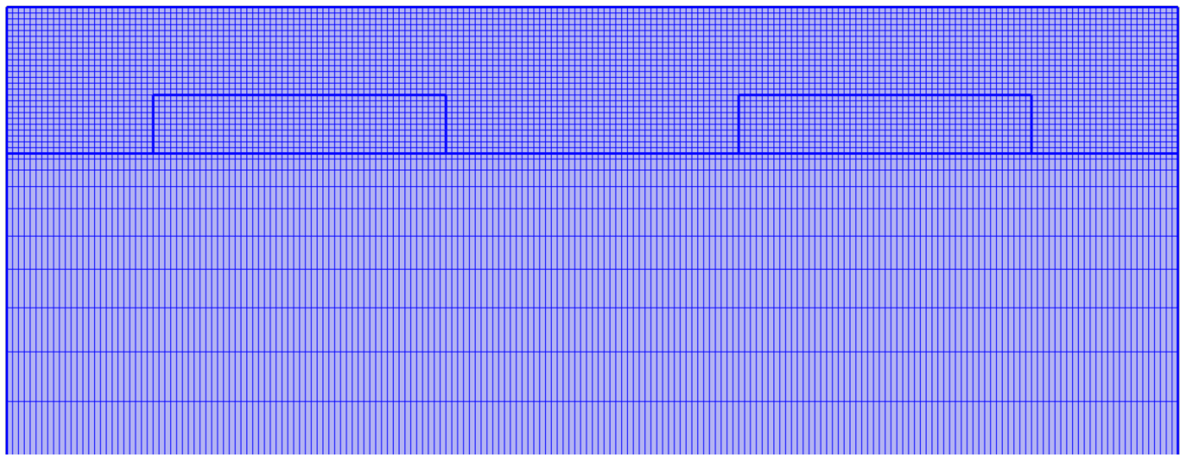
2.5. Mesh
2.6. Sensor Sensitivity
3. Uncertainty Propagation (UP)
4. Global Sensitivity Analysis (GSA)
4.1. Generalities
4.2. Sobol’ Indices
- The term is equal to the expected value of ;
- The expected value of the summands with respect to their own variables in (4) is equal to zero.
5. Sparse Polynomial Chaos Expansions
5.1. Polynomial Chaos Expansion
5.2. Sparse Least Squares Coefficients Computation
5.3. Sobol’ Indices Computation
5.4. Steps for Uncertainty Propagation and Global Sensitivity Analysis with Sparse Polynomial Chaos
- Form a DoCE by choosing appropriate design points of the multi-variate parameter space by a suitable sampling method (Monte Carlo, LHS, Sobol sequence, Halton sequence, etc.);
- Evaluate the computational model at these points and obtain the model responses ;
- Compute the polynomial chaos coefficients using sparse least squares (LAR or OMP algorithms);
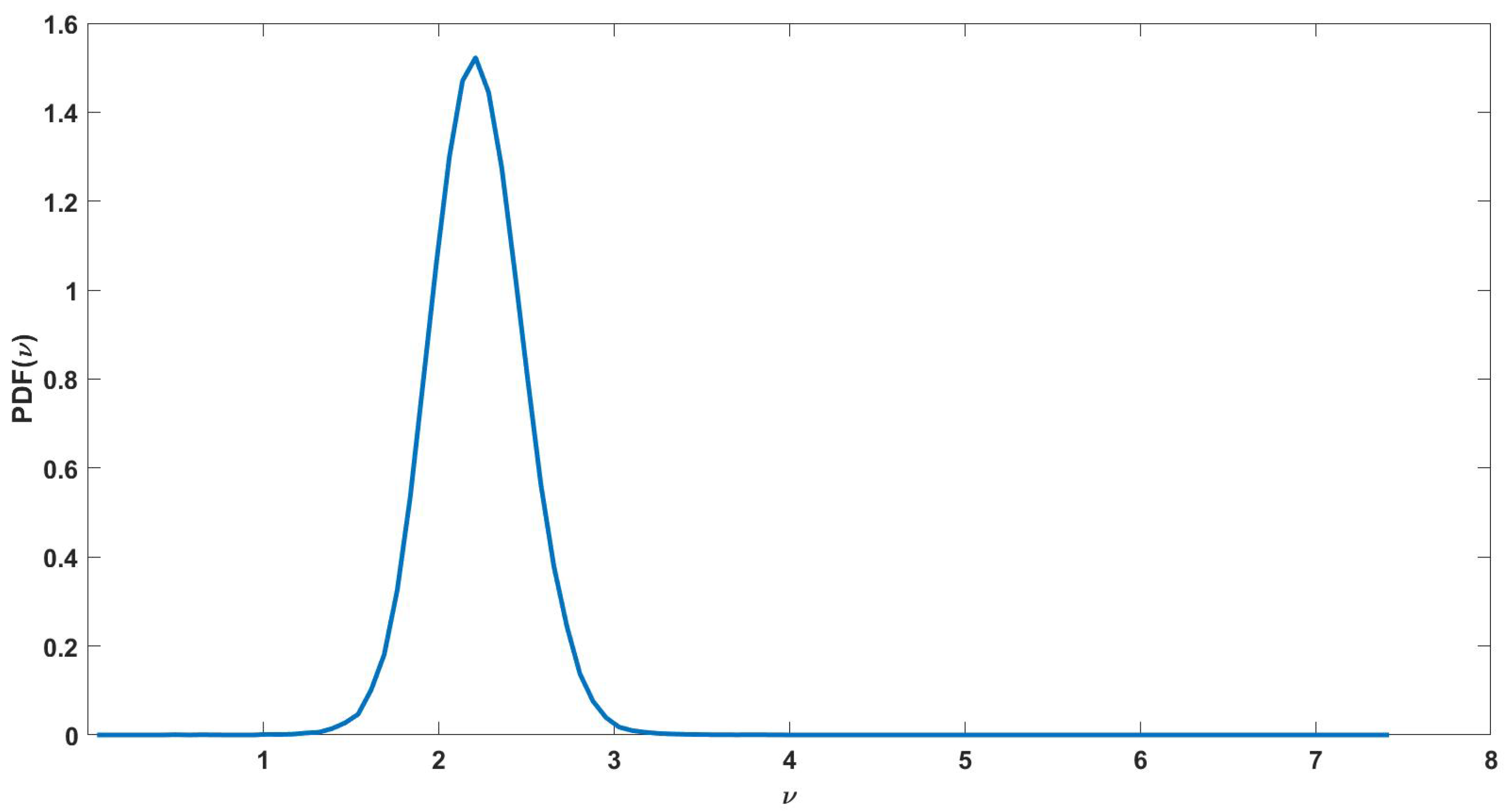
- Use the polynomial chaos expansion to determine mean, variance, higher order moments and density of the output;
- Compute total Sobol’ indices for each variable using (19).
6. Results
6.1. Model Validation
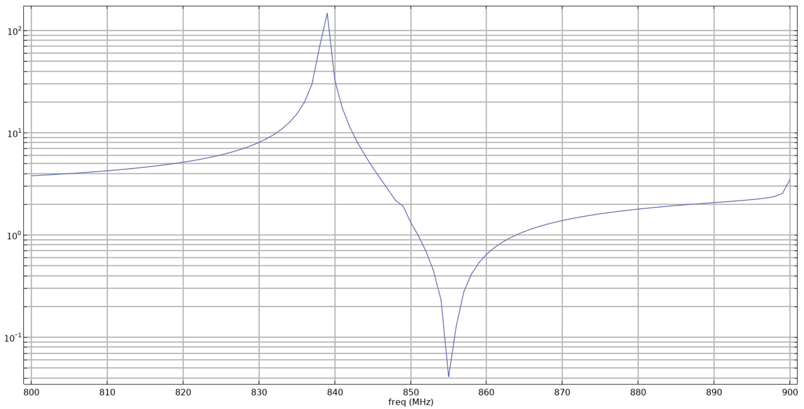
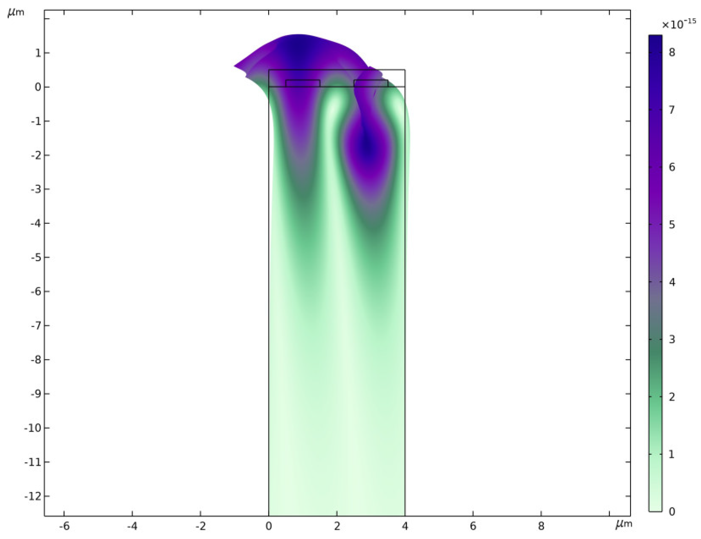
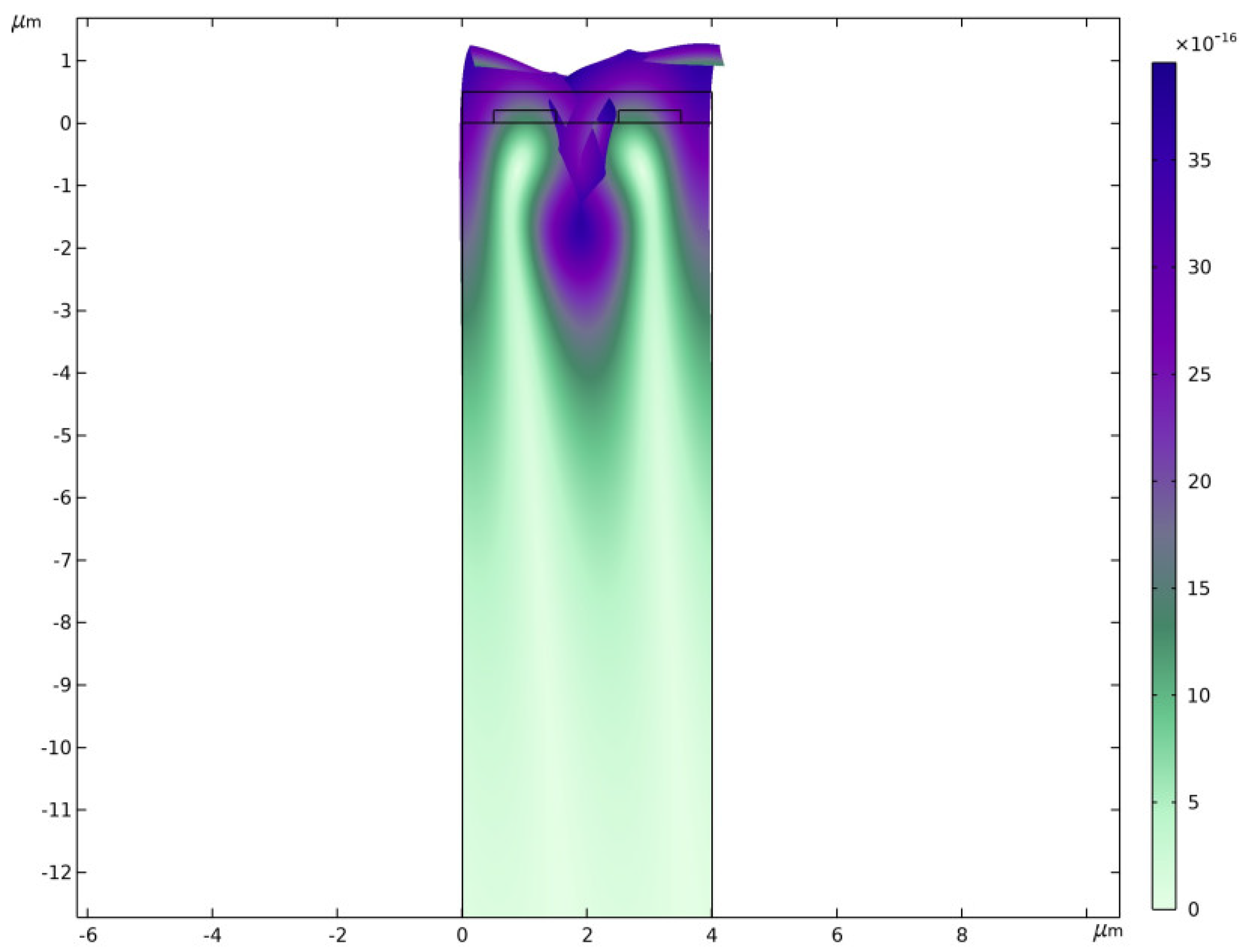
6.2. SAW Modes and Resonant Frequencies
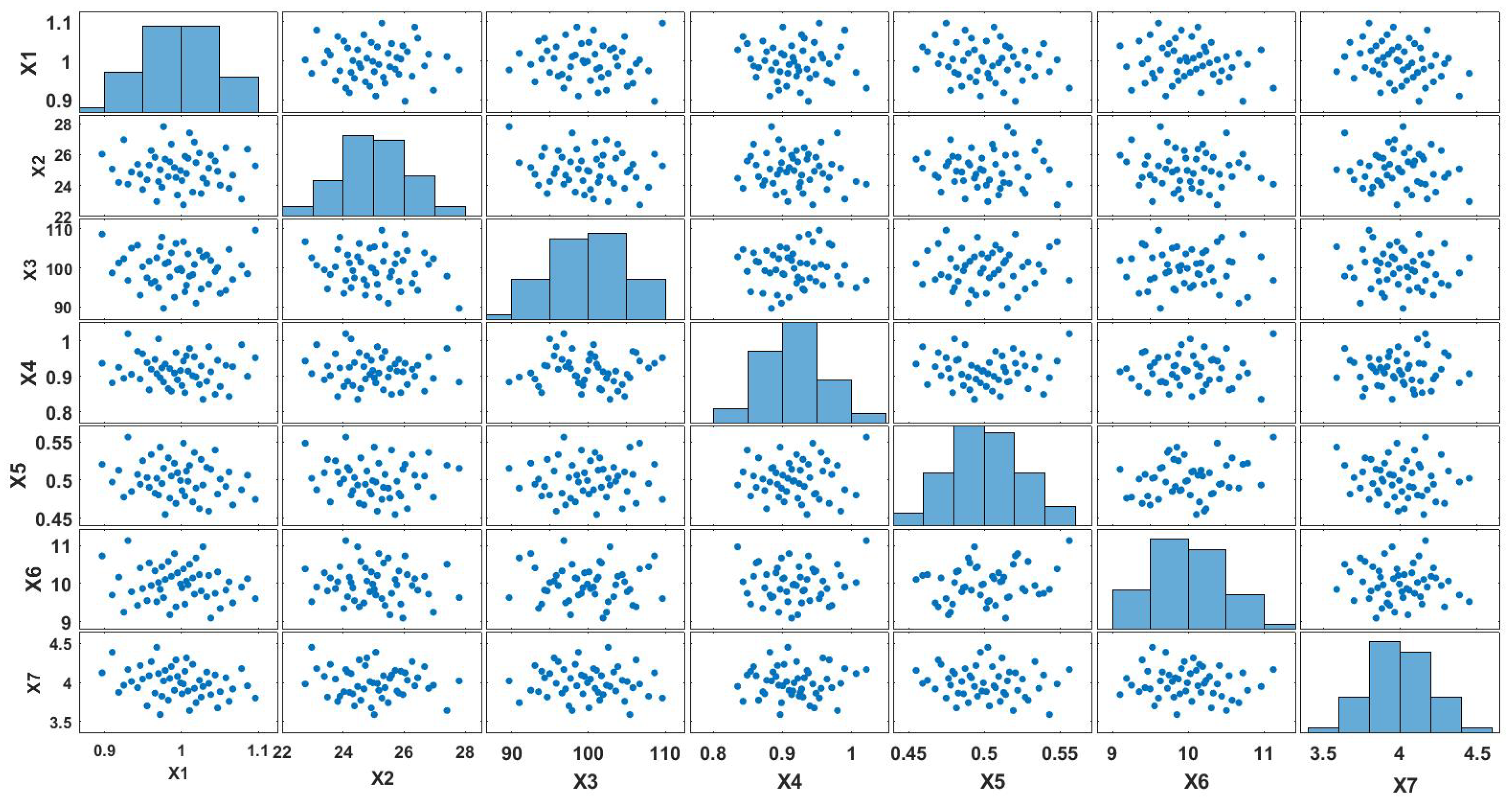
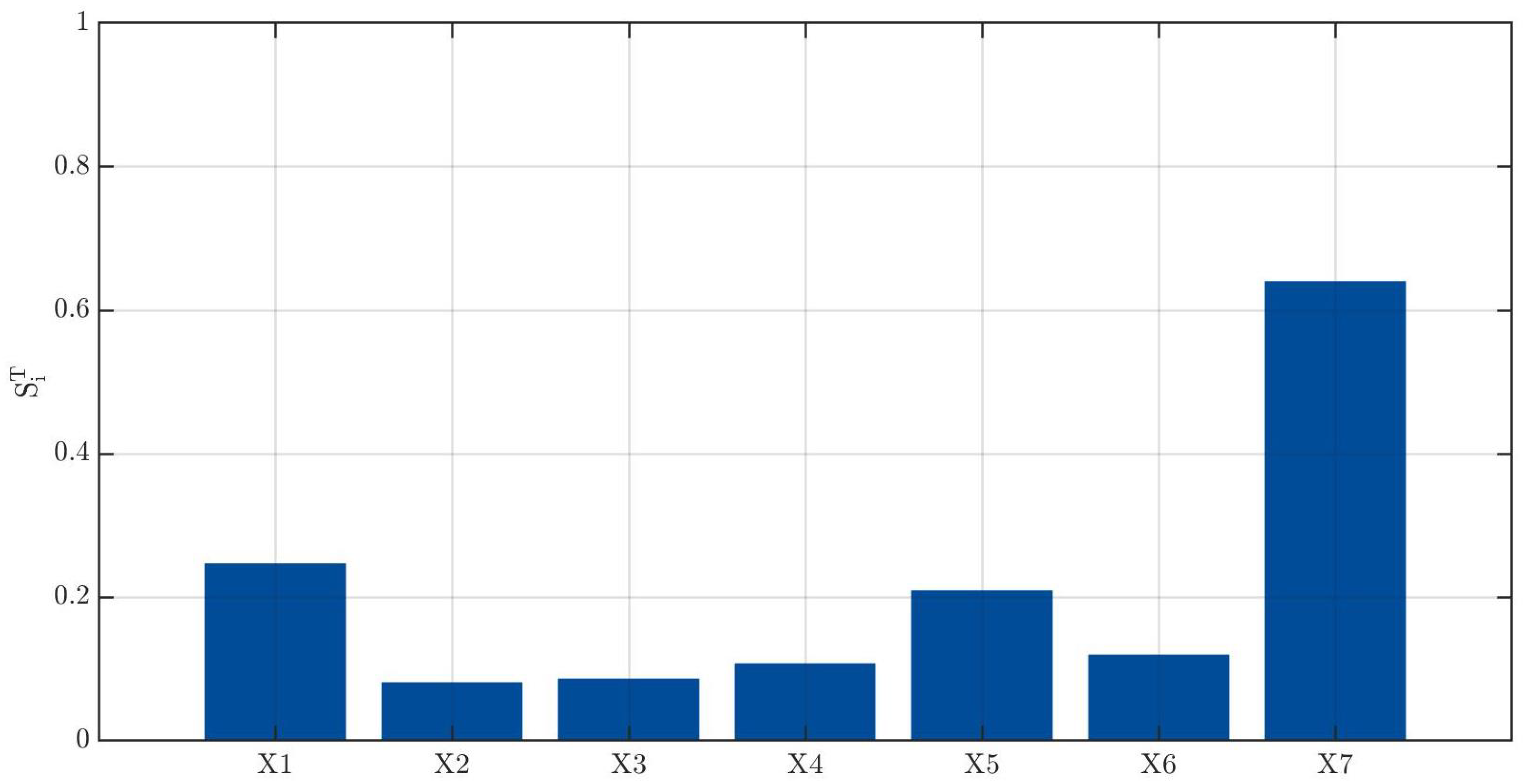
6.3. Global Sensitivity Analysis
6.3.1. Low Input Variability
6.3.2. Medium Input Variability
7. Conclusions
Funding
Acknowledgments
Conflicts of Interest
References
- Rayleigh, L. On waves propagated along the plane surface of an elastic solid. Proc. Lond. Math. Soc. 1885, s1-17, 4–11. [Google Scholar] [CrossRef]
- Jakubik, W.P. Surface acoustic wave-based gas sensors. Thin Solid Films 2011, 520, 986–993. [Google Scholar] [CrossRef]
- White, R.M.; Voltmer, F.W. Direct piezoelectric coupling to surface elastic waves. Appl. Phys. Lett. 1965, 7, 314–316. [Google Scholar] [CrossRef]
- Vellekoop, M. Acoustic wave sensors and their technology. Ultrasonics 1998, 36, 7–14. [Google Scholar] [CrossRef]
- Thompson, M.; Stone, D.C. Surface-Launched Acoustic Wave Sensors: Chemical Sensing and Thin-Film Characterization; Wiley-Interscience: Hoboken, NJ, USA, 1997; Volume 144. [Google Scholar]
- D’Amico, A.; Palma, A.; Verona, E. Hydrogen sensor using a palladium coated surface acoustic wave delay-line. In Proceedings of the 1982 Ultrasonics Symposium, San Diego, CA, USA, 27–29 October 1982; pp. 308–311. [Google Scholar] [CrossRef]
- Galipeau, J.; LeGore, L.; Snow, K.; Caron, J.; Vetelino, J.; Andle, J. The integration of a chemiresistive film overlay with a surface acoustic wave microsensor. Sens. Actuators B Chem. 1996, 35, 158–163. [Google Scholar] [CrossRef]
- Urbańczyk, M.; Jakubik, W.; Kochowski, S. Investigation of sensor properties of copper phthalocyanine with the use of surface acoustic waves. Sens. Actuators B Chem. 1994, 22, 133–137. [Google Scholar] [CrossRef]
- Yu, R.; Niu, S.; Pan, C.; Wang, Z. Piezotronic effect enhanced performance of Schottky-contacted optical, gas, chemical and biological nanosensors. Nano Energy 2015, 14, 312–339. [Google Scholar] [CrossRef] [Green Version]
- Seh, H.; Hyodo, T.; Tuller, H. Bulk acoustic wave resonator as a sensing platform for NOx at high temperatures. Sens. Actuators B Chem. 2005, 108, 547–552. [Google Scholar] [CrossRef]
- Chen, C.; Jiang, M.; Luo, X.; Tai, H.; Jiang, Y.; Yang, M.; Xie, G.; Su, Y. Ni-Co-P hollow nanobricks enabled humidity sensor for respiratory analysis and human-machine interfacing. Sens. Actuators B Chem. 2022, 370, 132441. [Google Scholar] [CrossRef]
- Wang, S.; Xie, G.; Su, Y.; Su, L.; Zhang, Q.; Du, H.; Tai, H.; Jiang, Y. Reduced graphene oxide-polyethylene oxide composite films for humidity sensing via quartz crystal microbalance. Sens. Actuators B Chem. 2018, 255, 2203–2210. [Google Scholar] [CrossRef]
- Su, Y.; Chen, S.; Liu, B.; Lu, H.; Luo, X.; Chen, C.; Li, W.; Long, Y.; Tai, H.; Xie, G.; et al. Maxwell displacement current induced wireless self-powered gas sensor array. Mater. Today Phys. 2023, 30, 100951. [Google Scholar]
- Estill, C.F.; Spencer, A.B. Case study: Control of methylene chloride exposures during furniture stripping. Am. Ind. Hyg. Assoc. J. 1996, 57, 43–49. [Google Scholar] [CrossRef]
- Li, S.; Wan, Y.; Su, Y.; Fan, C.; Bhethanabotla, V.R. Gold nanoparticles amplified surface acoustic wave biosensors for immunodetection. In Proceedings of the 2016 IEEE SENSORS, Orlando, FL, USA, 30 October–3 November 2016; pp. 1–3. [Google Scholar] [CrossRef]
- He, S.-T.; Gao, Y.-B.; Shao, J.-Y.; Lu, Y.-Y. Application of saw gas chromatography in the early screening of lung cancer. In Proceedings of the 2015 Symposium on Piezoelectricity, Acoustic Waves, and Device Applications (SPAWDA), Jinan, China, 30 October–2 November 2015; pp. 22–25. [Google Scholar] [CrossRef]
- Joo, B.-S.; Lee, J.-H.; Lee, E.-W.; Song, K.-D.; Lee, D.-D. Polymer film saw sensors for chemical agent detection. In Proceedings of the Conference on Sensing Technology, Palmerston North, New Zealand, 21–23 November 2005; pp. 307–310. [Google Scholar]
- Abraham, N.; Krishnakumar, R.R.; Unni, C.; Philip, D. Simulation studies on the responses of ZnO-CuO/CNT nanocomposite based saw sensor to various volatile organic chemicals. J. Sci. Adv. Mater. Devices 2019, 4, 125–131. [Google Scholar] [CrossRef]
- Kumar, M.; Bhadu, D. Design Performance and Frequency Response Analysis of SAW-Based Sensor for Dichloromethane Gas Sensing Amidst the COVID-19. J. Vib. Eng. Technol. 2021, 9, 725–732. [Google Scholar] [CrossRef]
- Moustafa, M.; Alzoubi, T.; Elnaggar, M.; Laouini, G. Finite element analysis of multilayered ZnO/AIN/Si strucuture saw sensor for efficient VOCs gas detection. Rom. J. Phys. 2021, 66, 607. [Google Scholar]
- Ionescu, V. Design and analysis of a Rayleigh saw resonator for gas detecting applications. Rom. J. Phys. 2015, 60, 502–511. [Google Scholar]
- Hashimoto, K.Y.; Endoh, G.; Yamaguchi, M. Coupling-of-modes modelling for fast and precise simulation of leaky surface acoustic wave devices. In Proceedings of the 1995 IEEE Ultrasonics Symposium. Proceedings. An International Symposium, Seattle, WA, USA, 7–10 November 1995; Volume 1, pp. 251–256. [Google Scholar]
- Tewary, V. Green’s-function method for modeling surface acoustic wave dispersion in anisotropic material systems and determination of material parameters. Wave Motion 2004, 40, 399–412. [Google Scholar] [CrossRef]
- El Gowini, M.M.; Moussa, W.A. A finite element model of a mems-based surface acoustic wave hydrogen sensor. Sensors 2010, 10, 1232–1250. [Google Scholar] [CrossRef] [Green Version]
- Kabir, K.M.M.; Matthews, G.I.; Sabri, Y.M.; Russo, S.P.; Ippolito, S.J.; Bhargava, S.K. Development and experimental verification of a finite element method for accurate analysis of a surface acoustic wave device. Smart Mater. Struct. 2016, 25, 035040. [Google Scholar] [CrossRef]
- Xu, G. Direct finite-element analysis of the frequency response of a lithium niobate saw filter. Smart Mater. Struct. 2000, 9, 973–980. [Google Scholar] [CrossRef]
- Ho, C.K.; Lindgren, E.R.; Rawlinson, K.S.; McGrath, L.K.; Wright, J.L. Development of a surface acoustic wave sensor for in-situ monitoring of volatile organic compounds. Sensors 2003, 3, 236–247. [Google Scholar] [CrossRef] [Green Version]
- Gobet, E. Monte-Carlo Methods and Stochastic Processes: From Linear to Non-Linear; CRC Press: Boca Raton, FL, USA, 2016. [Google Scholar]
- Xiu, D.; Karniadakis, G.E. The wiener–askey polynomial chaos for stochastic differential equations. SIAM J. Sci. Comput. 2002, 24, 619–644. [Google Scholar] [CrossRef]
- Bellman, R.; R Corporation. Adaptive Control Processes: A Guided Tour: R-350; Rand Corporation: Santa Monica, CA, USA, 1961. [Google Scholar]
- Blatman, G. Adaptive Sparse Polynomial Chaos Expansions for Uncertainty Propagation and Sensitivity Analysis. Ph.D. Thesis, Université Blaise Pascal, Clermont-Ferrand, France, 2009. [Google Scholar]
- Blatman, G.; Sudret, B. Adaptive sparse polynomial chaos expansion based on least angle regression. J. Comput. Phys. 2011, 230, 2345–2367. [Google Scholar] [CrossRef]
- Kolda, T.G.; Bader, B.W. Tensor decompositions and applications. SIAM Rev. 2009, 51, 455–500. [Google Scholar] [CrossRef] [Green Version]
- Konakli, K.; Sudret, B. Global sensitivity analysis using low-rank tensor approximations. Reliab. Eng. Syst. Saf. 2016, 156, 64–83. [Google Scholar] [CrossRef] [Green Version]
- Smoliak, S. Quadrature and interpolation formulae on tensor products of certain classes of functions. Dokl. Akad. Nauk SSSR 1963, 148, 1042–1045. [Google Scholar]
- Bungartz, H.-J.; Griebel, M. Sparse grids. Acta Numer. 2004, 13, 147–269. [Google Scholar] [CrossRef]
- Gerstner, T.; Griebel, M. Dimension–adaptive tensor–product quadrature. Computing 2003, 71, 65–87. [Google Scholar] [CrossRef]
- Rehme, M.F.; Franzelin, F.; Pflueger, D. B-splines on sparse grids for surrogates in uncertainty quantification. Reliab. Eng. Syst. Saf. 2021, 209, 107430. [Google Scholar] [CrossRef]
- Iooss, B.; Lemaître, P. A Review on Global Sensitivity Analysis Methods; Springer: Boston, MA, USA, 2015; pp. 101–122. [Google Scholar] [CrossRef] [Green Version]
- Sobol, I. Global sensitivity indices for nonlinear mathematical models and their monte carlo estimates. Math. Comput. Simul. 2001, 55, 271–280. [Google Scholar] [CrossRef]
- Janon, A.; Klein, T.; Lagnoux, A.; Nodet, M.; Prieur, C. Asymptotic normality and efficiency of two Sobol index estimators. ESAIM Probab. Stat. 2014, 18, 342–364. [Google Scholar] [CrossRef] [Green Version]
- Homma, T.; Saltelli, A. Importance measures in global sensitivity analysis of nonlinear models. Reliab. Eng. Syst. Saf. 1996, 52, 1–17. [Google Scholar] [CrossRef]
- Sudret, B. Global sensitivity analysis using polynomial chaos expansions. Reliab. Eng. Syst. Saf. 2008, 93, 964–979. [Google Scholar] [CrossRef]
- Berveiller, M.; Sudret, B.; Lemaire, M. Stochastic finite element: A non intrusive approach by regression. Eur. J. Comput. Mech./Rev. Eur. Méc. Numér. 2006, 15, 81–92. [Google Scholar] [CrossRef] [Green Version]
- Pati, Y.C.; Rezaiifar, R.; Krishnaprasad, P.S. Orthogonal matching pursuit: Recursive function approximation with applications to wavelet decomposition. In Proceedings of the 27th Asilomar Conference on Signals, Systems and Computers, Pacific Grove, CA, USA, 1–3 November 1993; pp. 40–44. [Google Scholar]
- Blatman, G.; Sudret, B. Efficient computation of global sensitivity indices using sparse polynomial chaos expansions. Reliab. Eng. Syst. Saf. 2010, 95, 1216–1229. [Google Scholar] [CrossRef]
- Raghib, A.A.B.M.R.M.; Nordin, A.N. Analysis of electromechanical coupling coefficient of surface acoustic wave resonator in zno piezoelectric thin film structure. In Proceedings of the 2014 Symposium on Design, Test, Integration and Packaging of MEMS/MOEMS (DTIP), Cannes, France, 1–4 April 2014; pp. 1–6. [Google Scholar] [CrossRef]
- Royer, D.; Dieulesaint, E. Elastic Waves in Solids I: Free and Guided Propagation; Springer Science & Business Media: Berlin/Heidelberg, Germany, 1999. [Google Scholar]
- Hadj-Larbi, F.; Serhane, R. Sezawa saw devices: Review of numerical-experimental studies and recent applications. Sens. Actuators A Phys. 2019, 292, 169–197. [Google Scholar] [CrossRef]
- Marelli, S.; Sudret, B. UQLab: A Framework for Uncertainty Quantification in Matlab. In Vulnerability, Uncertainty, and Risk: Quantification, Mitigation, and Management, Proceedings of the Second International Conference on Vulnerability and Risk Analysis and Management (ICVRAM) and the Sixth International Symposium on Uncertainty Modeling and Analysis (ISUMA), Liverpool, UK, 13–16 July 2014; ASCE Library: Reston, VA, USA, 2014; pp. 2554–2563. [Google Scholar] [CrossRef] [Green Version]
- Ricco, A.; Martin, S. Thin metal film characterization and chemical sensors: Monitoring electronic conductivity, mass loading and mechanical properties with surface acoustic wave devices. Thin Solid Films 1991, 206, 94–101. [Google Scholar] [CrossRef]


| Parameter | Nominal Value |
|---|---|
| Pressure p or | 1 atm |
| Temperature T or | 25 degrees |
| DCM gas concentration or | 100 ppm |
| PIB density or | g/cm |
| PIB thickness or | 0.5 µm |
| PIB Young’s modulus or | 10 GPa |
| Cell width w or | 4 µm |
| 0.2276 | 0.2473 | |
| 0.0748 | 0.0814 | |
| 0.0679 | 0.0866 | |
| 0.0898 | 0.1077 | |
| 0.2073 | 0.2089 | |
| 0.0487 | 0.1197 | |
| 0.6293 | 0.6407 |
Disclaimer/Publisher’s Note: The statements, opinions and data contained in all publications are solely those of the individual author(s) and contributor(s) and not of MDPI and/or the editor(s). MDPI and/or the editor(s) disclaim responsibility for any injury to people or property resulting from any ideas, methods, instructions or products referred to in the content. |
© 2023 by the author. Licensee MDPI, Basel, Switzerland. This article is an open access article distributed under the terms and conditions of the Creative Commons Attribution (CC BY) license (https://creativecommons.org/licenses/by/4.0/).
Share and Cite
Hamdaoui, M. Uncertainty Propagation and Global Sensitivity Analysis of a Surface Acoustic Wave Gas Sensor Using Finite Elements and Sparse Polynomial Chaos Expansions. Vibration 2023, 6, 610-624. https://doi.org/10.3390/vibration6030038
Hamdaoui M. Uncertainty Propagation and Global Sensitivity Analysis of a Surface Acoustic Wave Gas Sensor Using Finite Elements and Sparse Polynomial Chaos Expansions. Vibration. 2023; 6(3):610-624. https://doi.org/10.3390/vibration6030038
Chicago/Turabian StyleHamdaoui, Mohamed. 2023. "Uncertainty Propagation and Global Sensitivity Analysis of a Surface Acoustic Wave Gas Sensor Using Finite Elements and Sparse Polynomial Chaos Expansions" Vibration 6, no. 3: 610-624. https://doi.org/10.3390/vibration6030038