Article

Fourier Series Approximation of Vertical Walking Force-Time History through Frequentist and Bayesian Inference

1
Department of Engineering, University of Cambridge, Cambridge CB2 1PZ, UK
2
Faculty of Civil Engineering, University of Belgrade, 11000 Belgrade, Serbia
3
College of Engineering, Faculty of Environment, Science and Economy, University of Exeter, Exeter EX4 4QF, UK
*
Author to whom correspondence should be addressed.
Vibration 2022, 5(4), 883-913; https://doi.org/10.3390/vibration5040052
Submission received: 11 October 2022 / Revised: 11 November 2022 / Accepted: 30 November 2022 / Published: 9 December 2022
(This article belongs to the Special Issue Feature Papers in Vibration)

Abstract

:
The increased ambition of architects coupled with advancements in structural materials, as well as the rapidly increasing pressure on civil engineering sector to reduce embodied carbon, have resulted in longer spans and more slender pedestrian structures. These structures often have one or more low natural frequencies in the range of human walking accompanied with low modal masses and damping ratios. Thus, they are prone to excessive and often resonant vibrations that may compromise the serviceability limit state. Principally the uncertainty in prediction of the vibration serviceability limit state mainly originates from unreliable estimates of pedestrian loading. The key rationale behind this situation is the limited mathematical characterisation featuring in current design codes and guidelines pertinent to pedestrian-induced loading. The Fourier approximation is typically used to describe individual walking forces. Historically, such models are based on limited experimental data and deterministic mathematical descriptions. Current industry used load models featured in design codes and guidelines have been shown to incorporate inherent bias through limited intra-subject variation and poor correlation with real walking loads. This paper presents an improved Fourier model of vertical walking force across multiple harmonics, presented in a Bayesian and Frequentist statistical parameterisation. They are derived using the most comprehensive dataset to date, comprising of over ten hours of continuous vertical walking force signals. Dissimilar to previous Fourier models, the proposed models attempt to encapsulate the surround energy leakage around harmonic integers with a singular value. The proposed models provide consistently lower force amplitudes than any previous model and is shown to be more representative of real walking. The proposed model provides a closer approximation of a structural acceleration than any other similar Fourier-based model. The proposed model provides further evidence to combine the so called high and low frequency load models.

1. Introduction

Trends in architecture coupled with innovations in structural materials have led to the ever-increasing slenderness and longer spans of civil engineering structures. Further trends to lightweight construction methodologies result in the stiffness to mass ratio decreasing. Thus, structures have become increasingly susceptible to resonant vibrations due to human activities such as walking, running, and jumping [1]. Over the last 25 years, several high-profile vibration serviceability issues have come to light and questioned the understanding of the vibration serviceability assessment (VSA) of civil engineering structures [2,3,4]. Hence, predicting vibration responses reliably is a vital component of design that, if not done correctly in the design phase, can pose a financial burden and cost time to retrofit after construction [2,3,5]. Designs are being increasingly governed by vibration serviceability [5,6,7,8]. Often, extra material is added to increase stiffness or mass, despite all strength and static deformation limits being met. For instance, an additional topping layer of concrete is commonly placed to increase the overall weight of timber slabs to ensure vibration assessments are met [9]. In the current context of the climate emergency and the need to urgently reduce whole life carbon emissions, the addition of excess material is wasteful [10,11,12].
The VSA is commonly framed through ISO 10137 [13]. The vibration problem is formed through three key components: vibration source, transmission path and the vibration receiver. The transmission path is the structure itself, i.e., the medium in which the vibrations are propagated. Fundamentally this comprises of the dynamic properties of the structure namely, the natural frequency, modal mass and modal damping. Within the context of the VSA, such properties are known to a high degree of accuracy for each structure. The key uncertainty of the VSA arises from the poor mathematical description of vibration source [14,15,16]. The excitation of pedestrian structures is largely a result of human locomotion, be it walking, running or other rhythmic activates [17,18]. Whilst running and jumping produce the greatest excitation forces [19,20], walking is the most frequent form of locomotion due to low energy demands compared to other forms [21]. Furthermore, walking can be sustained for prolonged periods of time, thus increasing the likelihood of a resonant build-up of vibration responses.
The current design of pedestrian structure is dictated by vertical walking forces predominantly published from institutional guidance [22,23,24,25]. Current guidance for the design of pedestrian structures lacks explicit and reliable instructions for walking loading [26] and produces significant variability between various publication. Thus, the resultant vertical walking force can significantly change depending on the design guidance used. This uncertainty results in a myriad of potential acceleration results with no indication of the most reliable or accurate results. Furthermore, as demonstrated by Muhammad and Reynolds [14], estimation from design guidance can produce inaccuracies through both under and overestimating acceleration results.
Contemporary guidance commonly perceives walking forces as a deterministic process. However, recent research demonstrates that walking is far more accurately described as a narrow band stochastic process [27,28,29]. The vertical walking force proposed in design guidance is determined via the natural frequency of the structure in question. Two separate walking load models are distinguished between so called “High and low frequency structure”. Such separation in models suggest that the structure’s response fundamentally changes at the transition phase, from a resonant to an impulse response. However, as demonstrated by Zivanovic et al. [30], at the transition point neither high nor low models accurately reconstruct the walking force. Typically, the cut-off of natural frequency for the fundamental vibration mode is 10 Hz but differs between guidelines [13,22,23,24,31,32]. With better quality walking data collected over recent years through researchers [27,29,33], suggesting a cut off increased to 17 Hz leading to more appropriate walking forces models [34].
The separation of low and high frequency models is historically a limitation of data acquisition methods. Most current guidance is based on the large experimental campaign of Kerr [35]. Using a single force plate and a metronome, individuals walked at a specified walking frequency and made a single contact with the force plate. This single force record was temporarily replicated at the given walking frequency to produce a continuous walking signal. The frequency content of such a signal gave clear, defined peaks at the integer values of walking frequency. However, such data appears malformed compared to more advanced methods of vertical walking forces data acquisition, such as continuous treadmill data [29,33], Figure 2. The frequency content of continuous treadmill data exhibits significant energy around integer values of walking frequency due to the significant intra-subject variability of walking. Thus Kerr’s [35] data provides limited information across all frequency ranges and assumes that walking is perfectly periodic. Models derived from more complete data such [29,36] provide increased accuracy due to higher quality continuous data and providing a narrow band process around integer values.
Current contemporary guidance assumes that successive footfalls are identical, thus the vertical force induced by walking on a low frequency structure is described through a Fourier series of integer values [37]:
F ( t ) = W ( 1 + n = 1 N DLF n sin ( n   2 π   f p t + θ n ) )
where W is the weight of the participant, DLFn(Dynamic Load Factor) is the weight normalised amplitude of each integer harmonic n, fp is the average walking frequency (also called footfall rate and pacing rate) and θ n is the phase angle of the harmonic. N is the total number of harmonics and t is the time.
Historically the force content is reconstructed from either one to five harmonics [1,37]. This low number is typically used because experimental data available at that time [35] showed that higher order terms would not produce a sufficient vibration response [38]. However, more recent research based on more advanced force records has shown that even the sixth harmonic can have sufficient energy to cause a resonant-like response [29,34]. Moreover, in the last decade modern construction, such as scientific laboratories and production lines, often accommodate equipment sensitive to even micro-levels of vibration. Such technology has made the high-frequency content of walking relevant in vibration serviceability assessment (VSA) [39]. Thus, consideration for information above the fourth harmonic of walking is required to provide accurate predictions of high frequency structures.
Nineteen different Fourier series models were studied by Wang and Chen [40], starting from the first known models featuring a single harmonic only [30,41] to more sophisticated multi-harmonic models [30]. Numerical simulations of structural vibration showed considerable variability in the acceleration response due to different models. The DLF of the first harmonic alone was shown to vary from 0.073 to 0.67 (Figure 1 and Table 1). This value has gravitated towards a narrower range as datasets such as Kerr [35] produced a large benchmark dataset. However, as seen from Table 1, the debate about the correct value is still ongoing as data acquisition technology and the quality of the force records along with sample population size keep improving. Direct force measurements have shifted from singular [35] double [42] and several [43,44] footfalls recorded on force plates and instrumented walkways [37] to continuously measured force-time histories on instrumented treadmills [29,45] and insole pressures [46] which could record an unlimited number of successive footfalls. Semaan et al. [47] demonstrates that treadmill walking produces statistically comparable results to overground walking with respect to the spatiotemporal parameters. Therefore, the walking force time histories generated from treadmill walking can be used as surrogate for real walking forces. Rare and limited studies designed to reproduce walking forces based on measured body kinematics and inverse dynamics [48] provided inferior data quality to the traditional direct force records.
Design codes and guidelines pertinent to pedestrian loading [13,22,23,31] all recommend the use of a Fourier series approximation (Equation (1)) for low-frequency structures and an equivalent impulsive force model for high frequency load models [23,24,34]. Most low frequency models suggest DLF values depend on walking frequency (Table 1). However, other research [29,33,36,62] suggests that walking velocity is also a metric to predict DLF’s [45] especially in crowded situations where the flow of pedestrian crowd controls walking speed. Venuti et al. [63] proposes the use of a pedestrian’s velocity that utilises social forces [64,65] to derive the walking pathway and behaviour of multiple pedestrians. Such a model produces realistic walking speeds and walking paths that indirectly improve the accuracy of the overall VSA. No studies are yet to indicate the preferred or better model based on walking frequency or velocity. The use of walking frequency in the present study as the control variable is motivated by the historic use in design codes and providing direct physical relevance to the response, i.e., comparing the forcing frequency to natural frequency of the structure can indicate resonance response.
Contemporary load models in industry [22,24,25,31,66] are deterministic and linearly map the walking frequency to a singular DLF value for each harmonic. Such a procedure only represents the mean value of DLF. However, as seen the data of [23,24,35,44,56] all demonstrate significant variation can occur for each DLF at a given walking frequency. Such variation is lacking in current guidance, thus the full extent of each walking forces is not currently demonstrated. Willford [24] and Kerr [35] have made attempts to provide a probabilistic ranges of DLF values. However, the statistical inference is misguided, and the models provide confidence intervals of the true value of the parameters describing the DLF, not the DLF itself. Estimation of the distribution of possible ranges DLF is achieved through estimation of the residual error of a model. The correct statistical representation is further elaborated in depth in Section 3.1.
Current industry used low frequency models only contain information at discrete intervals of the walking frequency and are formed from the data of Kerr [35]. As such, inherent bias is seen in the DLF values due to the method of data acquisition as a result of only one footfall representing the entire range of possible walking forces for a given walking frequency. Therefore, this paper seeks to improve the accuracy and reliability of vertical walking load models by proposing a novel DLF model for the Fourier series approximation that considers the inherent inter-subject variability of pedestrians and considers the surrounding energy of each integer of walking. Such a model is constructed in terms of a frequentist or Bayesian statistical framework, to allow various probabilistic interpolations of the resultant vertical walking force. The paper then compares the current research and industry used vertical load models to the proposed model and against continues vertical walking force time histories not used in the proposed model.
Section 2 describes the data collection methodology and elaborate on the proposed modelling framework of the Fourier series approximation. Section 3 establishes and verifies the proposed DLF model within the context of the frequentist and Bayesian view, whilst Section 4 provides a comparison with historical models on a held-out dataset of continuous walking force records. Finally, Section 5 provides a summary and conclusions of findings.

2. Extracting Fundamental Data

The dataset of Racic and Brownjohn [29] is used to derive an appropriate DLF model due to the diverse and large sample population. The dataset comprises of 872 individual walking force time histories at a variety of walking speeds and walking frequencies. The resultant dataset amalgamates to over 10 h of walking force time histories, thus providing the largest dataset of its kind. Using the dataset of Racic and Brownjohn [29], the walking frequency (fp) and DLFn of each force time signal was extracted to define a function that represents the developing relationship of fp-DLFn. Section 2.1 summarises the experimental setup and data collection, while Section 2.2 proceeding sections elaborates on pre-processing the recorded force signals. The method to extract the DLFs and walking frequencies is presented in Section 2.3. Finally, Section 2.4 describes an investigation of phase angles of each harmonic.

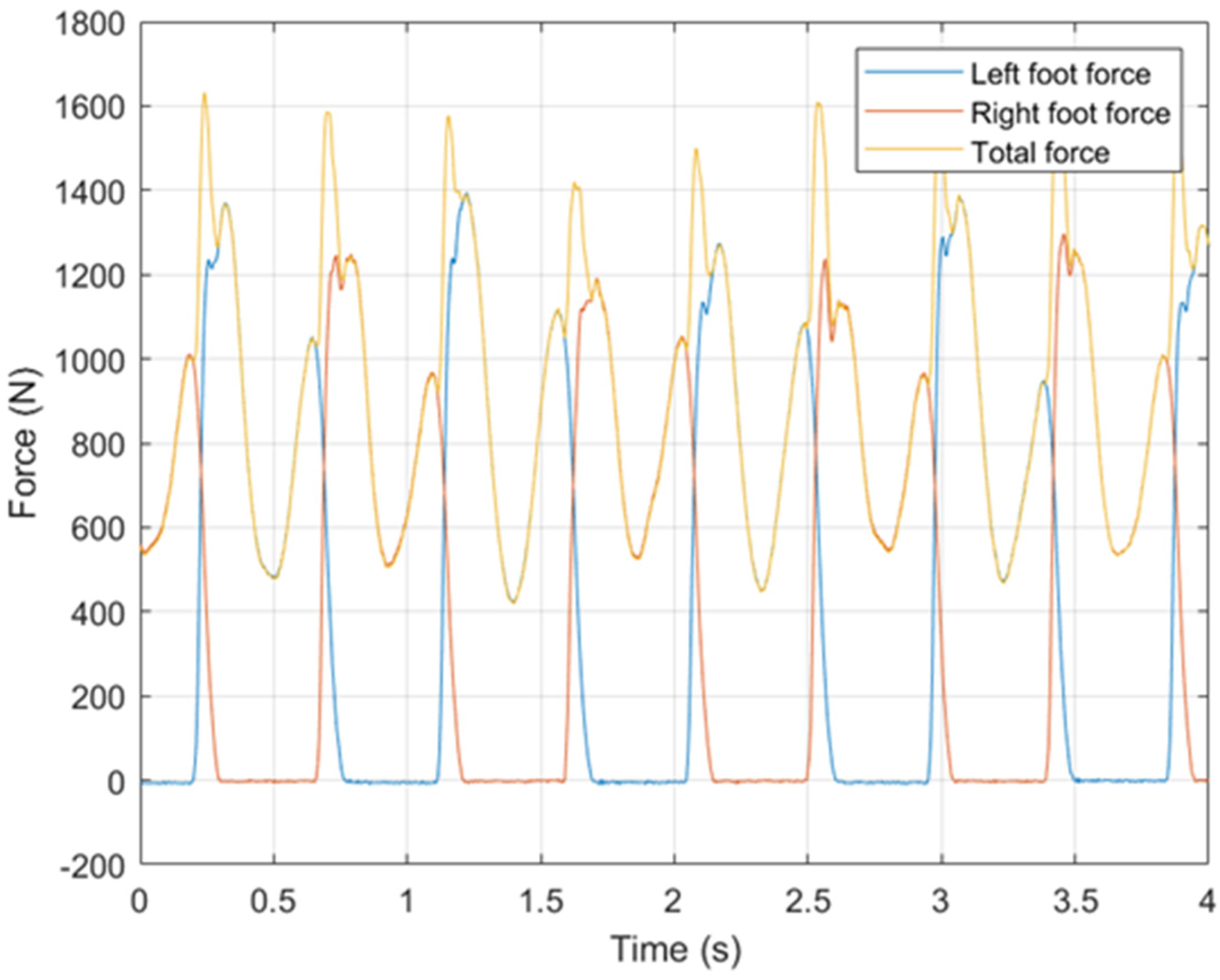
2.1. Experimental Data Collection

Data acquisition was carried by Racic and Brownjohn [29] via a dual belt treadmill [67]. Thus, allowing measurements of the left and the right foot vertical forces to be simultaneously acquired over multiple footsteps (Figure 2). During each walking trial, the speed of rotation of the treadmill belts (referred to as “treadmill speed”) was fixed and controlled by a data acquisition system. Treadmill speeds started at 2 km/h, then at least 64 steps are taken, before a period of rest and then the procedure is repeated at 0.5 km/h faster speed. The procedure was continued until the participant started to jog. The treadmill speed is taken as the average walking speed, whilst small variations may exist due to the participant move up and down the belt, these small variations are considered negligible. The complete description of the experimental setup and test protocol can be found elsewhere [29]. 824 continuous force-time histories generated by 80 volunteers resulted in over ten hours of monitored walking. Due to diverse test subjects and many successive steps within a large population sample, the established database can be used to draw statistical conclusions of the Fourier parameters in Equation (1).

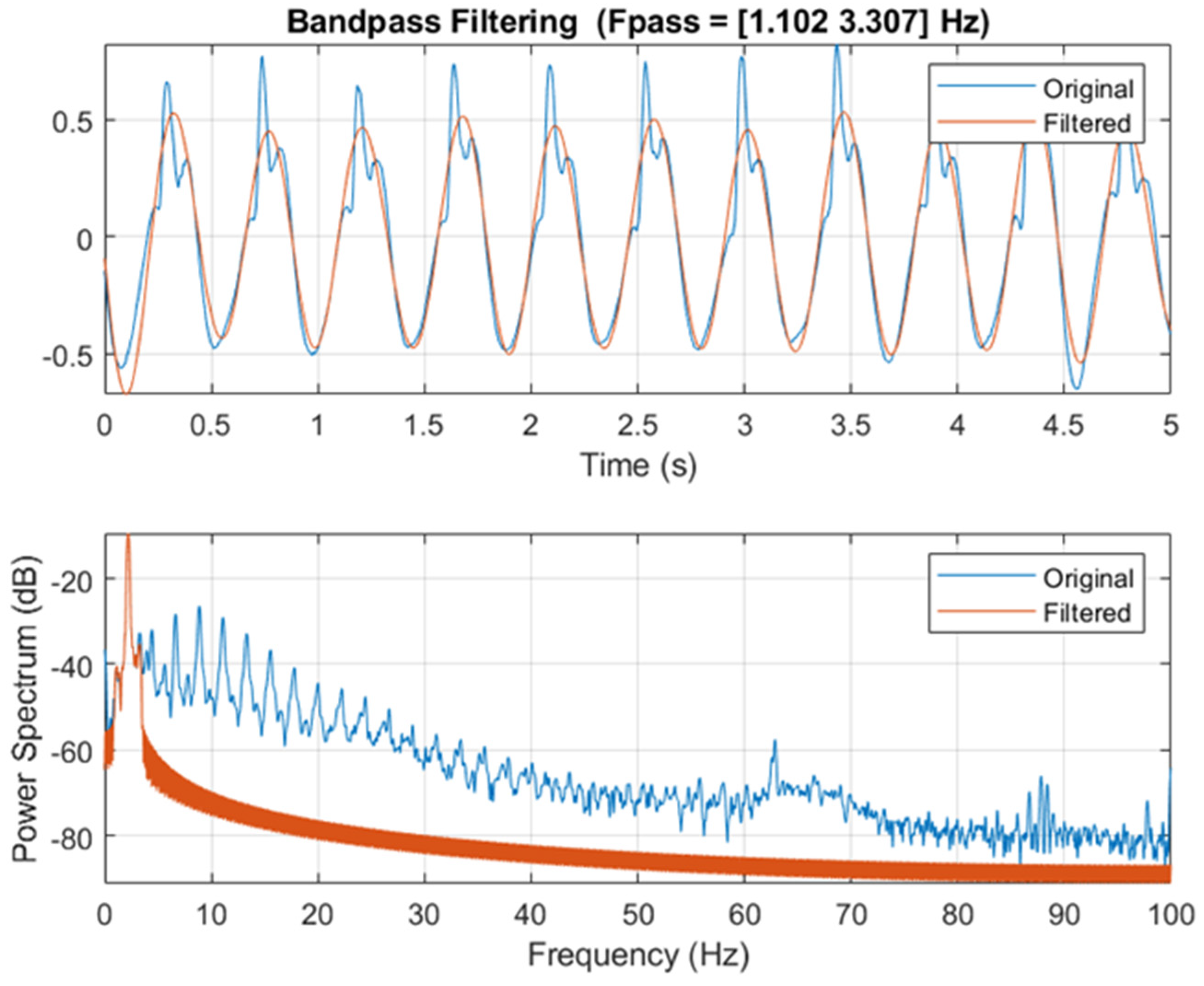
2.2. Data Pre-Processing

The left and the right footfall force-time histories are summed to obtain the total vertical walking force signal (Figure 2). Racic and Brownjohn [29] showed that the DLFs are independent of the participants’ weight W. The body weight representing the static component of the signal, as this component does not affect the dynamic response it is removed from the signal. The resulting dynamic signals were normalised by the body weight leaving a signal as a proportion of bodyweight. Moreover, any force signal with a walking frequency outside the typical range of 1.5–2.5 Hz is discarded as it represents unnaturally quick or slow walking. This selection reduces the content from 824 to 672 measured force-time histories.

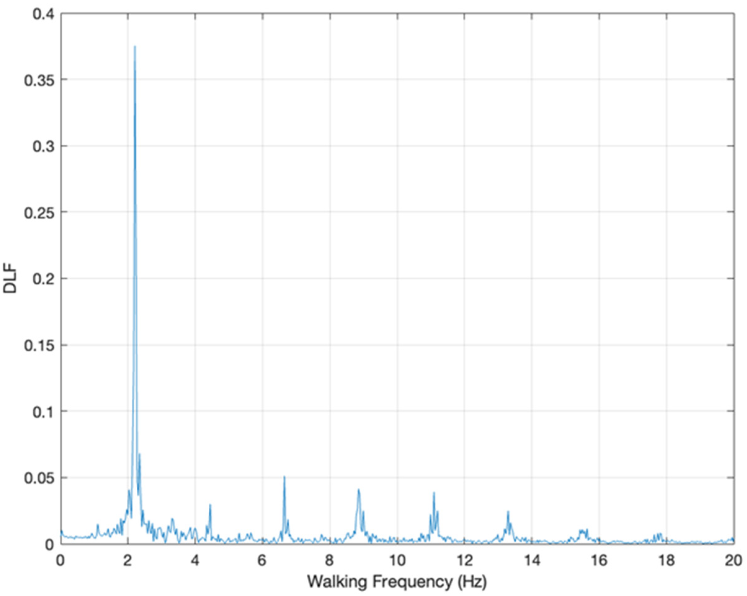
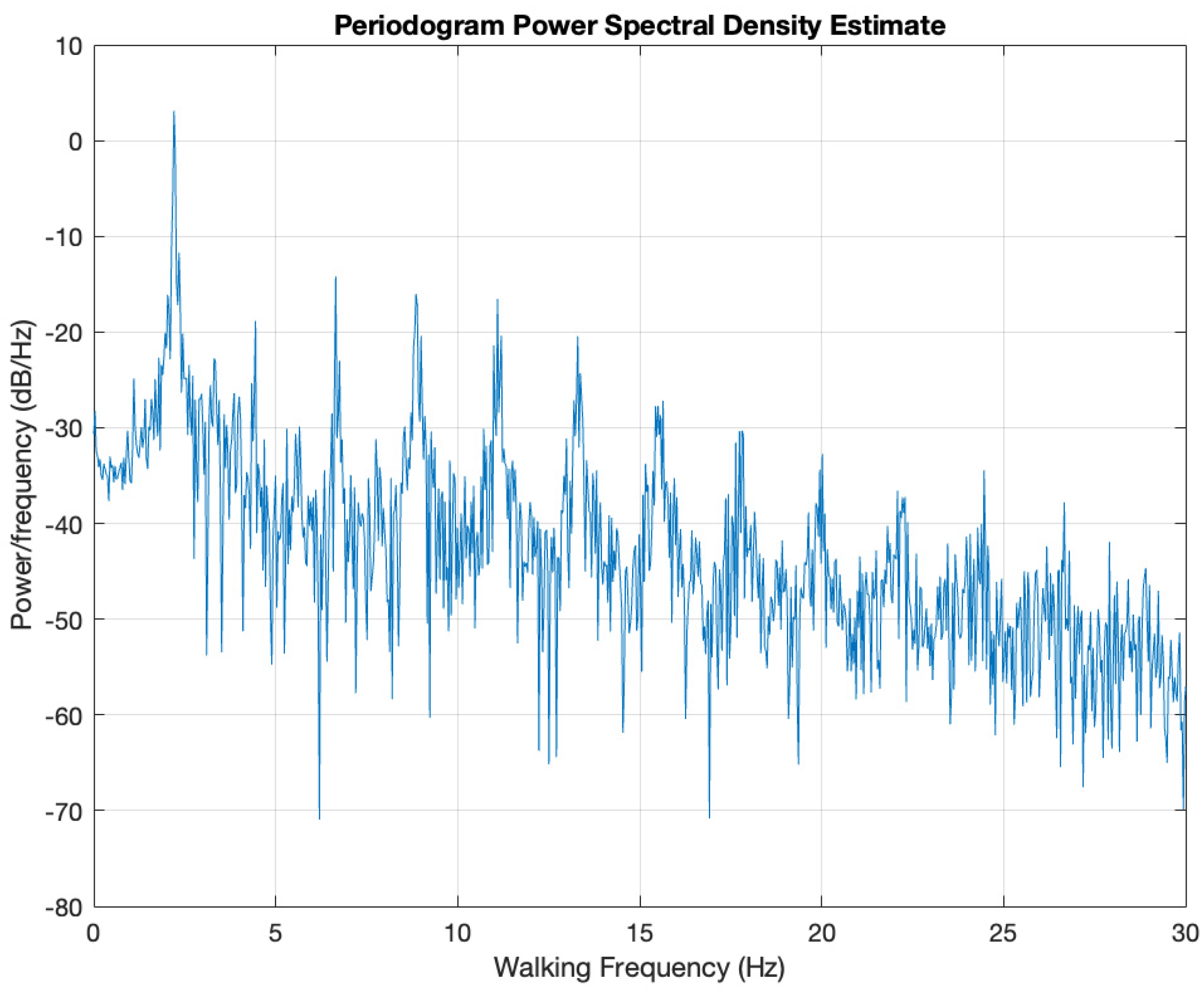
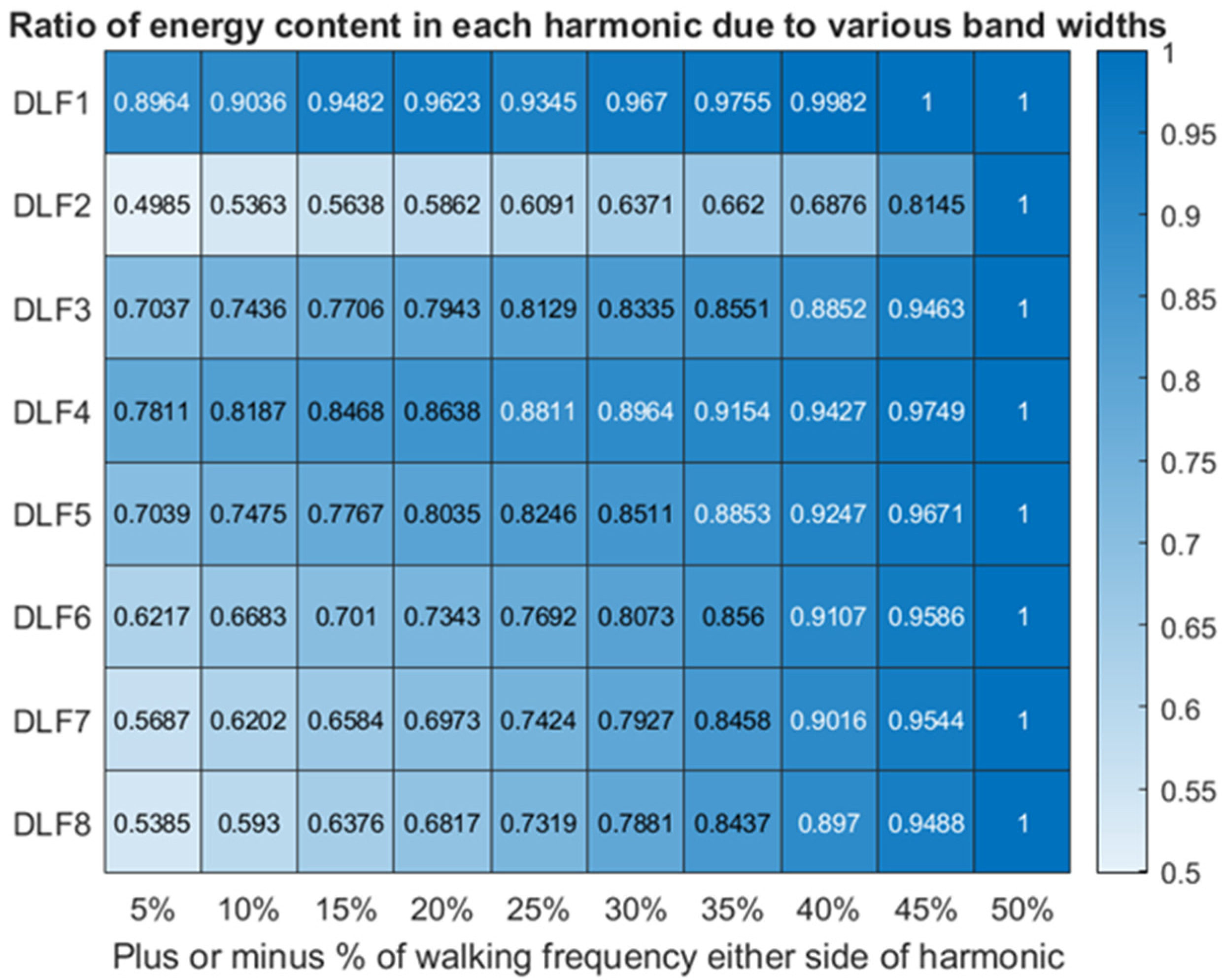
2.3. Extraction of DLFs and Walking Frequencies
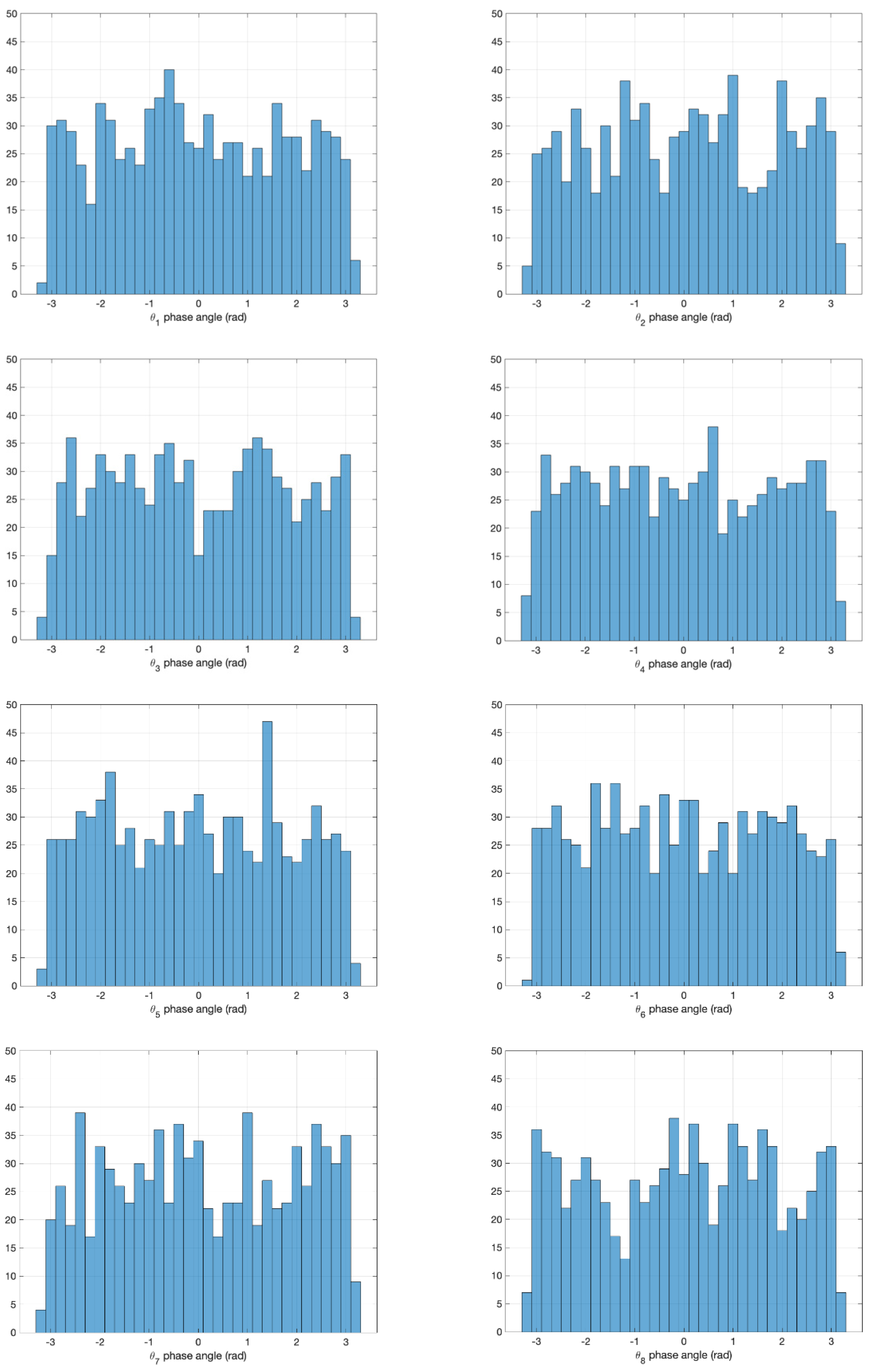
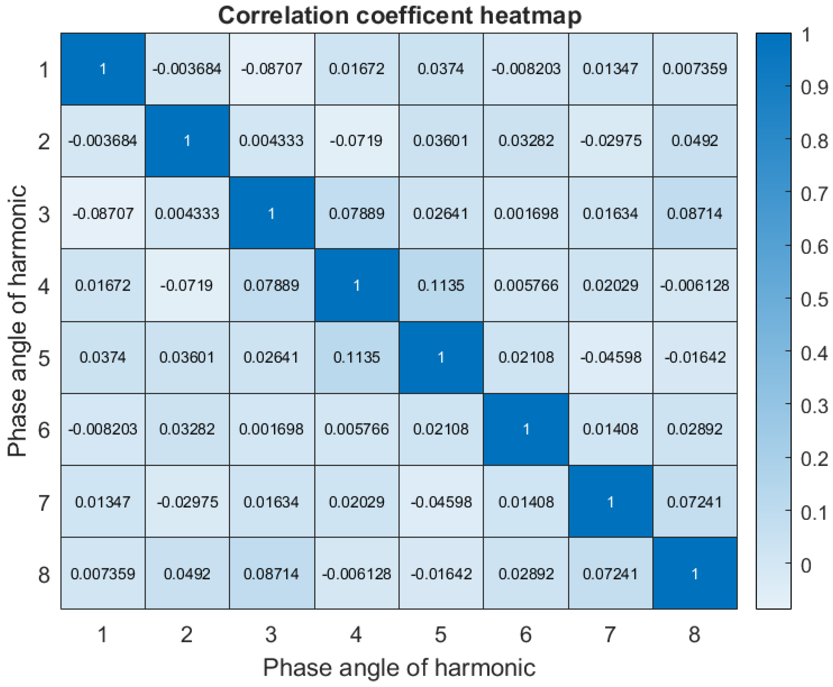
In the frequency domain (Figure 3 and Figure 4), peaks at the integer multiples of the pacing rate are accompanied by energy leaked into their close surrounding frequencies due to the quasi-periodic nature of the force signals as a result of inherent intra-subject variation of walking frequency [27,37]. While the results in Figure 3 and Figure 4 appear continuous, they are discrete and are only used to present a better visualisation of the information. Traditionally the peak value of the integer harmonic is taken as the selected DLF for each harmonic of the walking frequency. Such a constrained methodology negates any information the surrounding narrow-band signal produces [27,28,55]. Whilst the DLF of the peak value provides the majority energy of each harmonic, the surround energy acts to either increase or decrease the relative magnitude of the time signal through slight off frequency forcing functions.
An equivalent DLF value representing the energy around every harmonic (Equation (1)) can therefore be calculated to encompass and combat the downfall of selecting just a peak DLF value. Furthermore, by considering all the energy content of a signal a more representative approximation can be found, not merely a single peak value. Not all harmonics are apparent in Figure 3 due to the small magnitudes they possess at higher frequencies. Therefore, a criterion is needed to assess the necessity of adding additional harmonics of walking. In Figure 4, the power spectral density (PSD) is presented in the log decibel scale. Observations in the log scale allow the higher frequency content to become visible. Figure 4 demonstrates that the values beyond the eighth harmonic appear as not distinguishable from white noise or other low lying forcing frequencies [68].
To determine the equivalent DLF a bandpass filter is used at each harmonic with upper and lower frequency range limits at plus or minus the percentage of the walking frequency. The effect of such a filter is seen in Figure 5. What remains is the filtered signal around the harmonic, considering all frequencies and DLF values around the harmonic. Taking the average of the peaks of the filtered signal reconstructed to the time domain (Figure 5), an estimate of the DLF in each harmonic is made. As the Fourier approximation can be infinitely increased, a cut off harmonic is required to provide an appropriate model. It is postulated based on the authors experience that most pedestrian structures exhibit fundamental modes below 20 Hz. Therefore, due to the insignificant DLF values seen above 20 Hz, coupled with limited structures providing dominate modes of vibrations above 20 Hz. The DLF values observed for the ninth and tenth harmonic range all below 0.005 which accounts for 120 less than the DLF value of the first harmonic. Therefore, it is determined the DLF model will be curtailed at the eighth harmonic.
From visual inspection of Figure 3 and Figure 4, negligible sub-harmonics exist in the data, it is unclear if the values are that of a white noise or very low-lying subharmonics. It can therefore be inferred that the observed gait are close to symmetric, i.e., there was only minor difference between the left and right footfalls. However, it is acknowledged that previous research has shown signs of subharmonics [36,58], that withstand it is not considered in the study.
Figure 6 shows the energy variation in each harmonic when considering various frequency bandwidths around the peak harmonic frequency. Most of the energy is in the first harmonic and is distributed very close to the harmonic peak value. After the first harmonic, the energy content of the signal starts to dissipate over a larger number of frequency. Most of the energy (89.64% in Figure 6) is contained within a bandwidth of 5% of the walking frequency on either side of the first harmonic. This indicates that the first harmonic has a sharp peak consistently across all the results. Thus, the energy content of the signal is seen to act predominantly at the integer. However, other harmonics have larger relative energy spreads. Table 2 presents energy content of each harmonic as a percentage of total energy in entire frequency range.
There is no indication of a correlation between increased energy spread around the harmonic and increase integer harmonic, i.e., the second harmonic of walking has the largest relative energy spread not the eighth, Figure 6. Table 3 presents the average percentage variation in DLF1 with different bandwidth sizes (i.e., frequency filters) around the peak value. It is apparent that the peak picking method produces the lowest DLFs in all scenarios. The value of DLF tends to stabilise after the 10% filter and remains relatively constant throughout baring very rare exceptions. The signals are filtered to ±50% of the walking frequency due to the marginal change in DLF after 10%, and thus choosing 50% ensures all energy influences around a harmonic are considered. As demonstrated in Table 3, filtering the signal around the harmonic of walking produces a DLF value greater than just selecting the peaks. Thus, the energy leakage around the harmonics plays a significant role to provide a more representative DLF value. Taking only the peak would negate, in some cases, 40% of the DLF value due energy leakage and intra-subject variability. Thus, talking a filtered estimate provides an artificial degree of representation of the narrow-band nature of walking.

2.4. Phase Angles

The phase angle associated with each harmonic (Equation (1)) is often assumed to be fixed values [13,22,24,31] or uniformly distributed in the range [−π, π] [29,69]. In the case of resonance by a singular harmonic, the phase angle does not influence the response calculations. However, when the response is composed of multiple modes, phase angles possess fundamental properties to determine if the signals can be constructive or destructive to each other, resulting in an increase or decrease in magnitudes of acceleration. Figure 7 presents the histograms of the phase angles taken at each of the eight walking harmonics derived from the selected 672 force records.
Figure 7 confirms the uniform random nature of the phase angles for each harmonic. Figure 8 further provides evidence of a lack of correlation between each phase angle at each harmonic. The normalised cross-correlation determines the linear correlation of two variables. A score of plus or minus 1 indicates strong positive or negative correlations, whilst a score of 0 indicates no linear relationship of the variables. Therefore, phase angles of each harmonic can be assumed to follow uniform random distribution on [−π, π] interval independent of each other.

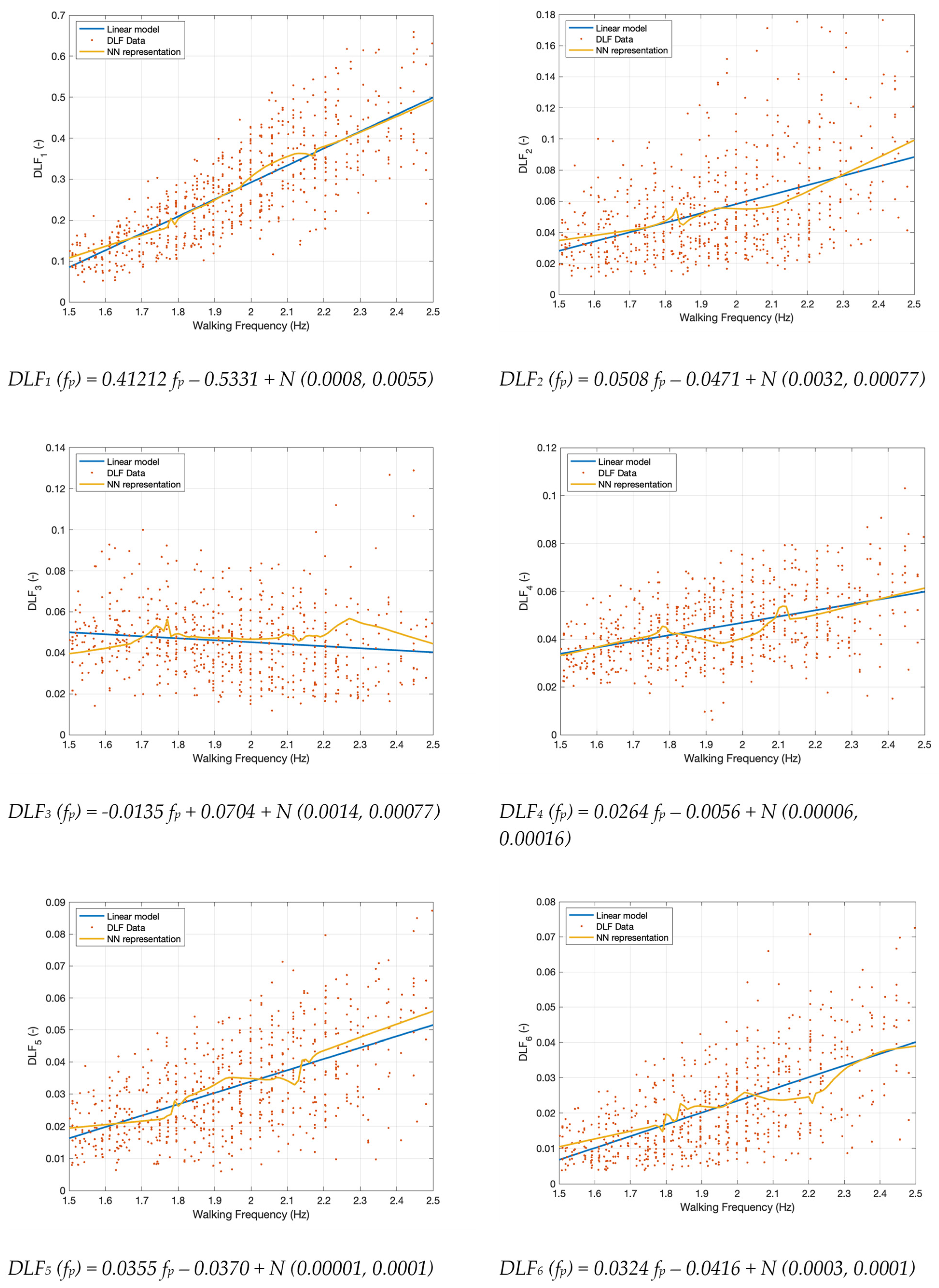
3. Regression Inference of DLFs Given Walking Frequency

There are current DLF models that partially fulfil the requirements of actual statistical inference but lack fundamental inference methodologies [22,24,31,35]. The proceeding subsections demonstrate how statistical inference is performed on the walking force data comparing two statistical approaches: Frequentist (Section 3.1) and Bayesian (Section 3.2).
As with any regression task, the goal is to map independent variables to the output variables whilst minimising the error between prediction and expected value [70], and generalising well to unseen data. In this study, walking frequency is chosen as the singular independent variable for mathematical and physical interpretation convenience. The dependent variables are DLF1 to DLF8. Parametric regression models for the DLFs are in the form [68]:
DLF i = f ( D , ) + ε i , i = 1 , , 8
f ( D , ) is the function that maps the walking frequency (D), using the parameters of the model ( ) to the respective DLFs. Ten different regression models were configured to produce an accurate representation of the walking frequency and DLFs [68] Table 4. The selection of the ten was chosen to provide an exhaustive search for the most accurate model. All regression models are subject to Bayesian hyperparameter optimisation [71] and cross validation to ensure each methodology was optimised to the best extent. To determine the accuracy of each model the Root Mean Squared Error (RMSE) of predictions and true value of DLF is used. A held-out data set is used to provide the score to ensure the model is robust to generalisation and unseen data. The Neural network (NN) provided the lowest RMSE of all the models, second only to linear regression. The usability of the NN model is limited. NN are regarded as black-box optimisers due to the non-convexity of solution space. Linear models have ease of interpretability and familiarity that NN does not. The linear first order polynomial regression is therefore selected as the model of choice. Whilst NN provide the lowest RMSE, the practical use in industry is limited due to the necessity of serving the end user, practicing engineers. Therefore, a useable model that can be easily interpolated needs to be established, that also provides accuracy.
Figure 9 presents the linear polynomial and NN representation of the DLF walking frequency relationships. The NN and linear model appear similar in most instances, with the NN providing local nuances across the walking frequency range. Such artifacts may be representative or an over generalisation of the specific dataset. Thus, the figure provides further evidence for the use of the linear model over the NN. The overgeneralisation of the data is likely a result of DLF values extract, and not the true mechanism of DLF values. As such the linear model will be used as it visually appears to generalise well to the data.

3.1. Frequentist Regression Model

This section provides validation to the underlying assumptions of the linear regression. To ensure the linear regression model is an appropriate estimator of the walking frequency and DLF relationship, the underlying classical assumptions of linear regression must be assessed. The assessment is performed in the context of the ordinary least squares (OLS) and coincidently the Maximum Likelihood Estimation (MLE) approach to parameter estimation first. The classical assumptions are [68]:
  • the regression models are represented through a linear combination of the parameters and error terms,
  • errors are normally distributed,
  • the error term has a condition mean of zero given the data,
  • all independent terms are uncorrelated with the error term,
  • observations of the error term are uncorrelated and non-auto-regressive,
  • errors have constant variance, homoscedasticity.
As seen in Figure 9, the data appears approximately linear for DLF1–DLF8 with respect to the walking frequency. The general parametric form of the linear regression can be rewritten to describe the errors:
ε i = DLF i D T   , i = 1 , , 8
For all DLFs, the normal distribution of errors is assessed through the one-sample Kolmogorov–Smirnov test using the standard normal curve as a reference, i.e., εi~N (0,1) [62]. The null hypothesis statement is that the residuals are drawn from a standard normal distribution. The alternative hypothesis is that the error does not come from the distribution at a significance level p = 5% [72]. First, a pre-processing step is performed on the raw residuals of each DLF. The Z score of each residual is taken to normalise the data into the same length scale as the standard distribution:
    Z = ε μ ¯   σ ¯  
As the actual population mean and standard deviation are unknown, the sample mean μ ¯   and standard deviation σ ¯   are used instead. Four out of eight DLF errors are normally distributed (DLF2, DLF3, DLF7, DLF8) with the remaining errors becoming normally distributed if the significance level is adjusted to 10%. Therefore, for such a random process such as walking, a linear model provides a good approximation of the data. The third assumption of the OLS is inspected through the mean values of the error for each of the harmonics: 0.0008, 0.0032, 0.0014, 0.00006, 0.0001, 0.0004, 0.0008 and 0.0011, respectively. Whilst the values of the mean are not exactly zero the magnitude of the mean is negligible compared to the magnitude of the DLFs they represent. Therefore, the residuals can be assumed to be sampled from a zero mean Gaussian function.
The assumption of homoscedasticity of the data is central to linear regression models and entails the errors having constant variance, being independent of the input variable and non-autoregressive [73]. To determine if the data is autoregressive and conditional heteroscedastic the Engle test [74] is performed. The null hypothesis that the residual errors come from a heteroscedastic series is confirmed. Therefore, the data possess a changing variance of error depending on the input.
The consequence of heteroscedasticity means the OLS estimator is not the best linear unbiased estimator and the variance of the errors is not the lowest of all the unbiased estimators. The presence of heteroscedasticity does not cause the parameters but the error variance to be biased. Weight least square regressions are employed to address heteroscedasticity [75]. Each observation is weighted using a diagonalised matrix to bias results closer to the mean and penalise result far from the mean, before the normal equation or maximum likelihood estimation is performed [75].
Figure 9 presents the weighted linear regression through the lens of the Frequentist statistics, where each DLF is mapped to the various integer walking harmonics from 1 to 8 along with the associated equations for each DLF. To obtain the DLF at each harmonic integer, the walking frequency is inputted into the corresponding equations given in Figure 9. If a result other than the mean value of the DLF is desired, the distribution of each error of the DLF is also found in Figure 9. The error can then be sampled using an appropriate normal distribution sampler with the corresponding mean and standard deviation values given in Figure 9. Furthermore, if a desired level of probability of exceedance is required, the appropriate z look up tables can be used based on the mean, standard deviation and confidence interval.

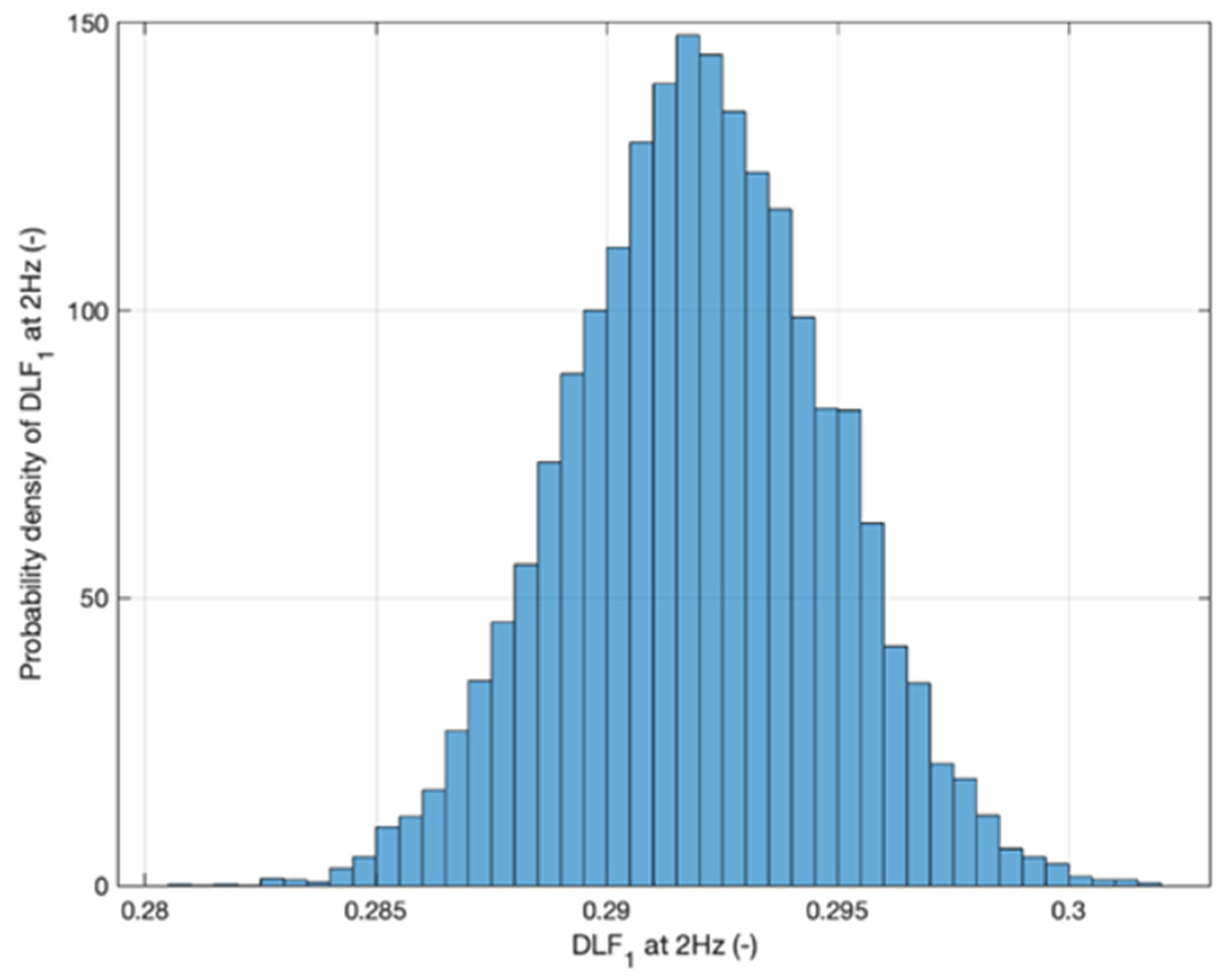
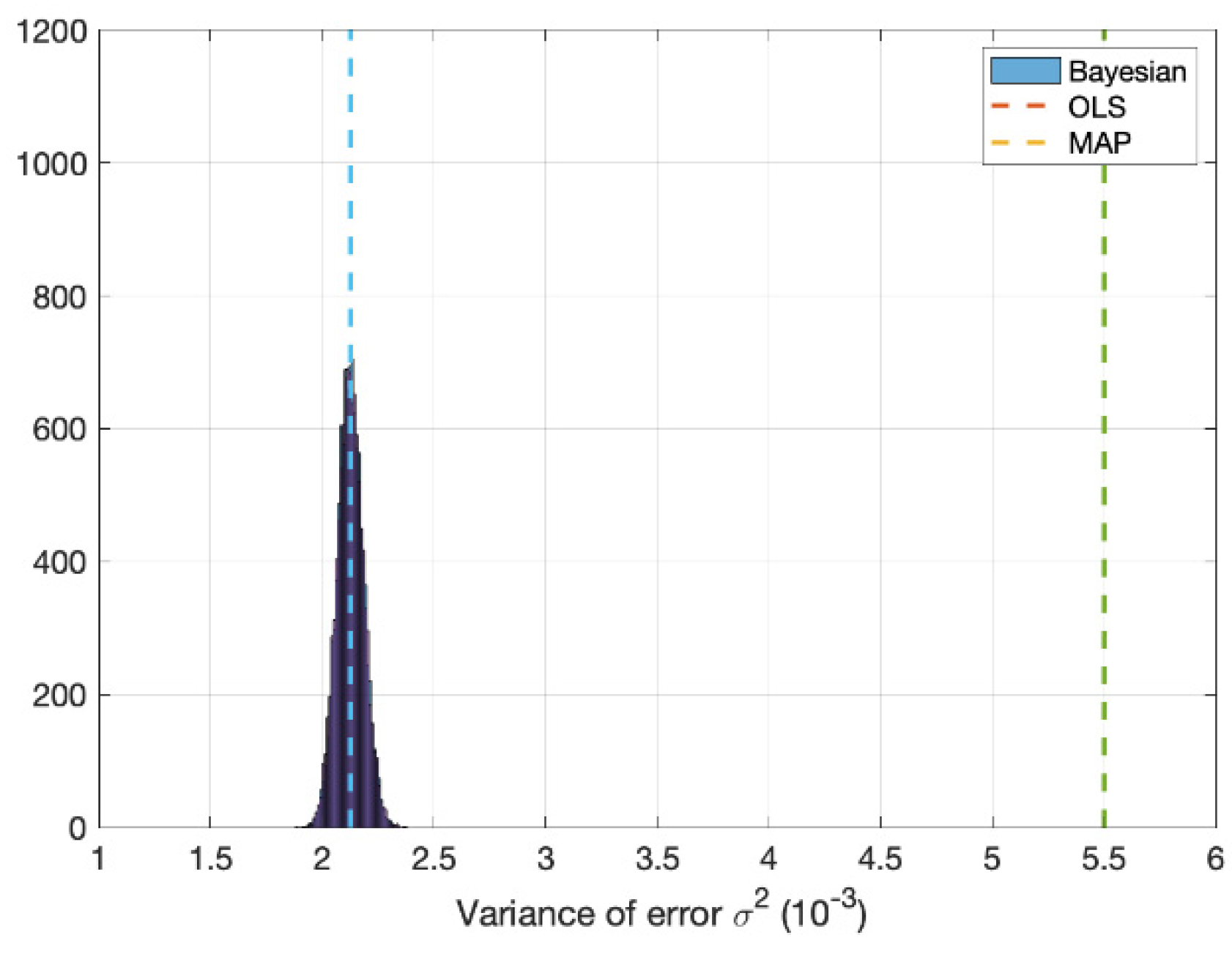
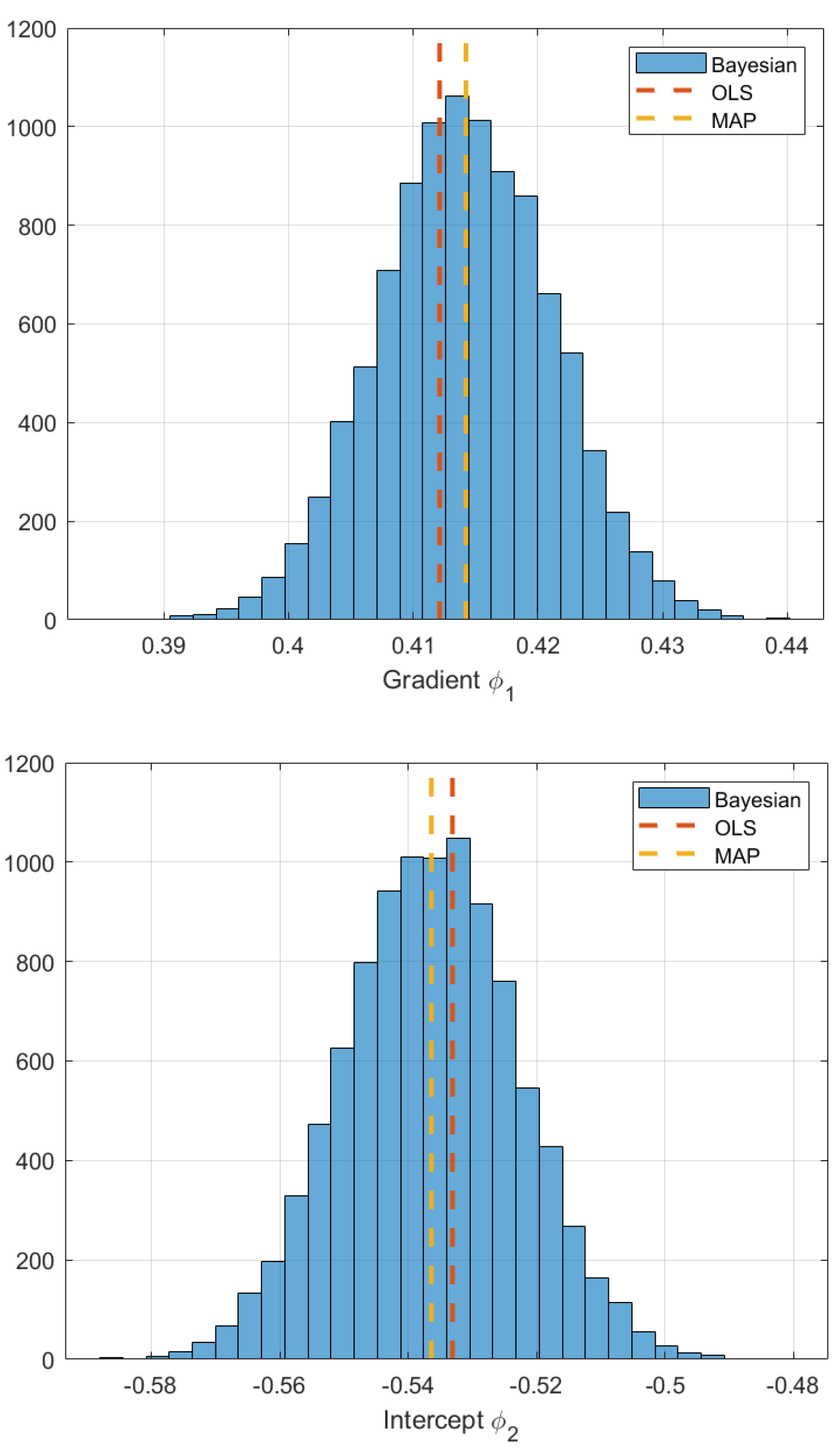
3.2. Bayesian Linear Regression Model

In Bayesian inference, the parameter value is defined through a probability distribution, even though the parameter’s actual value is fixed and static [76]. Moreover, Bayesian inference provides a framework to interpolate the parameter given the prior belief and knowledge of the parameters. As more data becomes available, the variance over the parameter estimation decreases and alters the prior belief. Thus, the posterior distribution is gained via [70]:
P ( | D ) = P ( D | ) P ( ) P ( D )
where P ( ) is the prior probability estimate of the model parameters , before any of the data D is observed. P(D| ) is the likelihood function. It represents the likelihood of the data given the parameter. Finally, P(D) is the marginal likelihood and is the distribution of the observed data marginalised over the parameters. This denominator ensures the posterior distribution integrand integrates to 1, giving a complete probability distribution.
The prior belief of the parameters P ( ) must be first established. This can be done in two manners: either using an informative or noninformative prior [67]. The latter is considered uniform over the entire parameter space and provides no insight into the current problem. The informative prior assigns a staked probability to the parameter space in the region of belief. As previous studies of DLFs have modelled the parameters linearly [13,22,24,31], and the Frequentist approach has been analysed in Section 3.1, the solution space can be assigned an informative probability distribution. The Bayesian model will use conjugate pairs for computational simplicity, thus allowing the posterior distribution to be analytically tractable and of the same analytical form as the prior. The closed-form nature of the conjugate prior speeds up calculation and does not require numerical integration [77]. Assuming that each value of DLF is extracted independently from a normal multivariant distribution the likelihood function of the DLF given the input and the model parameters can be taken as:
P ( D | ) = P ( DLF | w f , 1 , 2 , σ 2 ) = n = 1 N N ( DLF n | w f n , 1 , 2 , σ 2 )  
where 1 , 2 , σ 2 are the gradient, intercept terms and variance of the gaussian noise, whilst subscript n is the nth data point of the set of DLF and walking frequency values. Thus, the observed values of the DLF given the input values of walking frequency dictate the evidence of model parameters. Therefore, the maximisation of the likelihood function corresponds to the maximum likelihood estimator from which the OLS estimation can be derived. The derivation of this can be seen elsewhere [68]. Hence, similarities of the Bayesian framework and frequentist framework can be seen. However, in the frequentist case it used to derive a singular value of estimates.
^ M L E ( D ) = a r g max P ( D | )
The Bayesian framework is concerned with the distribution P ( | D )   thus providing the uncertainty of the parameters given the data, the posterior distribution. The exact formulation of the likelihood function is dependent on the observed data.
A similar first order polynomial regression model is used to assign the corresponding DLF values with the walking frequency. Therefore, probability distribution must be assigned to the intercept, gradient and standard deviation of the error. In the Bayesian framework the distribution of the error is described through zero mean gaussian process with unknown standard deviation distribution, typically described through a probability density function that is strictly positive. The gamma family of functions is used in the present study to model the prior and posterior distribution of the parameters, which includes the exponential family of functions such as the Gaussian distribution and student t distributions. The gaussian distribution is used to model the prior of the intercept and gradient term of the linear model, whilst the gamma function itself will be used for the error variance due to the variance being a non-negative value. The gamma function is parametrised by the shape and rate variables, (α, β). More detailed information on obtaining the posterior distribution using conjugate priors can be found elsewhere [70].
As the posterior distribution is in an analytically tractable form, the posterior can be readily sampled and the use of simulated methods such as Markov Chain Monte Carlo methods are not needed. An example of the posterior distribution of DLF1 for a 2 Hz walking is seen in Figure 10. Similar to the MLE, a singular value of most likely parameters, the maximum a posteriori (MAP) estimate can be used to compare the most probable values of the MLE and Bayesian framework. The MAP of the parameters ( ^ M A P ) is given as the maximisation of the likelihood and prior functions [70]:
^ M A P ( D ) = a r g max P ( D | ) P ( )
As the marginal likelihood is always positive, it has no bearing or dependency on the parameter set . Therefore, it can be ignored in the optimisation of obtaining the MAP. The marginal likelihood is achieved through integrating out the parameters   of the likelihood and prior function. Such an integration is only known for a small number of conjugate prior functions, therefore numerical integration is often required. This presents further complications due to increased computation time when the number of parameters are numerous. Therefore, when non-standard priors are assumed the proportional relationship of the likelihood and the prior to the posterior distribution is often found instead. From Equation (6) it can be seen than the MAP and MLE will coincide with their estimations when a non-informative prior is used. Therefore, the a priori estimation provides meaningful insight and guidance to the optimisation of the parameter estimates.
In all but the variance of the error, the MAP and MLE estimator coincide well. However, as seen in Figure 11, the error variance is lower compared to the OLS estimator. As previously discussed in Section 3.1, the data is heteroscedastic. Therefore, the estimate of the error will be biased. In the Frequentist approach, the mean is marginally nonzero, resulting in a shift of estimation of the mean value. Hence, the variation of the error will subsequently increase. In the Bayesian framework, the mean is assumed precisely zero and the error variance is inferred, resulting in a slight shift in results due to the data not having a zero mean.
The prior of all the DLFs will be taken as a gaussian distribution with means taken as the value of the Frequentist approach and covariance matrix taken as the two-dimensional identity matrix multiplied by 0.1. The resulting 672 degree of freedom student t posterior mean, covariance and variance of the error are presented in Table 5. To sample the Bayesian model for the corresponding DLF’s, first the appropriate walking frequency must be selected. Then, given the multivariable student t distributions of Table 5, successive sample can be drawn of the gradient, intercept and standard deviation of the error, thus giving a posterior distribution of the output DLF values marginalised over the previous parameters, such that the P ( 2 | 1 ) ,   etc . , is satisfied. Figure 10 provides the posterior distribution of DLF1 when the walking frequency is selected at 2 Hz. Such a distribution represents the probability density of DLF1 given the walking frequency.

4. Discussion

This section presents a retrospection of the outputs from the regression inference from the previous section. The MLE and MAP estimation outputs are compared in their likeness and justification in Section 4.1, while the Frequentist and Bayesian approaches pertinent to the present study are compared to DLF models from the past studies in Section 4.2.

4.1. Bayesian vs. Frequentist Approach to Fixed Parameter Values

The OLS and MAP values of the model parameters are shown comparatively in Table 5. The values coincide well, with only a few varying by 10−4 in most scenarios. Such a variation is negligible in comparison to the values they represent and can therefore be considered approximately similar. When sampling the Bayesian approach 100 times and comparing it to the Frequentist model of DLF1 (Figure 12), the model estimates align and represent the data similarly. The OLS and Bayesian estimate converge when large amounts of data are available. Taking the log of Equation (8) does not affect the properties of the maximisation but allows the separation of the terms, as the log function is monotonic the maximisation of occurs at the same location as the non-log function. The MLE arises plus a regularisation term, log ( P ( ) ) (log of the prior distribution). Thus, the OLS and MAP will eventually coincide when large amounts of data are present, and the prior is not significantly biased. Moreover, the Bayesian MAP will become a more data centric estimation of the parameter rather than the prior [70].
^ M A P ( D ) = a r g max θ [ log ( P ( D | ) ) + log ( P ( ) ) ]
The only inconsistency of both methodologies is that of variance of the error, as illustrated in Figure 13. In DLF1, the variance of the error of the Bayesian model is estimated to be about half as much as the Frequentist approach. This result arises due to the combination of a poor prior estimate and the variance of the models are heteroskedastic. As seen from Figure 11, Figure 12 and Figure 13 the Frequentist and Bayesian approaches are approximately identical. The preferred use of one model over the other is therefore down to the discretion of the user and their philosophical view of statistics.

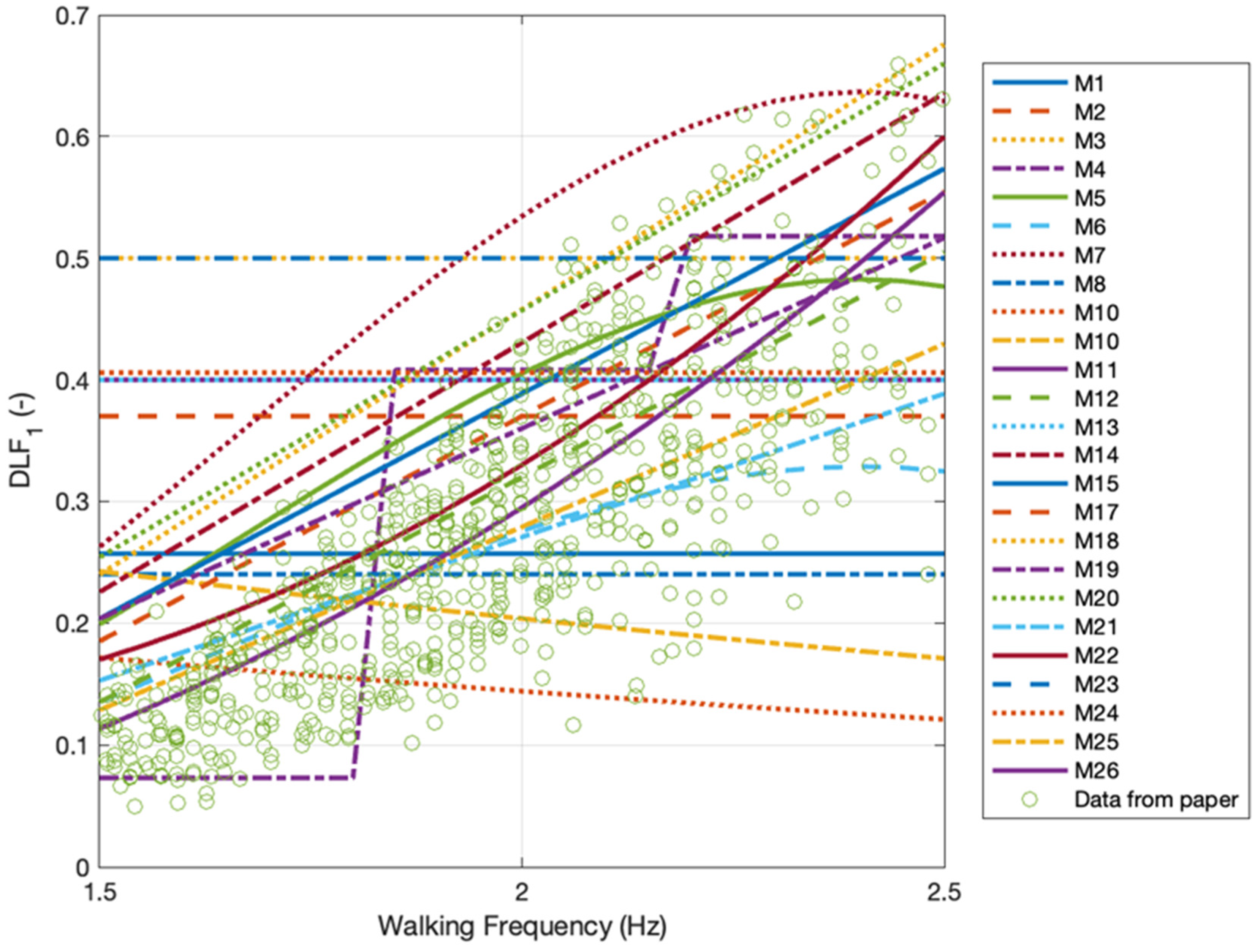
4.2. Comparison of Proposed Models against the Current State of the Art Models

The formulated models are compared in Figure 14 to the existing Fourier series models [13,31,35,42,59,61] that are deemed state of the art [37,78]. Table 6 present the limiting walking frequency ranges of each Fourier-based model. As seen, numerous industrial vertical load models provide a limited range of feasible walking frequencies. However, researchers have continually provided evidence that demonstrates walking occurs through a normal distribution centred at 1.8–2 Hz and can exceed walking frequencies of 1–3 Hz [44,79,80]. Therefore, limiting the walking frequency of a model devalues structure with natural frequencies just out of the range. It is seen in Figure 14 that the greatest DLF values are seen at 2.5 Hz, thus the models of AISC Design Guide 11 [22], ISO 10137 [13], SCI P354 [31] and SETRA [25] all do not consider the highest values of DLF. The limitation of international guidance on walking frequency further causes misinformation of vertical walking forces, through perceiving that walking frequencies out of the ranges as not important. This may result in higher order harmonics of a lesser walking frequency being used to match a resonant mode instead of a higher frequency first order mode. Furthermore, the curtailment of walking frequency is concerning since the data used to model the DLF’s of the limited model is largely from Kerr [35], where walking frequencies from 1–3 Hz are monitored and measured. Therefore, the limited models purposely reduce the results through choice and not through lack of data.
The formulated model of the paper result in a lower magnitude of DLFs than all the other models, barring that of DLF2 above 4.8 Hz. Varela et al. [61] provides a close representation of the first integer of walking, the model closely resembles that of the proposed model for the first integer. The results of Varela et al. [61] start to diverge in the successive integers and only represents a limit number of harmonics. Varela et al. [61] model produces higher DLF values for the third and fourth harmonic than the presented data. Varela et al. [61] appears to only model the extreme high value of the data at high harmonics resulting in larger than required DLF values. Varela et al. [61] suggests DLF values to be elevated at lower and higher walking frequencies compared to the presented model in the first harmonic, however the datapoints in paper do not suggest as such with the data more accurately represented through a 1st order linear regression. Section 3 explores the idea of higher order linear regressions but all produce worse RMSE values. As walking frequencies are normally distributed less information is seen at the extreme high and low walking frequencies. Coupled with the heteroscedastic nature of walking the precise nature of the DLF at higher walking frequencies is not known with much confidence. AISC DG 11 [22] model provides a vast oversimplification and overestimate of the first, second and third harmonic and represents a poor estimation of the dataset. At higher harmonics of walking, DLF values of industry models provide a similar magnitude of responses to the data points. This is a result of the relatively low values of the DLF, however significant percentage error differences are seen. Figure 15 shows a historical trend of walking forces having higher DLFs. This could be speculatively attributed to several issues, such as “white coat syndrome” making people walk unnaturally, the short lengths of older force plates making participants target footfalls on the force plates thus creating unnatural force waveforms, improper modelling due to heteroscedastic data, improper inference or lack of error estimation, test subject population differences, bias population or bias results due to a low number of data points recorded by force plates, the bias of results due to replication of force-time histories to produce higher resolution results, etc. Previous models have mistreated statistical information of the data resulting in some misguidance of the range of DLF values [13,31,42,59].
The results of Figure 15 indicate that even when differing modelling methodologies are used, similar results are found for models derived from treadmill data. All the results coincide and produce lower magnitudes of DLF1 compared to that of the force plate measurements (Figure 15). Noting that Brownjohn et al. [55] data is limited to three subjects. Hence, the results are not as statistically comparable to the present study. The results’ consensus indicates that the presented models align well with historic treadmill data for similarly obtained results. As such the multiple step measurement of vertical walking forces allows for a more accurate representation of the mean properties of walking compared to their single step counterparts.
In the case of Kerr’s models [35], the equation of DLF for 5% error model appears to fit the mean value of the proposed DLF model rather than the 5% error of the data. This again shows the historically high DLFs derived from force plate data compared to the current treadmill data [29] (Figure 15a,d). In the case of the 95% model, the equation appears to not represent the shape of the data. As seen in Figure 15 the cubic nature of the data misrepresents the approximately linear data. Along with the improper use of statistics, it is clear the DLF values are misrepresented through their statistics. However, it is noted that the population samples are both different in size and people. Therefore, some variation may be a result in fundamentally different walking attributes.
Due to the significant variance and heteroscedasticity, the error in the linear models of the present models produces negative values of DLFs at low values of walking frequency for the 5% error model (Figure 15a). This is not feasible and shows where the proposed model starts to break down. Due to the data dependant variance, the overall estimation of the error is more extensive in regions of the model than is presented in the data. This means the model is not the best estimate for all the tasks but provides a more accurate expectation than previous models. Furthermore, a simplistic model such as a linear regression based on walking frequency is an oversimplification of the complexity of walking.
Nguyen’s [59] 90% and 95% confidence interval (Nguyen refers to them as fractal values) validates the results of the 90% and 95% of the Frequentist and Bayesian models presented in the paper (Figure 15c,d). The DLF values are within the same range as the models presented in the paper for the 90% and 95% error estimation. However, Nguyen [59] used only single footfall measurements and temporally shifted the wavelet to provide a complete force-time history. This biased the results due to a single footstep measurement representing the entire force. The dataset of the present study far outweighs any other study of its kind and is therefore used a baseline of reference in comparing all other models and datasets.
The historic over estimation of vertical walking load models further suggesting either the data is statistically different from the presented study, or the data acquisition and modelling methodology resulted in significant difference. Figure 16 shows the variation of DLF1 using the filtered method in the paper compared to peak picking. As shown in Figure 16, using the peak picking method on the data results in lower magnitudes of DLF compared to the filtered method presented. Therefore, compared to previous models’ peak picking, the resultant DLFs would produce a force time history of even lower magnitude than that of the proposed model in the paper. Hence, it can be seen that the variation of DLFs with respect to previous models is a result of the quality of the data and the inclusion of the intra-subject variation of the data. The intra-subject variation of data therefore plays a crucial role in selecting an appropriate DLF value.
The concept of confidence, credible intervals, and error have been used interchangeably throughout civil engineering literature despite their different meanings. Confidence intervals are attributed to Frequentist statistics. A Frequentist can therefore only state if the parameter is or is not in the intervals over similarly drawn samples some proportion of the time [67]. In the Bayesian context the credible interval is found from the posterior distribution [64]. The highest density interval (HDI) is then used to establish the credible interval. HDI is defined as the region covering the sample space for a given probability that has the smallest possible interval over the sample space. The reader is guided to Schoot et al. [77] for broader guidance on Bayesian statistic and modelling.
In statistical inference of a regression model, it is necessary to estimate the error in the model. Such an error is not from the incapability of the model, but errors arising from unobservable differences in the data. Therefore, the error of any model’s output is independent of the model parameters themselves. As such the inclusion of any error estimation will merely linearly increase or decrease the value of the output and does not affect the actual parameter values. Examples of misuse of the error and confidence bands are seen in [24,35]. Both models use confidence intervals over parameters, not the error estimation of DLF values. There is not a correct statement for CCIP (cement and concrete industry publication) load model [24]. The document states that the equation presents DLF values for 25% chance of exceeding. However, compared to their mean value, all parameters of the equation change. This therefore indicates that the statement refers to the likelihood of the parameters and not the likelihood of the DLFs. For Kerr’s model [35], the valid statement is “the confidence interval would include the true parameters of equation for 95% of similarly drawn intervals “rather than the current hypothesis that states the 95% confidence interval of the DLF is in the range. In both cases, [24,35], the statements do not provide an estimation of the likely DLF values but the parameters describing the DLF relationship. This is further evidenced in Table 1 when all values of the equations change, thus suggesting the erroneous statement and or that the data is heteroscedastic and, like the paper, the variance of the error changes with the input. However, no such statement is made in the referenced texts.
The models presented in the paper provides the most accurate representation of the data across all harmonics. Thus, the presented models will provide more accurate response than any of the counterparts when a multimodal response is calculated. Often a singular mode dominates the response and as such the multimodal response of a structure is not considered. However, for complex structures often multiple modes exist near one and other and have multiple dominate modes. Therefore, using current industry models, the current poor estimation will be exaggerated by the lack of accuracy of higher order harmonics of the DLF. As seen in Figure 9 and Figure 14 the presented models provided a more accurate representation of the DLF relationship than any other model.

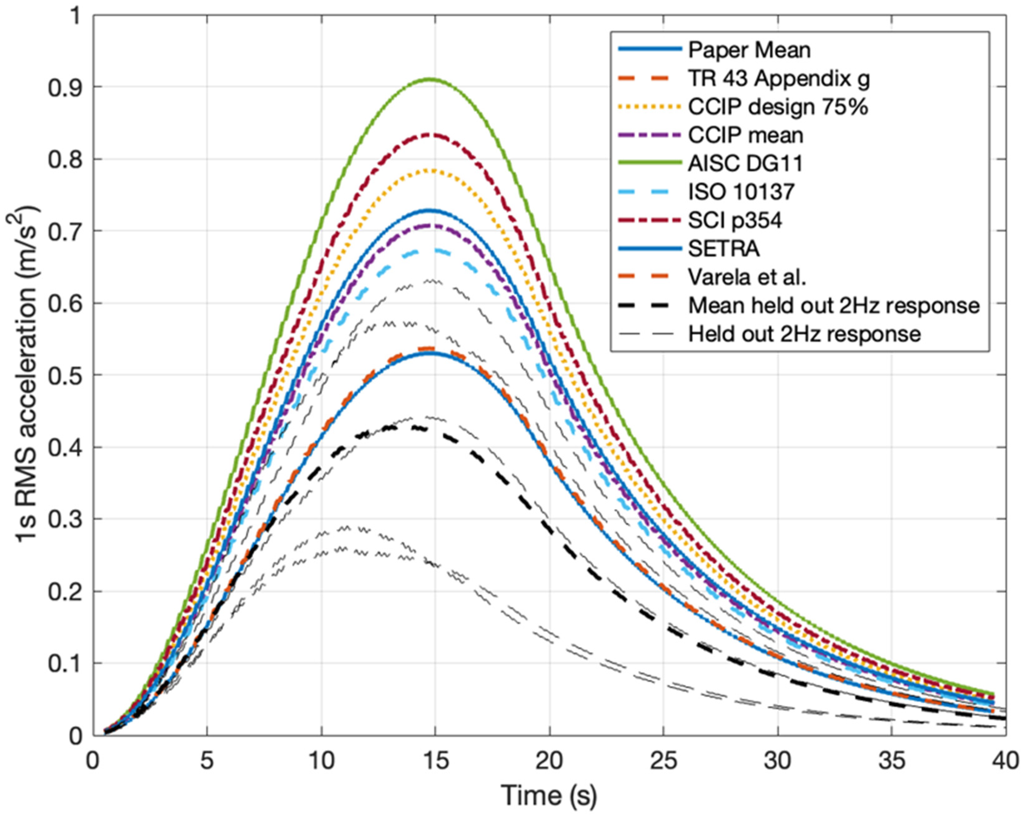
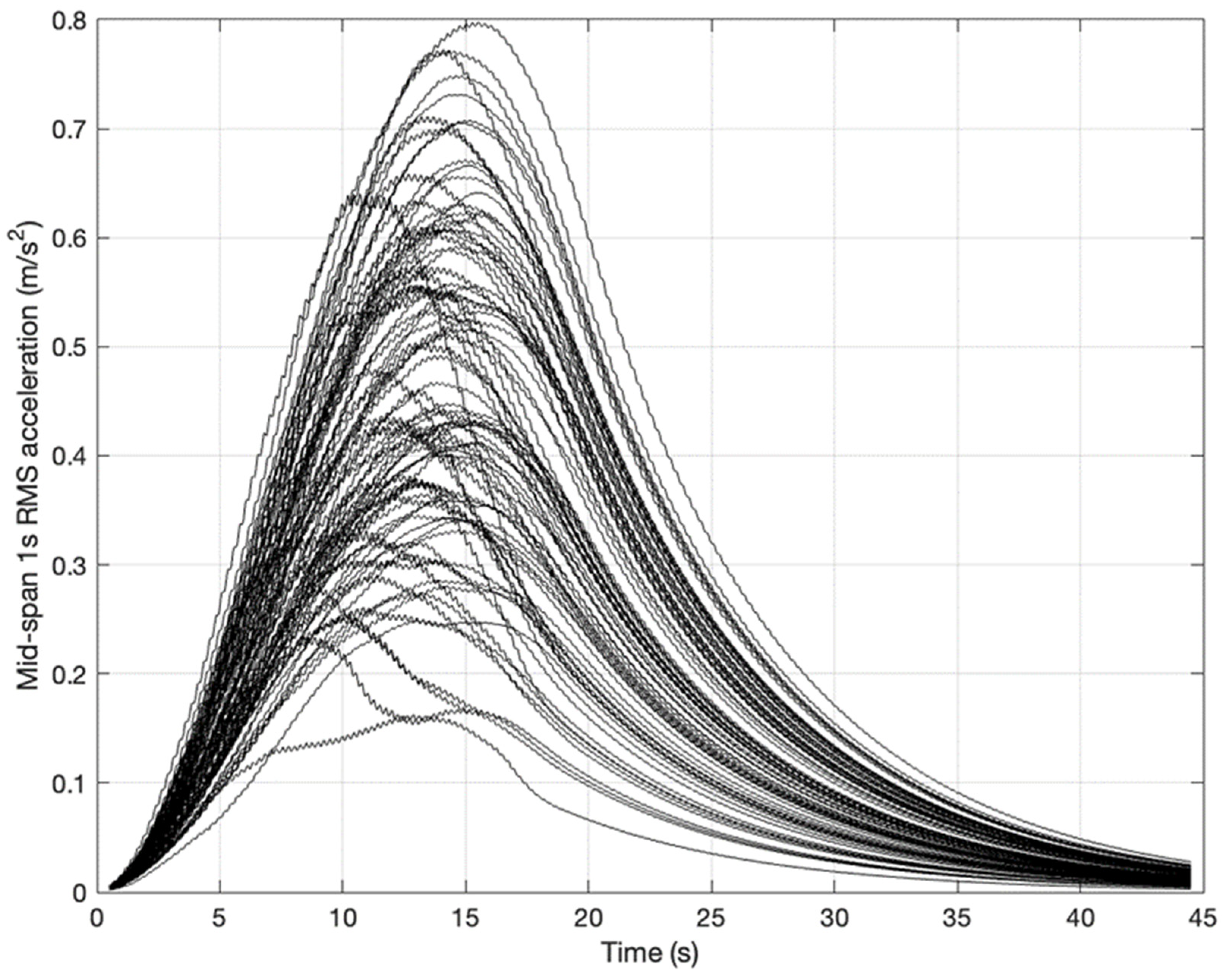
4.3. Comparison of Acceleration Response

To provide a comparison of the proposed model to current industry used models, the acceleration response of a held-out number of continuous force time histories are compared to the proposed models and industry used load models. A fictious single degree of freedom simply supported structure is used as a base structure. The modal damping is taken as 1%, modal mass equal to 10,000 kg, natural frequency of 2 Hz and total span of 30 m. The values chosen are used to represent that of current pedestrian footbridges and values presented in guidance [25,31,66] and to ensure all models are within their usable range. The span was chosen to allow a resonant build-up of accelerations and the natural frequency was chosen to match the mode of walking frequencies [44]. The 1 s root mean squared (1 s RMS) acceleration is use as the metric of choice due to its popularity in use throughout VSAs, and it also acts to smooth out singular peaks in acceleration from stochastic processes. The first mode of vibration is only considered due to the significant DLF magnitude compared to successive modes. No human structure interaction forces are considered hence only the rigid force effects on the structure are considered. However, it is noted that significant biodynamical effects will occur when a pedestrian walks across a real structure [48,61]. These human structure interaction effects will result in different gait and force variations of the individual [82,83,84]. However, such additions are beyond the scope of the paper.
The models compared are: SCI P354 [31], CCIP Design and mean values [24], AISC design guide 11 (2016) [22], ISO 10137 [13], Setra [25], Technical report 43 Appendix G [23], Varela et al. [61]. The presented models mean values are compared against a held out set of five continuous force time histories at 2 Hz walking from the dataset of Racic and Brownjohn [29]. The signals will all be multiplied by a pedestrian weight of 750 N to provide a comparative example.
Figure 17 provides the mid-span 1 s RMS acceleration comparison. As seen the mean values of the model presented in the paper best represent that of continues walking load models along with the model of Varela et al. [61]. The likeness in Varela et al. [61] is anticipated due to the closeness in DLF1 relationship the paper and Varela et al. [61] poses at 2 Hz. Current industry used load models [13,23,24,25,31] provide consistently higher predictions. With some providing close to two times the expected 1 s RMS acceleration. It becomes clear from the small sample of held out data that current industry used models do not predict the correct mean walking force function. Deviations in all the results from the measured signal may be a result of such a small sample size of held out data. However, due to the magnitude of difference it is anticipated that the data from previous DLF models are not representative of real walking forces.
Whilst Figure 17 only provides a limited cross section of each models response to an arbitrary structure, it becomes evident from the combination of Figure 14 and Figure 17 that the commonly used load models of industrial guidance are not fit for purpose and are shown to provide overestimates of DLF values. The model presented in the paper along with Varela et al. [61] are the current state of the art findings through analysis of multiple footfalls, and provide the most accurate acceleration representations in the first harmonic of walking, however the use of any new development in vertical walking force codification is significantly lacking within both industry and research. No new guidance of vertical walking forces for industrial use is seen other than AISC DG 11 [22] in 2016, however as seen in Figure 17, AISC DG 11 [22] provides the worst estimation of all the models. Whilst the vertical walking load models of previous provided the foundations of the topic and have served practicing engineers a reliable method of assessment, current state of the art measurement techniques have enabled more accurate reconstructions of the vertical walking load force. As such, a gap in research exists to provide guidance on the recommended use of a model or models of vertical walking force. Previous authors [14] have aimed to provide comparison of contemporary walking force models on several structures. However, such a comparison is limited to the modal properties of the structure. Furthermore, HSI effects start to play a role in the response and thus provide an unclear assessment. Therefore, a robust comparison of vertical walking forces is required to provide guidance on the model or models that best represent real walking. Without such an analysis of multiple natural frequencies and damping values, it is futile to provide any meaningful conclusions of the best representation. However, in the specific scenario of the paper it is seen that current industry models provide overestimates of the acceleration response. This finding is further backed by Figure 14, with Kerr’s [35] model providing a consistent overestimate of DLF values. As the models of SCI [31], CCIP [24], Technical report 43 [23], AISC DG 11 [22] and ISO 10137 [13] are largely comprised of data from Kerr’s extensive single footfall campaign [35], the models suffer from the limitation of the data and as such exhibit bias from the ill poised representation and lack of intra-subject variation.
Figure 18 provides the variation of all the collected 2 Hz walking frequency data from Racic and Brownjohn [29]. As seen the acceleration result vary significantly in magnitude. Figure 18 also provides further evidence for current industry providing a disproportionately high magnitude of DLF values. With only the extreme cases of 2 Hz walking being modelled by currently used industry models. No value of the RMS acceleration of the measured 2 Hz provides an estimate greater than AISC DG 11 [22]. As such it is seen that AISC DG 11 [22] provides a significant overestimation of the acceleration response. Only the model presented in the paper provide means to account for such inter subject variation in DLF values for Fourier-based models. Current industry used models and the more accurate model of Varela et al. [61] provide their interpretations of the DLF relationship as deterministic processes.

5. Conclusions

From a statistical approach to data analysis, this study presents two new models of vertical pedestrian forces seen through Frequentist and Bayesian estimations. The models present the walking forces as a Fourier series approximation up to the 8th harmonic of walking. Each model presents the DLF at integer values using a probabilistic approach considering a large range of the frequency content. The dataset used is the most comprehensive available in the literature. Due to a large amount of recorded data, significant conclusions can be drawn to describe the probabilistic characteristics of walking more accurately than any other study. Thus, the proposed models produce mean DLF values consistently lower than any other industry used Fourier series-based model published and closer to the mean response of real footfalls, with Varela et al. [61] providing a similarly close estimate within a limited range of the first harmonic. The proposed model also provides evidence for either increasing the cut off frequency from high to low models or removing it altogether with information taken from 8th integer of walking. Current published industry [13,22,23,24,25,31] and academic models, Varela et al. [61], limit the number of harmonics to four. Such a limited number of harmonics is shown to be conservative, and a resonant response at higher order harmonics is possible due to the similar DLF values they possess to lower harmonic.
The expected results of the DLF models in the paper for each harmonic are in line with the findings from other studies based on similar datasets and are consistently lower than the current in-use industry models and provides validation to Varela et al. [61] model. The DLFs in the presented model also show the greater variance in possible values and overall force than its predecessors. The resultant 1 s RMS acceleration of the proposed model provides a closer approximation to the held-out treadmill signals than any current Fourier-based model and a significantly better response than any current published industry guidance. The paper further demonstrates that current and popular industry used vertical load models provide vast overestimates of the mid-span 1 s RMS acceleration.
Thus, further investigation is required to provide an unbiased assessment of all vertical load models within all frequency ranges, as the present study is limited to only a single natural frequency and damping values at low frequencies. Current walking frequency-DLF models do not provide an adequate representation of the variance of possible DLF values due to their deterministic characterisation. Whilst the proposed DLF model advances the statistical representation, it does not provide a full representation. The mean response provides a close consensus, it is seen that the large range of possible DLF is not always mapped. Certain limitation of the proposed model exists due to the modelling technique used. With the variance of the error being heteroscedastic, the true variance of DLF increases with walking frequency. The use of the novel extraction method of DLF values allows for a more representative walking force model, without having to model the entire frequency domain of the signal, thus providing significant time savings of more sophisticated vertical load models of [29,36]. A full comparison of the acceleration response of a structure, with low levels of HSI effects, should be performed to provide a comprehensive review of the load models.
State of the art vertical walking measurements demonstrate that significant energy is produced within the vicinity of harmonic integer. Therefore, to provide an accurate estimation the reconstruction of walking must account for such a measure. The presented model provides a novel solution to the narrow-band nature of walking, through providing an average value of the DLF magnitude across the filtered region of frequencies. As such the mean value of walking frequencies is still considered but the lesser magnitude of slight off integer frequencies provide further critical information pertain to the reconstruction of vertical walking forces.
Through the appropriate use of statistical inference, more accurate approximations of the DLF have be presented. The introduction of Bayesian parametric models allows for the inclusion of real uncertainty in model parameters, something that is presently lacking in the industry [13,31,42,59]. The combined use of such a model with uncertainty in the material’s damping, mass, and stiffness can play vital role in improved estimation of the acceleration response of a structure.

Author Contributions

Conceptualization, S.Ž. and V.R.; methodology, A.E.P. and V.R.; formal analysis, A.E.P.; investigation, A.E.P.; resources, J.O., V.R. and S.Ž. data curation, V.R.; writing—original draft preparation, A.E.P.; writing—review and editing, V.R., S.Ž. and J.O.; visualization, A.E.P.; supervision, J.O., V.R. and S.Ž.; funding acquisition, V.R. All authors have read and agreed to the published version of the manuscript.

Funding

The Science Fund of the Republic of Serbia on Grant No. 7677448: Towards Sustainable Buildings: Novel Strategies for the Design of Vibration Resistant Cross-Laminated Timber Floors—Substrate4CLT. EPSRC Grant EP/E018734/1 Human walking and running forces: novel experimental characterisation and application in civil engineering dynamics.

Data Availability Statement

This study reanalysed existing research data obtained upon request and subject to licence restrictions from Vitomir Racic.

Conflicts of Interest

The authors declare no conflict of interest.

References

  1. Živanović, S.; Pavic, A.; Reynolds, P. Vibration serviceability of footbridges under human-induced excitation: A literature review. J. Sound Vib. 2005, 279, 1–74. [Google Scholar] [CrossRef] [Green Version]
  2. Fitzpatrick, T.; Dallard, P.; le Bourva, S.; Low, A.; Smith, R.; Willford, M. Linking London: The millennium bridge. R. Acad. Eng. 2001, 1, 1–28. [Google Scholar]
  3. Strogatz, S.; Abrams, D.; McRobie, A.; Eckhardt, B.; Ott, B. Crowd synchrony on the Millennium bridge. Nature 2005, 438, 43–44. [Google Scholar] [CrossRef]
  4. Newland, D.E. Vibration of the London Millennium Bridge: Cause and cure. Int. J. Acoust. Vib. 2003, 8, 9–14. [Google Scholar] [CrossRef]
  5. Ferdous, W.; Bai, Y.; Ngo, T.D.; Manalo, A.; Mendis, P. New advancements, challenges and opportunities of multi-storey modular buildings—A state-of-the-art review. Eng. Struct. 2019, 183, 883–893. [Google Scholar] [CrossRef]
  6. Pavic, A. Results of Istructe 2015 Survey of Practitioners on Vibration Serviceability IStructE Survey Questionnaire. SECED. 2019, pp. 1–8. Available online: https://ore.exeter.ac.uk/repository/handle/10871/120174 (accessed on 1 December 2022).
  7. Orr, J.; Drewniok, M.P.; Walker, I.; Ibell, T.; Copping, A.; Emmitt, S. Minimising energy in construction: Practitioners’ views on material efficiency. Resour. Conserv. Recycl. 2019, 140, 125–136. [Google Scholar] [CrossRef]
  8. Dunant, C.F.; Drewniok, M.P.; Eleftheriadis, S.; Cullen, J.M.; Allwood, J.M. Regularity and optimisation practice in steel structural frames in real design cases. Resour. Conserv. Recycl. 2018, 134, 294–302. [Google Scholar] [CrossRef]
  9. Kennedy, C. Innovative Thinker|Why Lean Design Creates Floor Vibration Challenge. New Civil Engineer. 2021. Available online: https://www.newcivilengineer.com/innovative-thinking/innovative-thinker-alex-pavic-on-why-lean-design-creates-floor-vibration-challenge-02-07-2021/ (accessed on 9 August 2021).
  10. Dunant, C.F.; Drewniok, M.P.; Orr, J.J.; Allwood, J.M. Good early stage design decisions can halve embodied CO2 and lower structural frames’ cost. Structures 2021, 33, 343–354. [Google Scholar] [CrossRef]
  11. Gonçalves, M.; Pavic, A. Environmental Impact of Structural Modifications in Office Floors to Satisfy Vibration Serviceability. In Proceedings of the EURODYN 2020 XI International Conference on Structural Dynamics, Athens, Greece, 23–26 November 2020; pp. 1924–1931. [Google Scholar] [CrossRef]
  12. Orr, J.; Cooke, M.; Ibell, T.; Smith, C.; Watson, N. Design for Zero; Institution of Structural Engineers: London, UK, 2021. [Google Scholar] [CrossRef]
  13. ISO 10137; Bases for Design of Structures-Serviceability of Buildings and Walkways against Vibrations. ISO: Geneva, Switzerland, 2007.
  14. Muhammad, Z.; Reynolds, P. Vibration Serviceability of Building Floors: Performance Evaluation of Contemporary Design Guidelines. J. Perform. Constr. Facil. 2019, 33, 1–17. [Google Scholar] [CrossRef]
  15. Muhammad, Z.; Reynolds, P.; Hudson, J. Evaluation of Contemporary Guidelines for Floor Vibration Serviceability Assessment. In Dynamics of Civil Structures, Volume 2, Proceedings of the 35th IMAC, A Conference and Exposition on Structural Dynamics 2017; Springer: Geneva, Switzerland, 2017; pp. 339–346. [Google Scholar]
  16. Muhammad, Z.; Reynolds, P.; Avci, O.; Hussein, M. Review of Pedestrian Load Models for Vibration Serviceability Assessment of Floor Structures. Vibration 2018, 2, 1–24. [Google Scholar] [CrossRef] [Green Version]
  17. Younis, A.; Avci, O.; Hussein, M.; Davis, B.; Reynolds, P. Dynamic Forces Induced by a Single Pedestrian: A Literature Review. Appl. Mech. Rev. 2017, 69, 020802. [Google Scholar] [CrossRef]
  18. Ohlsson, S.V. Ten years of floor vibration research—A review of aspects and some results. In Proceedings of the Symposium/Workshop on Serviceability of Buildings (Movements, Deformations, Vibrations); NRCC Institute for Research in Construction: New Orleans, LA, USA, 1988; pp. 419–434. [Google Scholar]
  19. Racic, V.; Morin, J.B. Data-driven modelling of vertical dynamic excitation of bridges induced by people running. Mech. Syst. Signal Process. 2014, 43, 153–170. [Google Scholar] [CrossRef]
  20. Racic, V.; Chen, J.; Pavic, A. Advanced fourier-based model of bouncing loads. In Dynamics of Civil Structures; Conference Proceedings of the Society for Experimental Mechanics Series; Springer: Geneva, Switzerland, 2019; pp. 367–376. [Google Scholar] [CrossRef]
  21. Whittle, M. Gait Analysis an Introduction, 4th ed.; Elsevier: Amsterdam, The Netherlands, 2007. [Google Scholar]
  22. Murray, T.M.; Allen, D.E.; Ungar, E.E. Floor Vibrations due to Human Activity AISC DG 11; AISC American Institute of Steel Construction: Chicago, IL, USA, 2016. [Google Scholar]
  23. Pavic, A.; Willford, M. Technical Report 43 Post-tensioned floors Design Handbook—Appendix G, 2nd ed.; Concrete Society: Cinderford, UK, 2008. [Google Scholar]
  24. Willford, M.R.; Young, P. A Design Guide for Footfall Induced Vibration of Structures. The Concrete Society. 2006. Available online: www.concretecentre.com (accessed on 1 December 2022).
  25. Sétra (Services d’Études Techniques, des Routes et Autoroutes). Footbridges—Assessment of Vibrational Behavior of Footbridges under Pedestrian Loading; Ministére des Transports de l’Équipement du Tourisme et de la Mer: Paris, France, 2006. [Google Scholar]
  26. BSI. BS EN 1990 Eurocode: Basis of Structural Design; British Standards Institute: London, UK, 2002. [Google Scholar]
  27. Brownjohn, J.; Racic, V.; Chen, J. Universal response spectrum procedure for predicting walking-induced floor vibration. Mech. Syst. Signal Process. 2016, 70–71, 741–755. [Google Scholar] [CrossRef] [Green Version]
  28. Van Nimmen, K.; Broeck, P.V.D.; Lombaert, G.; Tubino, F. Pedestrian-Induced Vibrations of Footbridges: An Extended Spectral Approach. J. Bridg. Eng. 2020, 25, 04020058. [Google Scholar] [CrossRef]
  29. Racic, V.; Brownjohn, J.M.W. Stochastic model of near-periodic vertical loads due to humans walking. Adv. Eng. Informatics 2011, 25, 259–275. [Google Scholar] [CrossRef]
  30. Živanović, S.; Pavic, A. Probabilistic Modeling of Walking Excitation for Building Floors. J. Perform. Constr. Facil. 2009, 23, 132–143. [Google Scholar] [CrossRef] [Green Version]
  31. Smith, A.L.; Hicks, S.J.; Devine, P.J. Design of Floors for Vibration: A New Approach; Steel Construction Institute Ascot: Berkshire, UK, 2007. [Google Scholar]
  32. Murray, T.; Allen, D.; Ungar, E. Floor Vibrations Due to Human Activity—DG-11 (10M797); American Institute of Steel Construction: Chicago, IL, USA, 2001. [Google Scholar]
  33. García-Diéguez, M.; Zapico-Valle, J.L. Statistical Modeling of the Relationships between Spatiotemporal Parameters of Human Walking and Their Variability. J. Struct. Eng. 2017, 143, 04017164. [Google Scholar] [CrossRef]
  34. Mohammed, A.; Pavic, A.; Racic, V. Improved model for human induced vibrations of high-frequency floors. Eng. Struct. 2018, 168, 950–966. [Google Scholar] [CrossRef]
  35. Kerr, S.C. Human Induced Loading on Staircases; University College London: London, UK, 1998; Available online: http://discovery.ucl.ac.uk/1318004/ (accessed on 1 December 2022).
  36. Muhammad, Z.O.; Reynolds, P. Probabilistic Multiple Pedestrian Walking Force Model including Pedestrian Inter- and Intrasubject Variabilities. Adv. Civ. Eng. 2020, 2020, 1–14. [Google Scholar] [CrossRef]
  37. Racic, V.; Pavic, A.; Brownjohn, J.M.W. Experimental identification and analytical modelling of human walking forces: Literature review. J. Sound Vib. 2009, 326, 1–49. [Google Scholar] [CrossRef]
  38. Brownjohn, J.; Middleton, C. Procedures for vibration serviceability assessment of high-frequency floors. Eng. Struct. 2008, 30, 1548–1559. [Google Scholar] [CrossRef] [Green Version]
  39. Liu, D. Vibration of Steel-Framed Floors Supporting Sensitive Equipment in Hospitals, Research Facilities, and Manufacturing Facilities. Ph.D. Thesis, University of Kentucky, Lexington, KY, USA, 2015. [Google Scholar] [CrossRef]
  40. Wang, J.; Chen, J. A comparative study on different walking load models. Struct. Eng. Mech. 2017, 63, 847–856. [Google Scholar] [CrossRef]
  41. Blanchard, J.; Davies, B.; Smith, W. Design criteria and analysis for dynamic loading of footbridges. In Proceedings of the a Symposium on Dynamic Behaviour of Bridges at the Transport and Road Research Laboratory, London, UK, 19 May 1977; pp. 90–106. [Google Scholar]
  42. Chen, J.; Ding, G.; Živanović, S. Stochastic Single Footfall Trace Model for Pedestrian Walking Load. Int. J. Struct. Stab. Dyn. 2019, 19, 1950029. [Google Scholar] [CrossRef]
  43. Chen, J.; Wang, J.; Brownjohn, J.M.W. Power Spectral-Density Model for Pedestrian Walking Load. J. Struct. Eng. 2019, 145, 05018014. [Google Scholar] [CrossRef]
  44. Zhang, Z.; Zhang, B.; Wei, J.; Luo, P.; Cui, C. A Stochastic Study on the Distribution Parameters of Random Individual Walking Excitations. In AEI 2017: Resilience of the Integrated Building; American Society of Civil Engineers: Reston, VA, USA, 2017; pp. 495–505. [Google Scholar]
  45. García-Diéguez, M.; Racic, V.; Zapico-Valle, J. Complete statistical approach to modelling variable pedestrian forces induced on rigid surfaces. Mech. Syst. Signal Process. 2021, 159, 107800. [Google Scholar] [CrossRef]
  46. Ahmadi, E.; Caprani, C.; Živanović, S.; Heidarpour, A. Vertical ground reaction forces on rigid and vibrating surfaces for vibration serviceability assessment of structures. Eng. Struct. 2018, 172, 723–738. [Google Scholar] [CrossRef]
  47. Semaan, M.B.; Wallard, L.; Ruiz, V.; Gillet, C.; Leteneur, S.; Simoneau-Buessinger, E. Is treadmill walking biomechanically comparable to overground walking? A systematic review. Gait Posture 2022, 92, 249–257. [Google Scholar] [CrossRef]
  48. Toso, M.A.; Gomes, H.M.; da Silva, F.T.; Pimentel, R.L. Experimentally fitted biodynamic models for pedestrian–structure interaction in walking situations. Mech. Syst. Signal Process. 2016, 72–73, 590–606. [Google Scholar] [CrossRef]
  49. Bachmann, H.; Ammann, W. Vibrations in Structures: Induced by Man and Machines; IABSE: Zurich, Switzerland, 1987. [Google Scholar]
  50. Rainer, J.H.; Pernica, G.; Allen, D.E. Dynamic loading and response of footbridges. Can. J. Civ. Eng. 1988, 15, 66–71. [Google Scholar] [CrossRef] [Green Version]
  51. Petersen, C.; Werkle, H. Dynamik der Baukonstruktionen (Dynamics of Building Constructions); Springer: Berlin/Heidelberg, Germany, 2017. [Google Scholar]
  52. BS 5400; Steel, Concrete and Composite Bridges—Part 2: Specification for Loads; Appendix C: Vibration Serviceability Requirements for Foot and Cycle Track Bridges. British Standards Association: British, UK, 1978.
  53. Ellis, B. On the response of long-span floors to walking loads generated by individuals and crowds. Struct. Eng. 2000, 78, 17–25. [Google Scholar]
  54. Architectural Institute of Japan. AIJ Recommendations for Loads on Buildings, Japan. 2004. [Google Scholar]
  55. Brownjohn, J.M.; Pavic, A.; Omenzetter, P. A spectral density approach for modelling continuous vertical forces on pedestrian structures due to walking. Can. J. Civ. Eng. 2004, 31, 65–77. [Google Scholar] [CrossRef] [Green Version]
  56. Willford, M. An investigation into crowd-induced vertical dynamic loads using available measurements. Struct. Eng. 2001, 79, 21–25. [Google Scholar]
  57. Živanović, S. Probability-Based Estimation of Vibration for Pedestrian Structures due to Walking; University of Sheffield: Sheffield, UK, 2006. [Google Scholar]
  58. Živanović, S.; Pavić, A.; Reynolds, P. Probability-based prediction of multi-mode vibration response to walking excitation. Eng. Struct. 2007, 29, 942–954. [Google Scholar] [CrossRef]
  59. Nguyen, H.A.U. Walking Induced Floor Vibration Design and Control. Ph.D. Thesis, Swinburne University of Technology, Hawthorn, Australia, 2013; p. 340. [Google Scholar]
  60. Chen, J.; Xu, R.; Zhang, M. Acceleration response spectrum for predicting floor vibration due to occupant walking. J. Sound. Vib. 2014, 333, 3564–3579. [Google Scholar] [CrossRef]
  61. Varela, W.D.; Pfeil, M.S.; de Paula A. da Costa, N. Experimental Investigation on Human Walking Loading Parameters and Biodynamic Model. J. Vib. Eng. Technol. 2020, 8, 883–892. [Google Scholar] [CrossRef]
  62. Butz, C. A Probabilistic Engineering Load Model for Pedestrian Streams. In Proceedings of the Third International Conference Footbridge, Porto, Portugal, 2–4 July 2008. [Google Scholar]
  63. Venuti, F.; Racic, V.; Corbetta, A. Modelling framework for dynamic interaction between multiple pedestrians and vertical vibrations of footbridges. J. Sound Vib. 2016, 379, 245–263. [Google Scholar] [CrossRef] [Green Version]
  64. Mohammed, A.; Pavic, A. Simulation of people’s movements on floors using social force model. In Dynamics of Civil Structures; Springer: Cham, Switzerland, 2019; Volume 2, pp. 39–46. [Google Scholar] [CrossRef] [Green Version]
  65. Helbing, D.; Molnár, P. Social force model for pedestrian dynamics. Phys. Rev. E 1995, 51, 4282–4286. [Google Scholar] [CrossRef] [Green Version]
  66. Feldmann, M.; Heinemeyer, C.; Butz, C.; Caetano, E.; Cunha, A.; Galanti, F.; Goldack, A.; Hechler, O.; Hicks, S.; Keil, A.; et al. Design of Floor Structures for Human Induced Vibrations Prepared under the JRC-ECCS Cooperation Agreement for the Evolution of Eurocode 3 (programme of CEN/TC 250) Design of Floor Structures for Human Induced Vibrations; Office for Official Publ. of the European Communities: Luxembourg, 2009. [Google Scholar]
  67. H.M. Development, User Manuals, 2009.
  68. Bishop, C. Pattern Recognition and Machine Learning; Springer: Cambridge, UK, 2006. [Google Scholar]
  69. Zivanovic, S.; Pavic, A. Probabilistic approach to subjective assessment of footbridge vibration. In Proceedings of the 42rd UK Conference on Human Responses to Vibration, Southampton, UK, 9–11 September 2007. [Google Scholar]
  70. Murphey, K.P. Machine Learning: A Probabilistic Perspective; MIT Press: Cambridge, MA, USA, 2012. [Google Scholar] [CrossRef]
  71. Snoek, J.; Larochelle, H.; Adams, R.P. Practical Bayesian optimization of machine learning algorithms. Adv. Neural. Inf. Process. Syst. 2012, 4, 2951–2959. [Google Scholar]
  72. Matlab. Kolmogorov-Smirnov Test for Normality, Matlab. 2021. Available online: https://uk.mathworks.com/help/stats/kstest.html (accessed on 3 September 2021).
  73. Strutz, T. Data fitting and uncertainty. In A Practical Introduction to Weighted Least Squares and Beyond; Springer: Berlin/Heidelberg, Germany, 2016. [Google Scholar]
  74. Engle, R.F. Autoregressive Conditional Heteroscedasticity with Estimates of the Variance of United Kingdom Inflation. Econometrica 1982, 50, 987–1007. [Google Scholar] [CrossRef]
  75. Mathworks. Least Squares Fitting. 2021. Available online: https://uk.mathworks.com/help/curvefit/least-squares-fitting.html (accessed on 5 November 2021).
  76. Bayes, T. An essay towards solving a problem in the doctrine of chances, Philosophical Transactions of the Royal Society A: Mathematical. Phys. Eng. Sci. 1763, 53, 370–418. [Google Scholar]
  77. Van de Schoot, R.; Depaoli, S.; King, R.; Kramer, B.; Märtens, K.; Tadesse, M.G.; Vannucci, M.; Gelman, A.; Veen, D.; Willemsen, J.; et al. Bayesian statistics and modelling. Nat. Rev. Methods Prim. 2021, 1, 1–23. [Google Scholar] [CrossRef]
  78. Gonçalves, M.; Pavic, A.; Pimentel, R. Vibration serviceability assessment of office floors for realistic walking and floor layout scenarios: Literature review. Adv. Struct. Eng. 2020, 23, 1238–1255. [Google Scholar] [CrossRef]
  79. Matsumoto, Y.; Nishioka, T.; Shiojiri, H.; Matsuzaki, K. Dynamic design of footbridges. IABSE Proc. 1978, 17, 1–15. [Google Scholar] [CrossRef]
  80. Pachi, A.; Ji, T. Frequency and velocity of people walking. Struct. Eng. 2005, 83, 36–40. [Google Scholar]
  81. Dang, H.V.; Živanović, S. Experimental characterisation of walking locomotion on rigid level surfaces using motion capture system. Eng. Struct. 2015, 91, 141–154. [Google Scholar] [CrossRef] [Green Version]
  82. Shahabpoor, E.; Pavic, A.; Racic, V. Structural vibration serviceability: New design framework featuring hu-man-structure interaction. Eng Struct. 2017, 136, 295–311. [Google Scholar] [CrossRef]
  83. Van Nimmen, K.; Pavic, A.; van den Broeck, P. A simplified method to account for vertical human-structure interaction. Structures 2021, 32, 2004–2019. [Google Scholar] [CrossRef]
  84. Ahmadi, E.; Caprani, C.; Zivanovic, S.; Heidarpour, A. Assessment of human-structure interaction on a lively light-weight GFRP footbridge. Eng Struct. 2019, 199, 109687. [Google Scholar] [CrossRef]
Figure 1. Comparison of DLF1 models.
Vibration 05 00052 g001
Figure 2. Vertical force-time history (participant’s weight = 937 N, pacing frequency = 2.21 Hz, treadmill speed = 2.00 m/s).
Vibration 05 00052 g002
Figure 3. Fourier transform of the dynamic force shown in Figure 2. The Frequency resolution is 0.03 Hz.
Vibration 05 00052 g003
Figure 4. PSD of Figure 3 example, signal up to 20 Hz. Participant walking at 2.21 Hz and a speed of 2.00 m/s.
Vibration 05 00052 g004
Figure 5. Bandpass filter on signal of Figure 3 at first integer value.
Vibration 05 00052 g005
Figure 6. Ratio of energy content in each harmonic compared to total (+/−50% of walking frequency) energy content in each harmonic for the average result.
Vibration 05 00052 g006
Figure 7. Phase angle of each walking harmonic for the first to eighth harmonic.
Vibration 05 00052 g007
Figure 8. Correlation matrix of the phase angles for harmonic 1–8.
Vibration 05 00052 g008
Figure 9. Frequentist representation of the function mapping of each DLF presented through a linear function and the error estimation. Neural network (NN) representation is shown for comparison, N (mean, std).
Vibration 05 00052 g009
Figure 10. Posterior Distribution of DLF1 given walking at 2 Hz.
Vibration 05 00052 g010
Figure 11. Posterior distribution of parameters with respect to the prior distribution of the informative prior compared to the weighted OLS fixed value for the variance of the error, gradient and intercept value.
Vibration 05 00052 g011aVibration 05 00052 g011b
Figure 12. Frequentist value of the parameters (single dashed) vs. the sampled (100 times) Bayesian approximation of the parameters (solid line) for walking frequency vs. DLF1.
Vibration 05 00052 g012
Figure 13. Frequentist cumulative density function of the residual/error (single Dashed) vs. the sampled (100 times) Bayesian approximation of the cumulative density function of the residual/(Solid) for DLF 1.
Vibration 05 00052 g013
Figure 14. Comparison of DLF1 to DLF4 of the presented models against historic models of [13,22,24,31,35,69] against the background of the current set of data.
Vibration 05 00052 g014
Figure 15. Comparison of historical models of DLFs (using the treadmill, force plate and various percentiles of parameters) with the current set of data. (a) Comparison of results based on 5% error estimation compared to [35] along with data points collected in the experiment. (b) Comparison of results based on 90% error estimation compared to [59] along with data points collected in the experiment. (c) Comparison of results based on data collected by a treadmill [55,59,81]. (d) Comparison of results based on 95% error estimation [35,59].
Vibration 05 00052 g015
Figure 16. DLF1 peak vs. DLF1 filter (plus or minus 50% filter).
Vibration 05 00052 g016
Figure 17. Comparison of mid-span 1 s RMS acceleration subject to various Fourier series vertical load approximations.
Vibration 05 00052 g017
Figure 18. Variation of mid-span 1 s RMS acceleration for real walking force time histories.
Vibration 05 00052 g018
Table 1. Historic DLF from one to four.
LabelAuthorYear1st Harmonic2nd Harmonic3rd Harmonic4th Harmonic
M1Blanchard [41]19770.257---
M2Bachmann [49]19870.370.10.120.04
M3Allen et al. [50]19930.50.20.10.05
M4Petersen [51]19960.073
0.408
0.518
0.138
0.079
0.058
0.018 (1.5 Hz)
0.018 (2 Hz)
0.041 (2.5 Hz)
-
M5Kerr [35] Mean1999−0.265 fp3 + 1.321 fp2 − 1.760 fp + 0.7610.070.05-
M6Kerr [35] 5%1999−0.1801 fp3 + 0.898 fp2 − 1.1966 fp + 0.5177---
M7Kerr [35] 95%1999−0.3497 fp3 + 1.7432 fp2 − 2.3228 fp + 1.0049---
M8BS 5400 [52]19990.24 (180 N)---
M9Ellis [53]2000--0.070.07
M10Allen et al. [32]2001290 e−0.35fp floors
410 e−0.35fp footbridges
---
M11Japanese load code [54]20040.40.20.06-
M12Brownjohn et al. [55]20040.37 fp − 0.420.0530.0420.041
M13SETRA [25]20060.40.10.1-
M14Willford et al. [56] 75%20060.41 (fp − 0.95)0.069 + 0.0056 × 2 fp0.033 + 0.0064 × 3 fp0.013 + 0.0065 × 4 fp
M15Willford et al. [56] mean20060.37 (fp − 0.95)0.054 + 0.0044 × 2 fp0.026 + 0.005 × 3 fp0.010 + 0.0051 × 4 fp
M16Zivanovic [57,58]2006−0.2649 fp3 + 1.3206 fp2 − 1.7597 fp + 0.7613
Std. 0.16
0.07
s.d. 0.03
0.05
s.d. 0.02
0.05
s.d. 0.02
M17ISO 10137 [13]20070.37 (fp − 1)0.10.060.06
M18Smith [31]20070.436 (fp − 0.95)0.006 (2 fp + 12.3)0.007 (3 fp + 5.2)0.007 (4 fp + 2)
M19Nguyen [59] 90%20130.313 fp − 0.2260.113 fp − 0.0780.037 fp + 0.0080.036 fp − 0.002
M20Nguyen [59] 95%20130.406 fp − 0.3550.126 fp − 0.0840.031 fp + 0.0270.047 fp − 0.014
M21Chen et al. [60]20140.2358 fp − 0.20100.09490.05230.0461
M22Toso et al. [48]20160.22 fp2 − 0.45 fp + 0.350.0243 + 6.87 × 10⁻⁵ c − 2.46 × 10⁻⁶−0.0638 + 0.0024 M − 1.09 × 10⁻⁶ K +1 × 10⁻⁸ MK − 1.38 × 10⁻⁵ M2-
M23AISC design
guide 11 [22]
20160.50.20.10.05
M24Zhang et al. [44]2017Mean 0.4058
Std. 0.1663
---
M25Chen et al. [42]20190.301 fp − 0.3230.0301 fp + 0.053−0.054 fp + 0.264−0.1121 fp + 0.053
M26Varela [61]20200.1556 fp2 − 0.1816 × fp + 0.03560.065 if fp < 2
0.1958 fp − 0.3266 if fp > 2
--
Table 2. Energy content of each harmonic as a percentage of total energy in entire frequency range.
Harmonic
12345678
Mean percentage of Energy compared to total (%)82.978.005.533.711.710.800.430.25
Variance of Energy compared to total (%)1.62100.46500.39380.07520.012980.00310.00110.0005
Table 3. Percentage change in DLF over all DLFs compared to peak picking for various percentages of walking frequency bandwidth.
+/−Percentage of Walking frequency considered5%10%15%20%25%30%35%40%45%50%
Average percentage change in DLF values from selecting peak (%)23313334343636373739
Table 4. RMSE of DLF1 based on various modelling techniques.
Model1st Order PolynomialFine TreeCoarse TreeLinear SVMCubic
SVM
Ensemble Boosted TreesEnsemble
Bagged Trees
Gaussian Process-
Squared Exponential Bases Function
Gaussian Process-
Rational Quadratic Bases Function
Neural Network-
Ten Hidden Layers-Relu Activation Function
RMSE0.0742050.0763780.0748290.0743930.0746990.075150.0747110.0742550.0743090.0556
Table 5. Mean, covariance and variance of the error distributions for Bayesian linear models, also presenting the point estimates of the OLS and MAP.
DLFMean Values (Intercept, Gradient) μCovariance (Intercept, Gradient) ΛThe Variance of Error (α, β )   σ 2 OLS MAP
1 [ 0.5360 0.4140 ]   [ 0.0776 0.0393 0.0393 0.0203 ] [ 1336 0.3523 ]   [ 0.5331 0.4121 ]   [ 0.5360 0.4140 ]
2   [ 0.0598 0.0295 ]   [ 0.0800 0.0203 0.0203 0.0052 ] [ 1336 0.7960 ] [ 0.0471 0.0254 ] [ 0.0598 0.0295 ]
3   [ 0.0609 0.0026 ]   [ 0.0805 0.0136 0.0136 0.0023 ] [ 1336 0.9082 ] [ 0.0704 0.0045 ] [ 0.0609 0.0026 ]
4   [ 0.0050 0.0065 ]   [ 0.0806 0.0102 0.0102 0.0013 ] [ 1336 0.9485 ] [ 0.0056 0.0066 ] [ 0.0050 0.0065 ]
5 [ 0.0367 0.0071 ]   [ 0.0807 0.0082 0.0082 0.0008 ] [ 1336 0.9533 ] [ 0.0370 0.0071 ] [ 0.0367 0.0071 ]
6   [ 0.0429 0.0055 ] [ 0.0807 0.0068 0.0068 0.0006 ] [ 1336 0.9666 ]   [ 0.0416 0.0054 ]   [ 0.0429 0.0055 ]
7 [ 0.0348 0.0037 ] [ 0.0808 0.0058 0.0058 0.0004 ] [ 1336 0.9789 ]   [ 0.0314 0.0034 ]   [ 0.0348 0.0037 ]
8   [ 0.0242 0.0023 ] [ 0.0808 0.0051 0.0051 0.0003 ] [ 1336 0.9870 ]   [ 0.0187 0.0019 ]   [ 0.0242 0.0023 ]
Table 6. Limits on walking frequency ranges for each Fourier series model.
ModelWalking Frequency Limits (Hz)
AISC Design Guide 11 [22]1.6–2.2
ISO 10137 [13]1.2–2.4
Technical report 43 Appendix G [23]1–2.8
CCIP Mean value [24]1–2.8
CCIP design value [24]1–2.8
SCI P35 [31]1.6–2.2
SETRA [25]1.6–2.4
Varela et al. [61]1.4–2.6
Publisher’s Note: MDPI stays neutral with regard to jurisdictional claims in published maps and institutional affiliations.

