Towards the Development of an Operational Digital Twin

 , ,
, ,
Abstract
:1. Introduction
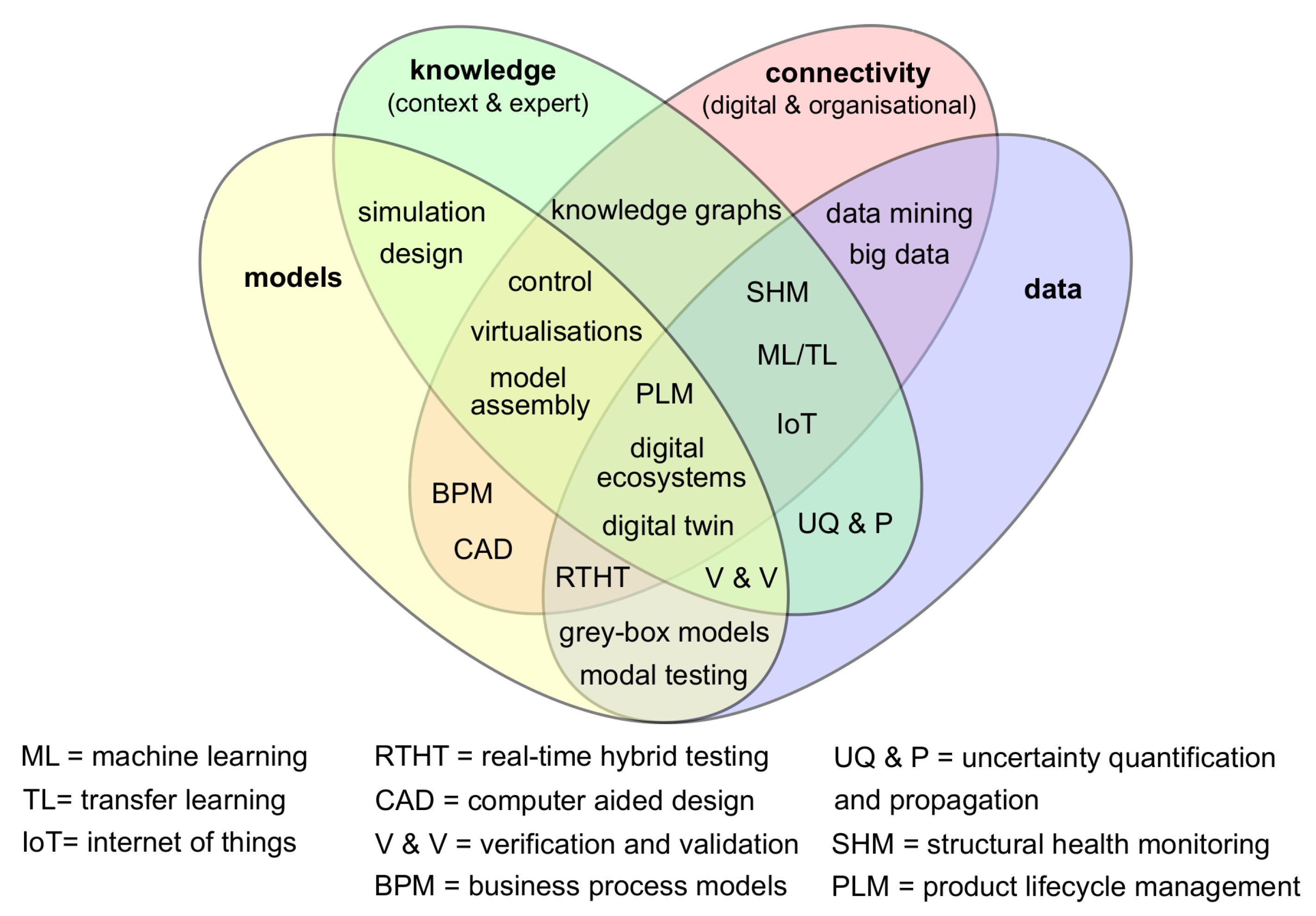
- Models: computational models based on physical reasoning;
- Data: both quantitive and qualitative sets of information from the physical twin;
- Knowledge: both in-depth expert understanding and context specific detail;
- Connectivity: time evolving digital and organisational interactions that are free from significant interruptions or other barriers.
2. Overview of the Digital Twin
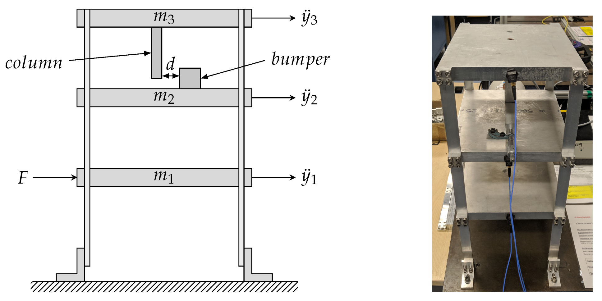
2.1. Experimental Data
2.2. Initial Validated Model
- 1.
- What does a digital twin do when predictive performance is poor?
- 2.
- How does a digital twin account for missing physics?
- 3.
- How does a digital twin learn new physics?
- 4.
- What is the impact on the control of the structure?
2.3. Proposed Digital Twin Model Structure
- Recalibrate the physics-based model: improve estimates of the model parameters.
- Update the data-based component: improve modelling of unknown physics.
- Addition of more physics: add new identified physics into the physics-based model.
- Do nothing.
3. The Problem of Model Updating
4. Data-Augmented Modelling
4.1. Gaussian Process Regression
4.2. Data-Based Model Component
4.3. Active Learning Approach
| Algorithm 1 Active learning for data-based component of a digital twin |
|
4.4. Autonomous Decision Making: Challenges and Limitations
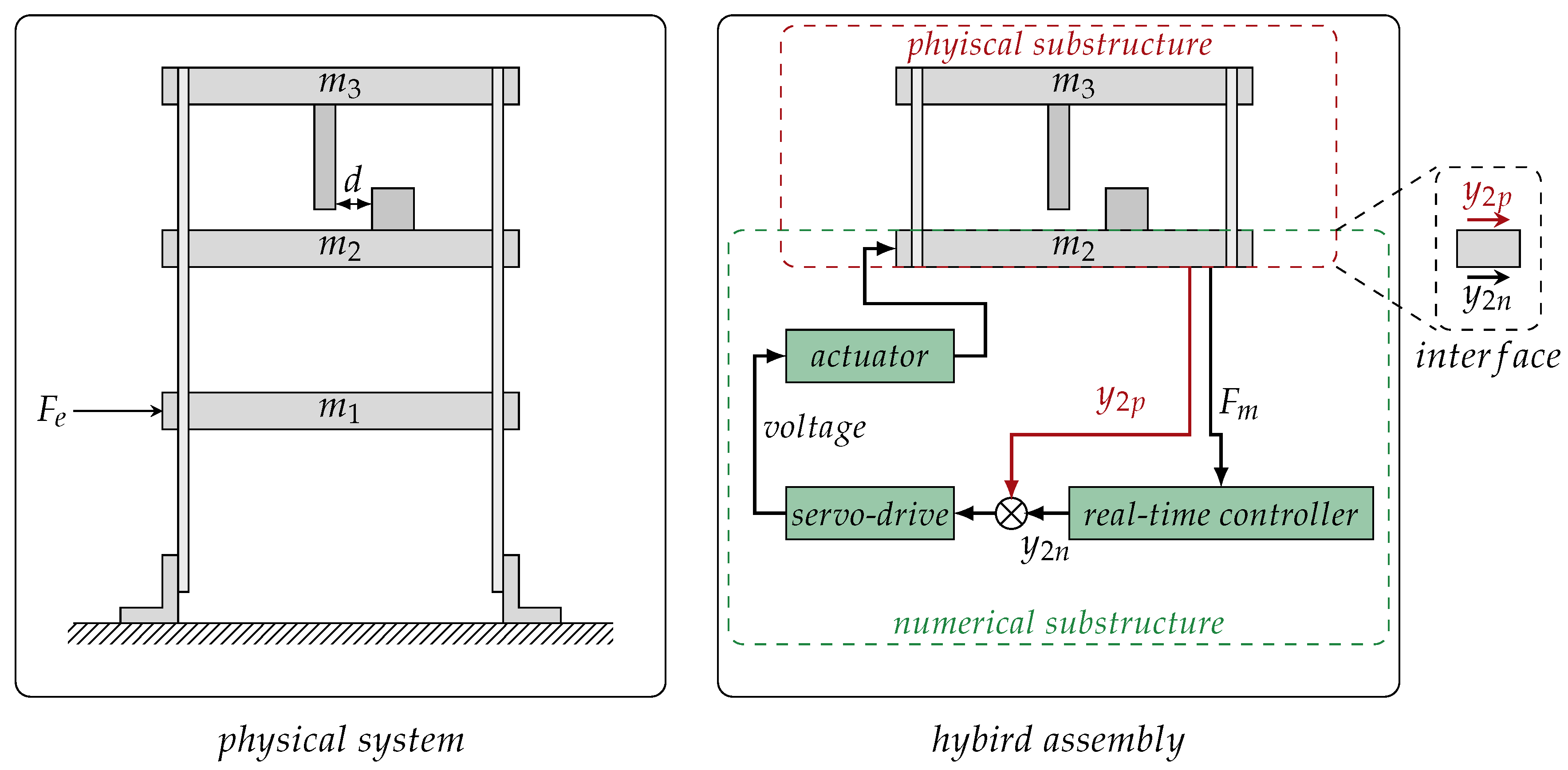
5. Identifying Physics through Hybrid Testing
6. Impact of a Digital Twin on Active Control
7. Discussion
8. Conclusions
Author Contributions
Funding
Conflicts of Interest
References
- Wagg, D.; Worden, K.; Barthorpe, R.; Gardner, P. Digital Twins: State-of-the-Art and Future Directions for Modeling and Simulation in Engineering Dynamics Applications. ASME J. Risk Uncertain. Part B 2020, 6, 030901. [Google Scholar] [CrossRef]
- Fuller, A.; Fan, Z.; Day, C.; Barlow, C. Digital Twin: Enabling Technologies, Challenges and Open Research. IEEE Access 2020. [Google Scholar] [CrossRef]
- Jones, D.; Snider, C.; Nassehi, A.; Yon, J.; Hicks, B. Characterising the Digital Twin: A systematic literature review. CIRP J. Manuf. Sci. Technol. 2020, 29, 36–52. [Google Scholar] [CrossRef]
- Lee, J.; Ni, J.; Djurdjanovic, D.; Qiu, H.; Liao, H. Intelligent prognostics tools and e-maintenance. Comput. Ind. 2006, 57, 476–489. [Google Scholar] [CrossRef]
- Cerrone, A.; Hochhalter, J.; Heber, G.; Ingraffea, A. On the effects of modeling as-manufactured geometry: Toward digital twin. Int. J. Aerosp. Eng. 2014, 2014, 439278. [Google Scholar] [CrossRef]
- Seshadri, B.R.; Krishnamurthy, T. Structural health management of damaged aircraft structures using digital twin concept. In Proceedings of the 25th AIAA/AHS Adaptive Structures Conference, Grapevine, TX, USA, 9–13 January 2017; p. 1675. [Google Scholar]
- Karve, P.M.; Guo, Y.; Kapusuzoglu, B.; Mahadevan, S.; Haile, M.A. Digital twin approach for damage-tolerant mission planning under uncertainty. Eng. Fract. Mech. 2020, 225, 106766. [Google Scholar] [CrossRef]
- Liu, Z.; Meyendorf, N.; Mrad, N. The role of data fusion in predictive maintenance using Digital Twin. AIP Conf. Proc. 2018, 1949, 020023. [Google Scholar]
- Aivaliotis, P.; Georgoulias, K.; Arkouli, Z.; Makris, S. Methodology for enabling digital twin using advanced physics-based modelling in predictive maintenance. Procedia CIRP 2019, 81, 417–422. [Google Scholar] [CrossRef]
- Werner, A.; Zimmermann, N.; Lentes, J. Approach for a Holistic Predictive Maintenance Strategy by Incorporating a Digital Twin. Procedia Manuf. 2019, 39, 1743–1751. [Google Scholar] [CrossRef]
- Kapteyn, M.G.; Knezevic, D.J.; Willcox, K. Toward predictive digital twins via component-based reduced-order models and interpretable machine learning. In Proceedings of the AIAA Scitech 2020 Forum, Orlando, FL, USA, 6–10 January 2020; p. 0418. [Google Scholar]
- Li, C.; Mahadevan, S.; Ling, Y.; Choze, S.; Wang, L. Dynamic Bayesian Network for Aircraft Wing Health Monitoring Digital Twin. AIAA J. 2017, 55, 930–941. [Google Scholar] [CrossRef]
- Grieves, M.; Vickers, J. Digital twin: Mitigating Unpredictable, Undesirable Emergent Behavior in Complex Systems. In Transdisciplinary Perspectives on Complex Systems; Springer: Cham, Switzerland, 2017; pp. 85–113. [Google Scholar]
- Worden, K.; Cross, E.; Barthorpe, R.; Wagg, D.; Gardner, P. On Digital Twins, Mirrors, and Virtualizations: Frameworks for Model Verification and Validation. ASME J. Risk Uncertain. Part B 2020, 6, 030902. [Google Scholar] [CrossRef]
- Sharma, P.; Hamedifar, H.; Brown, A.; Green, R. The Dawn of the New Age of the Industrial Internet and How it can Radically Transform the Offshore Oil and Gas Industry. In Proceedings of the Offshore Technology Conference, Houston, TX, USA, 1–4 May 2017. [Google Scholar]
- Wanasinghe, T.R.; Wroblewski, L.; Petersen, B.; Gosine, R.G.; James, L.A.; De Silva, O.; Mann, G.K.; Warrian, P.J. Digital Twin for the Oil and Gas Industry: Overview, Research Trends, Opportunities, and Challenges. IEEE Access 2020. [Google Scholar] [CrossRef]
- Sivalingam, K.; Sepulveda, M.; Spring, M.; Davies, P. A Review and Methodology Development for Remaining Useful Life Prediction of Offshore Fixed and Floating Wind turbine Power Converter with Digital Twin Technology Perspective. In Proceedings of the 2018 2nd International Conference on Green Energy and Applications (ICGEA), Singapore, 24–26 March 2018; IEEE: New York, NY, USA, 2018; pp. 197–204. [Google Scholar]
- Tygesen, U.T.; Jepsen, M.S.; Vestermark, J.; Dollerup, N.; Pedersen, A. The True Digital Twin Concept for Fatigue Re-Assessment of Marine Structures. In Proceedings of the ASME 2018 37th International Conference on Ocean, Offshore and Arctic Engineering, Madrid, Spain, 17–22 June 2018; American Society of Mechanical Engineers: New York, NY, USA, 2018; p. V001T01A021. [Google Scholar]
- Pargmann, H.; Euhausen, D.; Faber, R. Intelligent big data processing for wind farm monitoring and analysis based on cloud-technologies and digital twins: A quantitative approach. In Proceedings of the 2018 IEEE 3rd International Conference on Cloud Computing and Big Data Analysis (ICCCBDA), Chengdu, China, 20–22 April 2018; IEEE: New York, NY, USA, 2018; pp. 233–237. [Google Scholar]
- Oñederra, O.; Asensio, F.; Eguia, P.; Perea, E.; Pujana, A.; Martinez, L. MV Cable Modeling for Application in the Digital Twin of a Windfarm. In Proceedings of the 2019 International Conference on Clean Electrical Power (ICCEP), Otranto, Italy, 2–4 July 2019; IEEE: New York, NY, USA, 2019; pp. 617–622. [Google Scholar]
- Glaessgen, E.H.; Stargel, D. The Digital Twin paradigm for future NASA and US Air Force vehicles. In Proceedings of the 53rd Structures, Structural Dynamics and Materials Conference, Honolulu, HI, USA, 23–26 April 2012; pp. 1–14. [Google Scholar]
- Zaccaria, V.; Stenfelt, M.; Aslanidou, I.; Kyprianidis, K.G. Fleet monitoring and diagnostics framework based on digital twin of aero-engines. In Proceedings of the Turbo Expo: Power for Land, Sea, and Air, Oslo, Norway, 11–15 June 2018; American Society of Mechanical Engineers: New York, NY, USA, 2018; Volume 51128, p. V006T05A021. [Google Scholar]
- Dawes, W.N.; Meah, N.; Kudryavtsev, A.; Evans, R.; Hunt, M.; Tiller, P. Digital Geometry to Support a Gas Turbine Digital Twin. In Proceedings of the AIAA Scitech 2019 Forum, San Diego, CA, USA, 7–11 January 2019; p. 1715. [Google Scholar]
- Patterson, E.A.; Taylor, R.J.; Bankhead, M. A framework for an integrated nuclear digital environment. Prog. Nucl. Energy 2016, 87, 97–103. [Google Scholar] [CrossRef]
- Iglesias, D.; Bunting, P.; Esquembri, S.; Hollocombe, J.; Silburn, S.; Vitton-Mea, L.; Balboa, I.; Huber, A.; Matthews, G.; Riccardo, V.; et al. Digital twin applications for the JET divertor. Fusion Eng. Des. 2017, 125, 71–76. [Google Scholar] [CrossRef]
- Volodin, V.; Tolokonskii, A. Concept of instrumentation of digital twins of nuclear power plants units as observers for digital NPP I&C system. J. Phys. Conf. Ser. 2019, 1391, 012083. [Google Scholar]
- Chatzis, M.; Chatzi, E.; Triantafyllou, S. A Discontinuous Extended Kalman Filter for non-smooth dynamic problems. Mech. Syst. Signal Process. 2017, 92, 13–29. [Google Scholar] [CrossRef] [Green Version]
- Kim, J.; Lynch, J.P. Subspace system identification of support excited structures—part II: Gray-box interpretations and damage detection. Earthq. Eng. Struct. Dyn. 2012, 41, 2253–2271. [Google Scholar] [CrossRef] [Green Version]
- Chatzis, M.; Chatzi, E.; Smyth, A. An experimental validation of time domain system identification methods with fusion of heterogeneous data. Earthq. Eng. Struct. Dyn. 2015, 44, 523–547. [Google Scholar] [CrossRef]
- Beck, J.L.; Katafygiotis, L.S. Updating models and their uncertainties. I: Bayesian statistical framework. J. Eng. Mech. 1998, 124, 455–461. [Google Scholar] [CrossRef]
- Katafygiotis, L.S.; Beck, J.L. Updating models and their uncertainties. II: Model identifiability. J. Eng. Mech. 1998, 124, 463–467. [Google Scholar] [CrossRef]
- Mottershead, J.E.; Link, M.; Friswell, M.I. The sensitivity method in finite element model updating: A tutorial. Mech. Syst. Signal Process. 2011, 25, 2275–2296. [Google Scholar] [CrossRef]
- Simoen, E.; De Roeck, G.; Lombaert, G. Dealing with uncertainty in model updating for damage assessment: A review. Mech. Syst. Signal Process. 2015, 56, 123–149. [Google Scholar] [CrossRef] [Green Version]
- Chatzi, E.N.; Smyth, A.W. Particle filter scheme with mutation for the estimation of time-invariant parameters in structural health monitoring applications. Struct. Control Health Monit. 2013, 20, 1081–1095. [Google Scholar] [CrossRef]
- Kennedy, M.C.; O’Hagan, A. Bayesian calibration of computer models. J. R. Stat. Soc. Ser. B (Stat. Methodol. 2001, 63, 425–464. [Google Scholar] [CrossRef]
- Berger, J.O.; Cavendish, J.; Paulo, R.; Lin, C.H.; Cafeo, J.A.; Sacks, J.; Bayarri, M.J.; Tu, J. A framework for validation of computer models. Technometrics 2007, 49, 138–154. [Google Scholar]
- Brynjarsdóttir, J.; O’Hagan, A. Learning about physical parameters: The importance of model discrepancy. Inverse Probl. 2014, 30, 114007. [Google Scholar] [CrossRef]
- Vapnik, V.N. The Nature of Statistical Learning Theory; Springer: New York, NY, USA, 1999. [Google Scholar]
- Bishop, C.M. Neural Networks for Pattern Recognition; Oxford University Press, Inc.: New York, NY, USA, 1995. [Google Scholar]
- LeCun, Y.; Bengio, Y.; Hinton, G. Deep learning. Nature 2015, 521, 436–444. [Google Scholar] [CrossRef]
- Rasmussen, C.E.; Williams, C.K.I. Gaussian Processes for Machine Learning; MIT Press: Cambridge, MA, USA, 2006. [Google Scholar]
- Stein, M.L. Interpolation of Spatial Data: Some Theory for Kriging; Springer Series in Statistics; Springer: New York, NY, USA, 1999. [Google Scholar]
- Worden, K.; Surace, C.; Becker, W. Uncertainty bounds on higher-order FRFs from Gaussian process NARX models. Procedia Eng. 2017, 199, 1994–2000. [Google Scholar] [CrossRef]
- Worden, K.; Becker, W.; Rogers, T.; Cross, E. On the confidence bounds of Gaussian process NARX models and their higher-order frequency response functions. Mech. Syst. Signal Process. 2018, 104, 188–223. [Google Scholar] [CrossRef]
- Enqvist, M.; Ljung, L. Linear approximations of nonlinear FIR systems for separable input processes. Automatica 2005, 41, 459–473. [Google Scholar] [CrossRef] [Green Version]
- Settles, B. Active Learning Lliterature Survey. In Computer Sciences Technical Report; University of Wisconsin–Madison: Madison, WI, USA, 2009. [Google Scholar]
- Bull, L.; Worden, K.; Manson, G.; Dervilis, N. Active learning for semi-supervised structural health monitoring. J. Sound Vib. 2018, 437, 373–388. [Google Scholar] [CrossRef]
- Ho, S.; Wechsler, H. Query by transduction. IEEE Trans. Pattern Anal. Mach. Intell. 2008, 30, 1557–1571. [Google Scholar] [PubMed]
- Loy, C.C.; Hospedales, T.M.; Xiang, T.; Gong, S. Stream-based joint exploration-exploitation active learning. In Proceedings of the 2012 IEEE Conference on Computer Vision and Pattern Recognition, Providence, RI, USA, 16–21 June 2012; pp. 1560–1567. [Google Scholar]
- Bedford, T.; Cooke, R. Probabilistic Risk Analysis: Foundations and Methods; Cambridge University Press: Cambridge, UK, 2001. [Google Scholar]
- Berger, J. Statistical Decision Theory and Bayesian Analysis; Springer: New York, NY, USA, 1985. [Google Scholar]
- Snelson, E.; Ghahramani, Z. Sparse Gaussian processes using pseudo-inputs. In Proceedings of the Advances in Neural Information Processing Systems, Vancouver, BC, Canada, 5–8 December 2005. [Google Scholar]
- Titsias, M. Variational learning of inducing variables in sparse Gaussian processes. In Proceedings of the International Conference on Artificial Intelligence and Statistics, Clearwater, FL, USA, 16–19 April 2009. [Google Scholar]
- Bui, T.D.; Yan, J.; Turner, R.E. A unifying framework for Gaussian process pseudo-point approximations using power expectation propagation. J. Mach. Learn. Res. 2017, 18, 3649–3720. [Google Scholar]
- Bijl, H.; van Wingerden, J.W.; Schön, T.B.; Verhaegen, M. Online sparse Gaussian process regression using FITC and PITC approximations. IFAC 2015, 48, 703–708. [Google Scholar]
- Bui, T.D.; Nguyen, C.; Turner, R.E. Streaming Sparse Gaussian Process Approximations. In Proceedings of the Advances in Neural Information Processing Systems, Long Beach, CA, USA, 4–9 December 2017; pp. 3299–3307. [Google Scholar]
- Wagg, D.; Neild, S.; Gawthrop, P. Real-Time Testing with Dynamic Substructuring. In Modern Testing Techniques for Structural Systems; Springer: Wien, Austria, 2008; Volume 502. [Google Scholar]
- Horiuchi, T.; Inoue, M.; Konno, T.; Namita, Y. Real-time hybrid experimental system with actuator delay compensation and its application to a piping system with energy absorber. Earthq. Eng. Struct. Dyn. 1999, 28, 1121–1141. [Google Scholar] [CrossRef]
- Preumont, A. Vibration Control of Active Structures; Springer: Berlin, Germany, 1997; Volume 2. [Google Scholar]
- Fuentes, R.; Dervilis, N.; Worden, K.; Cross, E. Efficient parameter identification and model selection in nonlinear dynamical systems via sparse Bayesian learning. J. Phys. Conf. Ser. 2019, 1264, 012050. [Google Scholar] [CrossRef]
- Beck, J.L.; Yuen, K.V. Model Selection Using Response Measurements: Bayesian Probabilistic Approach. J. Eng. Mech. 2004, 130, 192–203. [Google Scholar] [CrossRef]


 ), model prediction (
 ), (green shaded region), residual error (
 ).
), model prediction (), (green shaded region), residual error ().
).
), model prediction (), (green shaded region), residual error ().
 ), model prediction (
 ), (green shaded region), residual error (
 ).
), model prediction (), (green shaded region), residual error ().
).
), model prediction (), (green shaded region), residual error ().
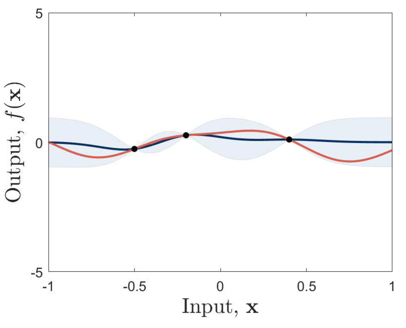
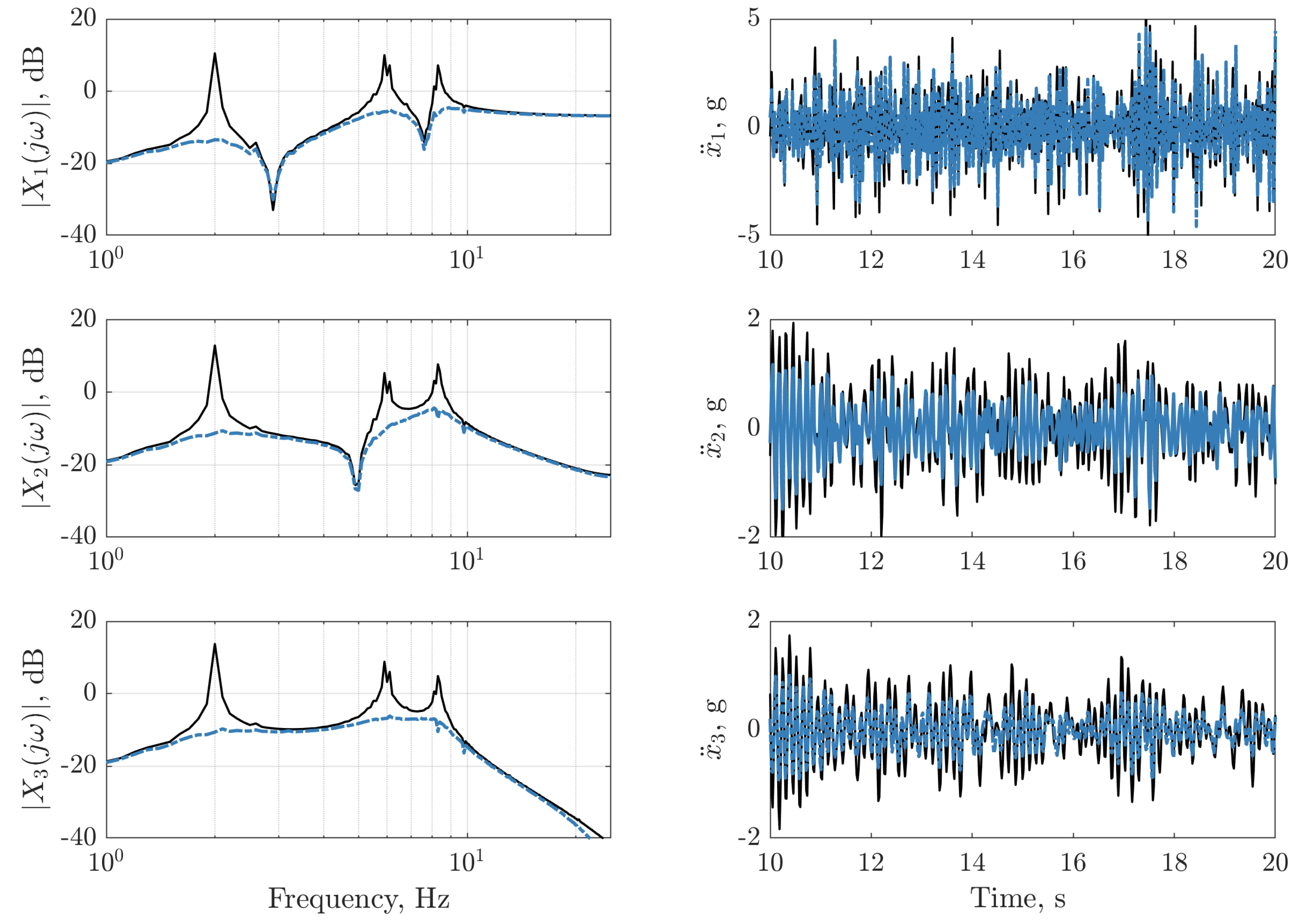
 ), predictive mean (
 ) and standard deviation, (blue shaded region), are shown.
), predictive mean () and standard deviation, (blue shaded region), are shown.
) and standard deviation, (blue shaded region), are shown.
), predictive mean () and standard deviation, (blue shaded region), are shown.
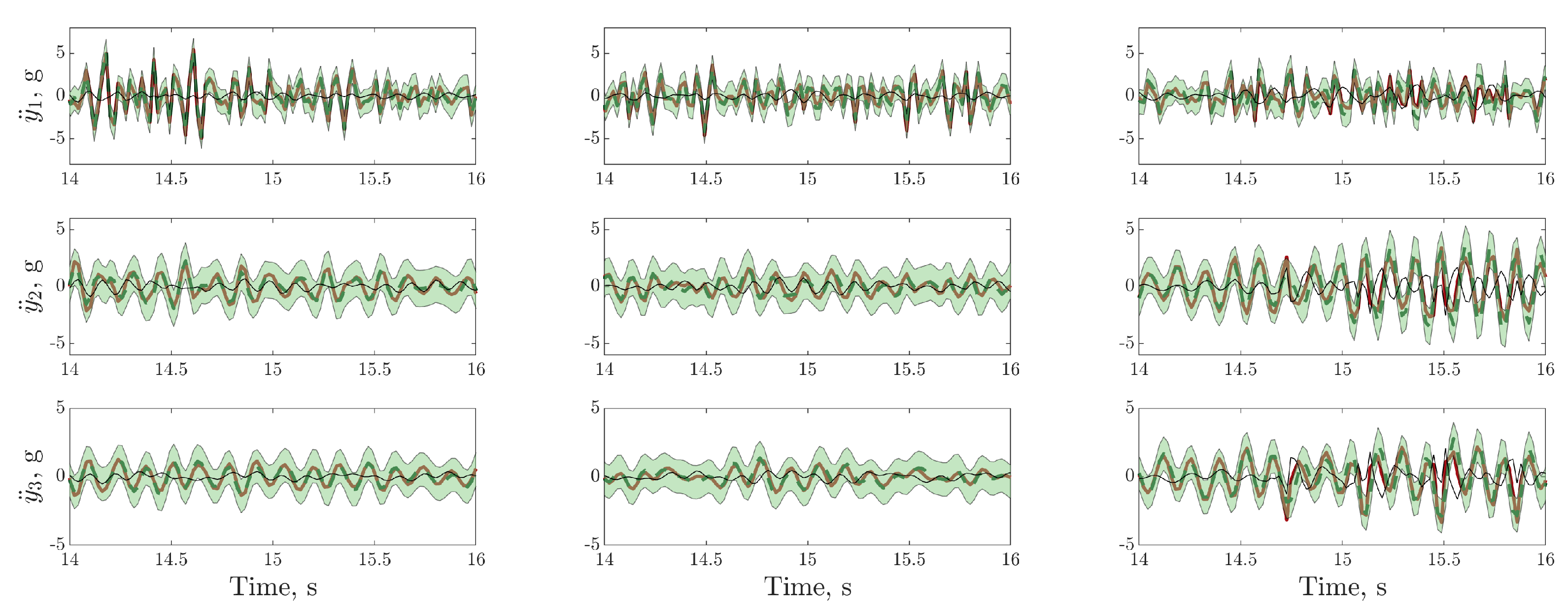
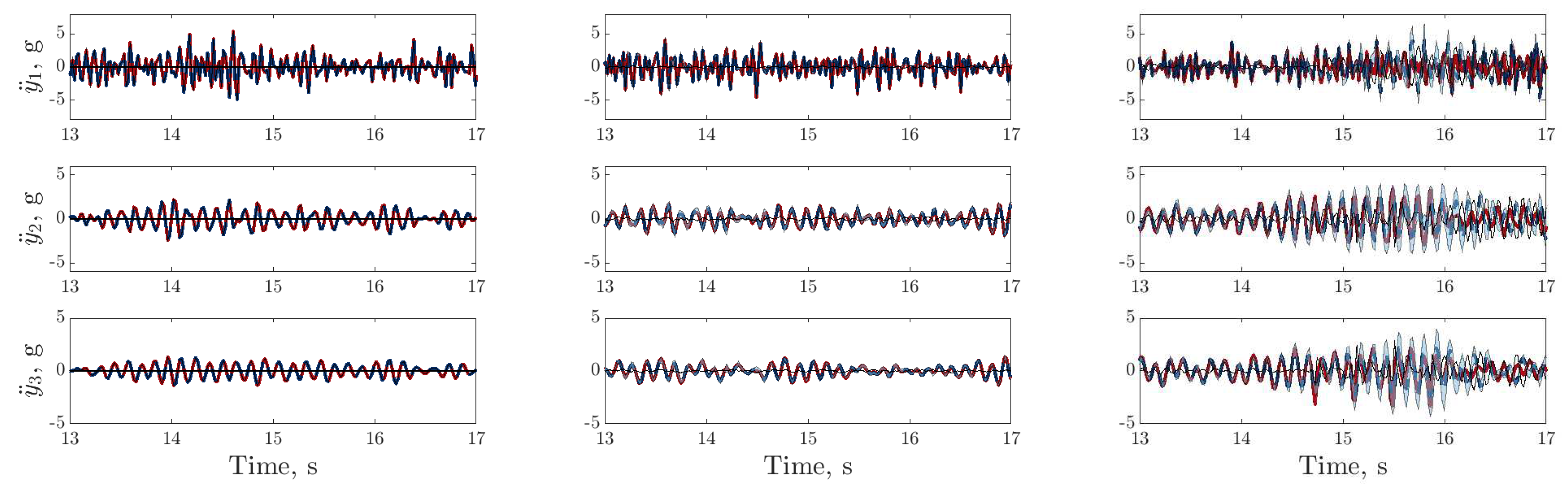
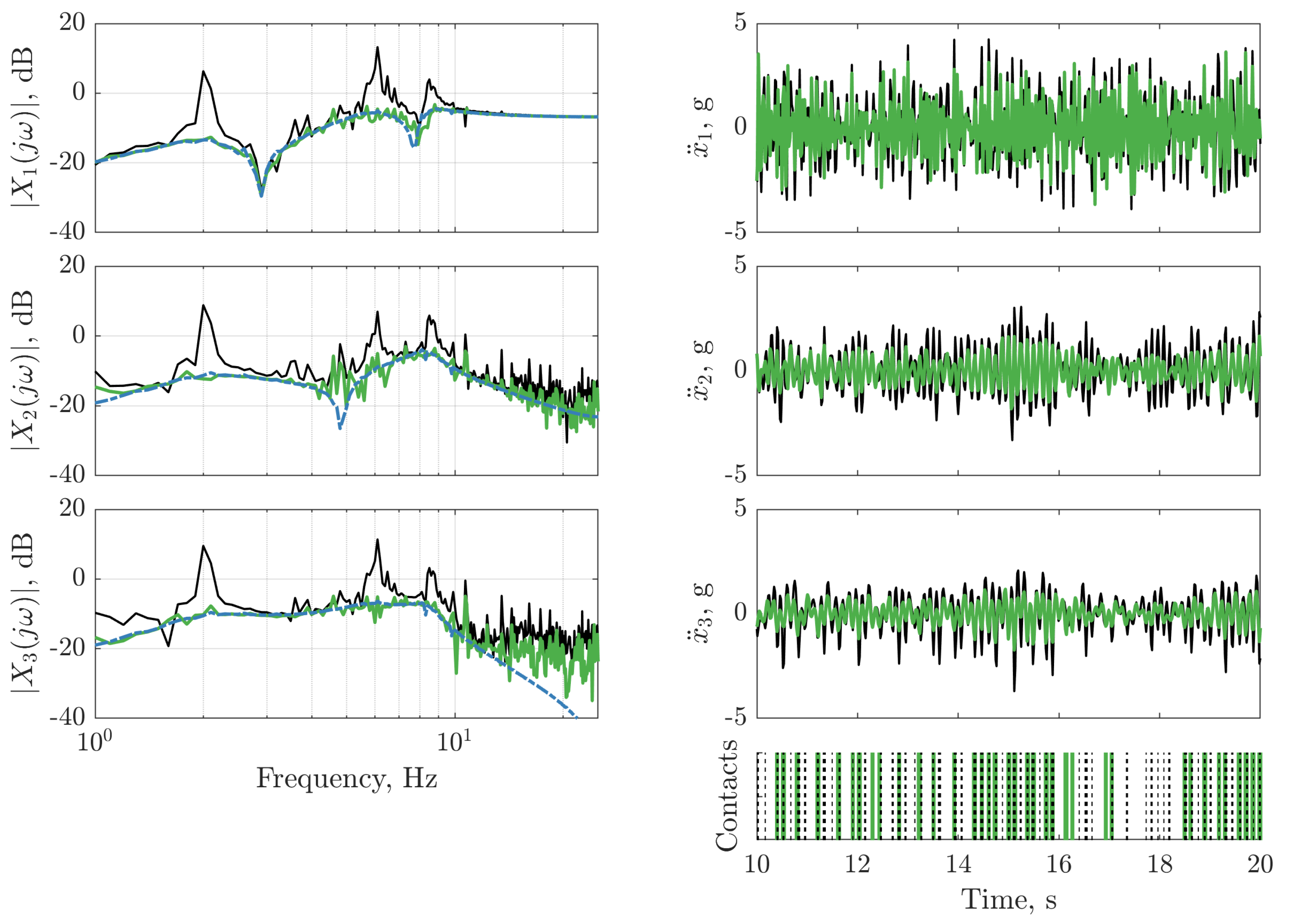
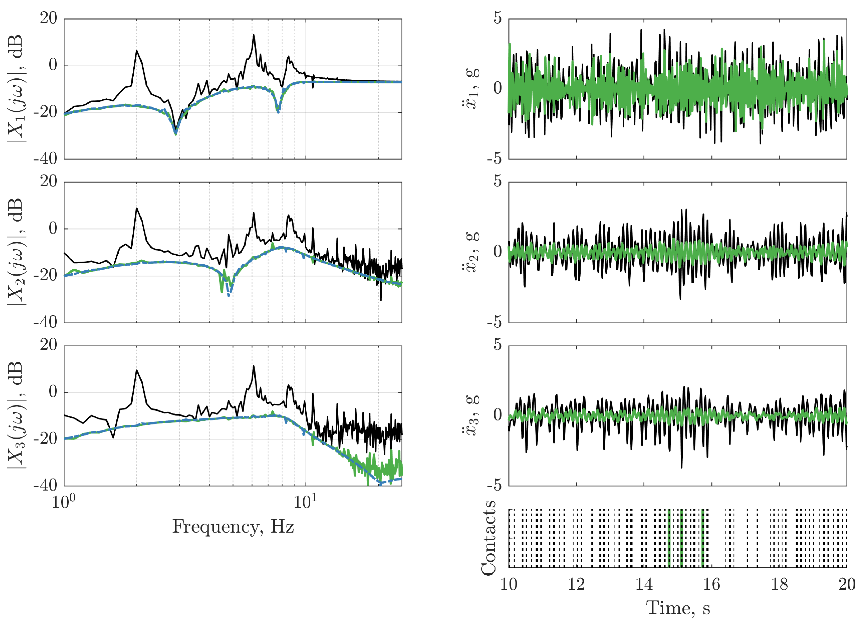
 ), digital twin mean prediction (
  ), digital twin confidence intervals (blue shaded region), residual error (
 ).
), digital twin mean prediction ( ), digital twin confidence intervals (blue shaded region), residual error ().
).
), digital twin mean prediction ( ), digital twin confidence intervals (blue shaded region), residual error ().
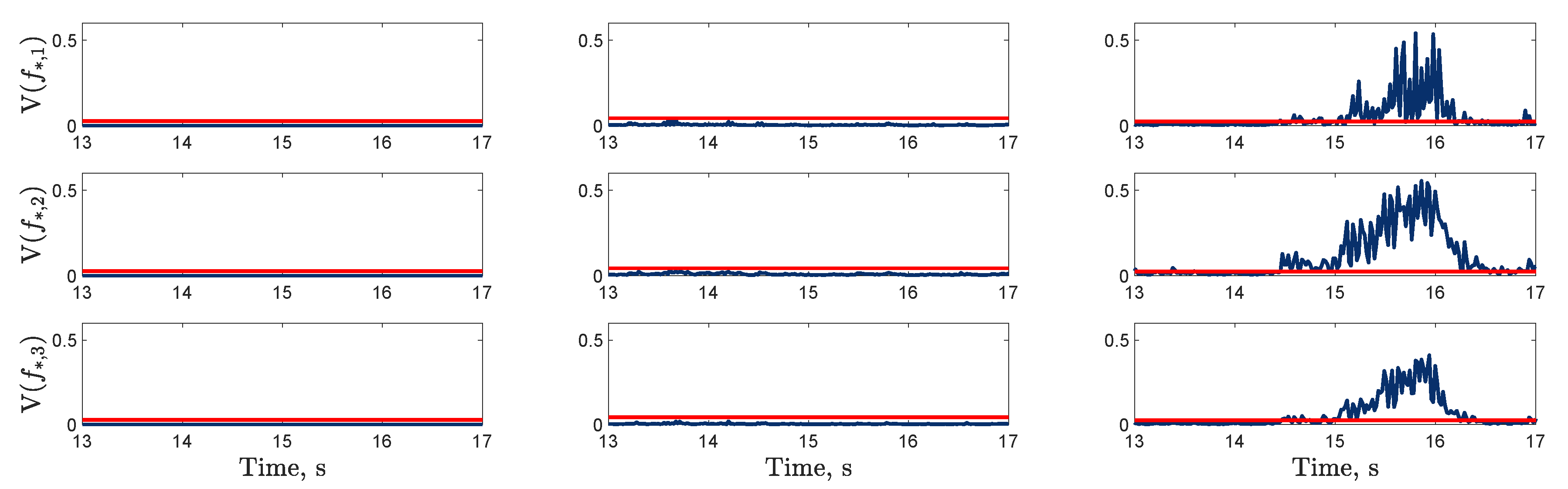
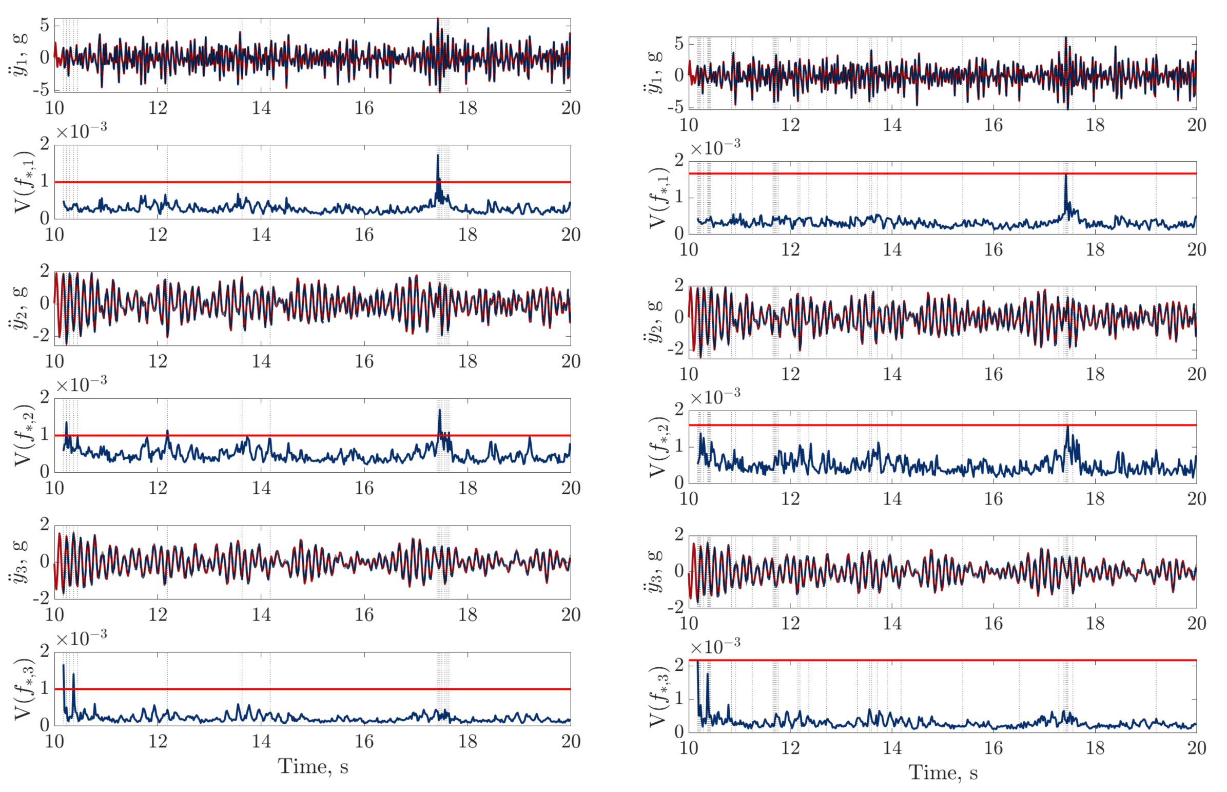
 ), trained using dataset one , between 13 and 17s on datasets one to three (left to right); threshold (
 ) determined by the maximum variance from the first 100 data points on dataset two.
), trained using dataset one , between 13 and 17s on datasets one to three (left to right); threshold () determined by the maximum variance from the first 100 data points on dataset two.
) determined by the maximum variance from the first 100 data points on dataset two.
), trained using dataset one , between 13 and 17s on datasets one to three (left to right); threshold () determined by the maximum variance from the first 100 data points on dataset two.


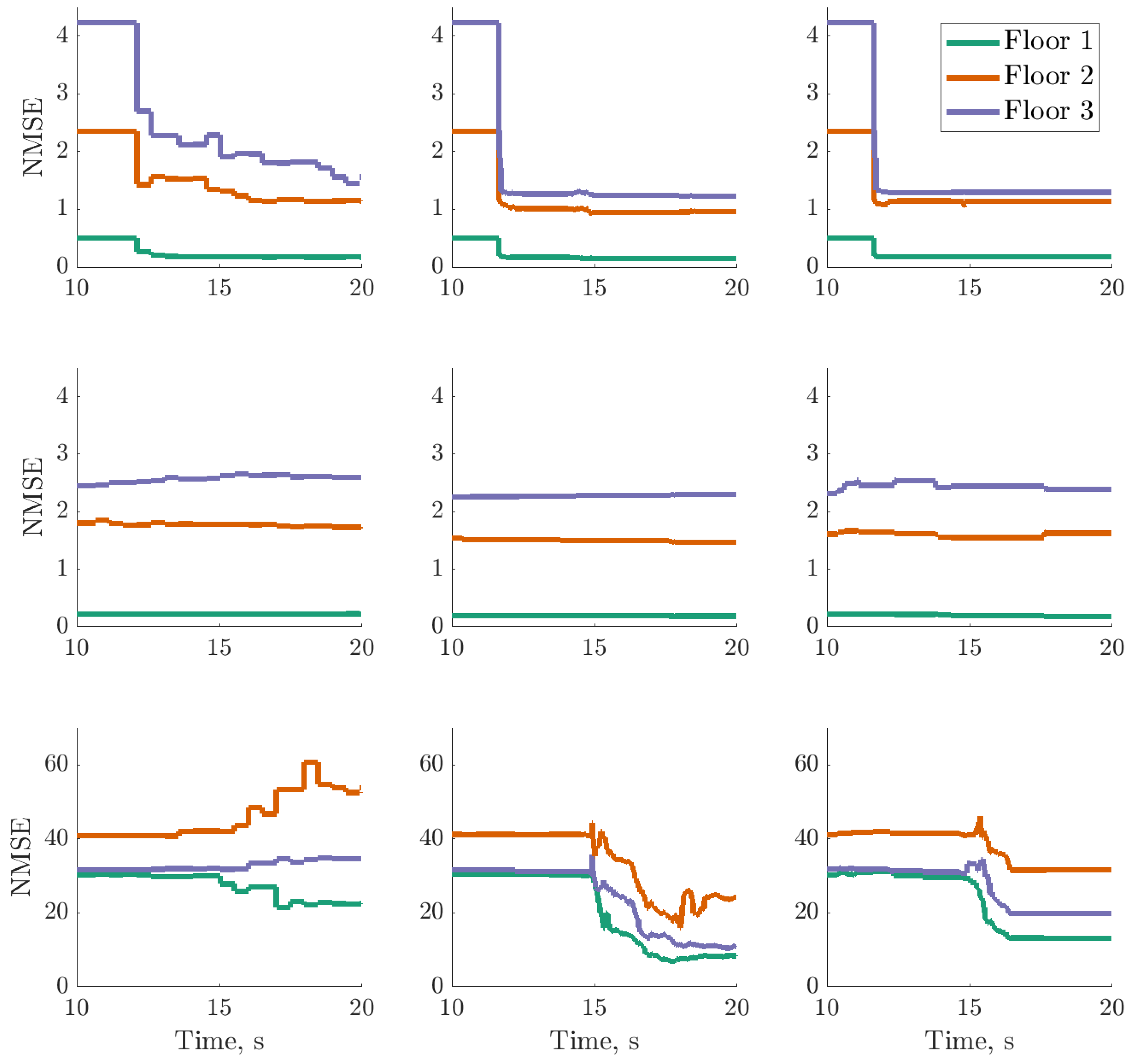
 ), digital twin mean prediction (
 ) and digital twin confidence intervals (blue shaded region) (top sub-panels), with the predictive variance (
 ) and final threshold (
 ) in the bottom sub-panels.
), digital twin mean prediction () and digital twin confidence intervals (blue shaded region) (top sub-panels), with the predictive variance () and final threshold () in the bottom sub-panels.
) in the bottom sub-panels.
), digital twin mean prediction () and digital twin confidence intervals (blue shaded region) (top sub-panels), with the predictive variance () and final threshold () in the bottom sub-panels.
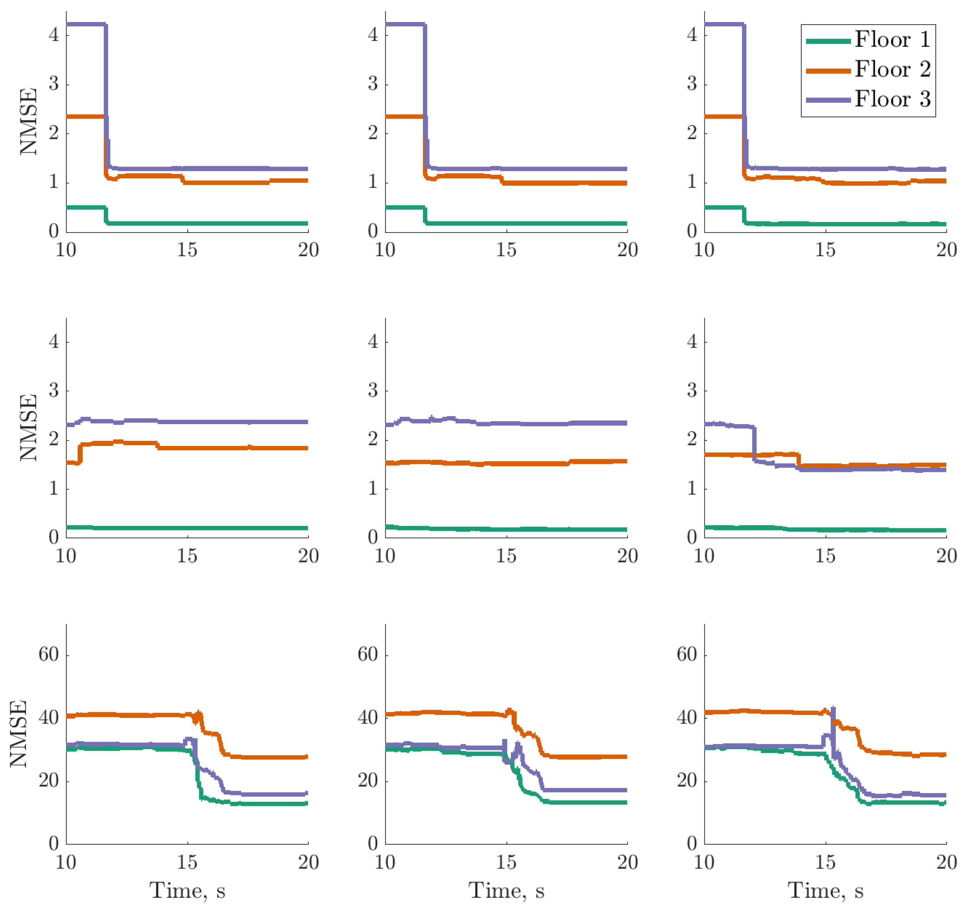
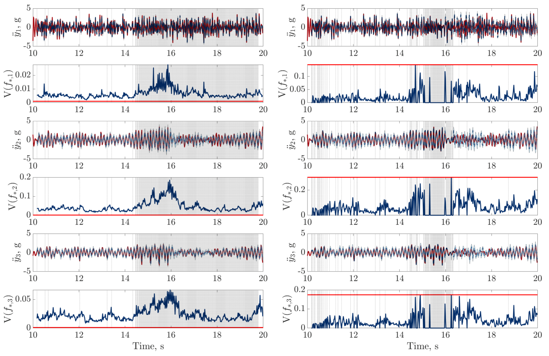


 ), and with LQR controller (
 ).
), and with LQR controller ().
).
), and with LQR controller ().
 ), and with LQR controller (
 ). The frequency response function of the LQR controller on dataset two (
 ) is depicted (left panels) for reference. The vertical lines on the bottom right panel indicate instances where the nonlinearity is triggered for the passive structure (:) and the structure with the LQR controller (
 ).
), and with LQR controller (). The frequency response function of the LQR controller on dataset two () is depicted (left panels) for reference. The vertical lines on the bottom right panel indicate instances where the nonlinearity is triggered for the passive structure (:) and the structure with the LQR controller ().
).
), and with LQR controller (). The frequency response function of the LQR controller on dataset two () is depicted (left panels) for reference. The vertical lines on the bottom right panel indicate instances where the nonlinearity is triggered for the passive structure (:) and the structure with the LQR controller ().
 ), and with the updated LQR controller (
 ). The frequency response function of the LQR controller on dataset two (
 ) is depicted (left panels) for reference. The vertical lines on the bottom right panels indicate instances where the nonlinearity is triggered for the passive structure (:) and the structure with the updated LQR controller (
 ).
), and with the updated LQR controller (). The frequency response function of the LQR controller on dataset two () is depicted (left panels) for reference. The vertical lines on the bottom right panels indicate instances where the nonlinearity is triggered for the passive structure (:) and the structure with the updated LQR controller ().
).
), and with the updated LQR controller (). The frequency response function of the LQR controller on dataset two () is depicted (left panels) for reference. The vertical lines on the bottom right panels indicate instances where the nonlinearity is triggered for the passive structure (:) and the structure with the updated LQR controller ().

| Masses, m | Damping Coefficients, c | Stiffness Coefficients, k | Signal Noises, | |
|---|---|---|---|---|
| kg | Ns/m | N/m | (g/N) 2 | |
| Dataset | Uniform | Fixed | ||||
|---|---|---|---|---|---|---|
| One | 18 | 69 | 11 | 14 | 17 | 40 |
| Two | 21 | 16 | 21 | 18 | 37 | 71 |
| Three | 21 | 280 | 98 | 115 | 106 | 135 |
© 2020 by the authors. Licensee MDPI, Basel, Switzerland. This article is an open access article distributed under the terms and conditions of the Creative Commons Attribution (CC BY) license (http://creativecommons.org/licenses/by/4.0/).
Share and Cite
Gardner, P.; Dal Borgo, M.; Ruffini, V.; Hughes, A.J.; Zhu, Y.; Wagg, D.J. Towards the Development of an Operational Digital Twin. Vibration 2020, 3, 235-265. https://doi.org/10.3390/vibration3030018
Gardner P, Dal Borgo M, Ruffini V, Hughes AJ, Zhu Y, Wagg DJ. Towards the Development of an Operational Digital Twin. Vibration. 2020; 3(3):235-265. https://doi.org/10.3390/vibration3030018
Chicago/Turabian StyleGardner, Paul, Mattia Dal Borgo, Valentina Ruffini, Aidan J. Hughes, Yichen Zhu, and David J. Wagg. 2020. "Towards the Development of an Operational Digital Twin" Vibration 3, no. 3: 235-265. https://doi.org/10.3390/vibration3030018