Zonal Turbulence Modeling Approach for Simulating Compartment Fire for Initial Hazard Assessment

Abstract

The flow field driven by a compartment fire usually contains several flow zones with different physical structures. As each type of turbulence model has its own predominant application area, it is logical to apply two or more simple turbulence models to the same fire-induced flow field at different locations according to their predominant features to yield a comparatively simple, accurate, and stable zonal turbulence model. A zonal turbulence model, which is a hybrid of the standard k-ε model and its modification, is developed in this paper. The model is tested and compared with the experimental data. A promising improvement is observed when comparing it with the base turbulence model, i.e., the standard k-ε model, especially in the recirculating region near the corners of the compartment. This approach in having different zones in the plume region will be useful for handling more scenarios at the initial stage of fire hazard assessments.

1. Introduction

In studying compartmental fires, the fire-induced flow is almost always turbulent. That means the fluid motion is highly random, unsteady, and three-dimensional. Due to these complexities, turbulent motion and heat, and the mass transfer associated with it, are extremely difficult to describe and predict theoretically.

At present, in spite of all the recent advances in computer technology, turbulent flows cannot be calculated with an exact method. Therefore, a numerical approach is required to solve this type of problem.

Computational fluid dynamics or field modeling is one of the numerical methods for predicting the fire-induced flow [1,2]. Field modeling is based on the conservation laws for mass, momentum, and energy. The basic conservation laws are expressed by the exact equations describing all the details of the fluid motion. The details of the fluctuating motion are not the topic of interest. A statistical approach was taken and the equations were averaged over a time scale which is long compared with that of the turbulent motion. The resulting equations describing the distribution of the mean velocity, pressure, temperature, and species concentration in the flow and, thus, the quantities are of prime interest. Unfortunately, the process of averaging has created a new problem. The set of equations does not constitute a closed system since the equations contain unknown terms, $\overline{u^{\prime }{}_i{\varphi }^{\prime }{}_{}}$, representing the transport of mean momentum, heat, and mass by the turbulent motion. The system can only be solved with the aid of a suitable turbulence model.

Turbulent transport processes are strongly dependent on the geometrical conditions, fluid property, and flow pattern. Turbulence models can only give an approximate description with a particular set of empirical constants which are valid only for a certain flow, or in some range of flows. In practical applications, the more universal turbulence models are usually more complex and unstable, thus requiring more computing time.

Computational fluid dynamics (CFD) with large-eddy simulation (LES) has been used [3,4,5,6,7,8,9,10,11,12,13,14] in fire hazard assessments for many years. Most of the CFD fire models are not properly validated with systematic large-scale fire tests with criticisms. Simulations with LES will take a very long central processing unit (CPU) time even when linking with a fast computer with expensive costs. This is not appropriate for a hazard assessment, with thousands of scenarios to simulate. A zone model was then used for preliminary studies before large-scale simulations and full-scale burning tests. Fire hazard assessments in nuclear facilities involving a burning cable [15] is a good example. A modified Reynolds-averaged Navier–Stokes (RANS) model with faster simulation times is then proposed, which might be better than using the zone model through symbolic mathematics [16].

In a compartmental fire, the flow field can be divided into several regions by its own distinct feature and property. Each region can be simulated successfully with a suitable type of turbulence model. Theoretically, if several turbulence models are employed locally to simulate the fire-induced flow field, according to the predominant feature of each model, the predicted results should be good and computationally cheap.

In this paper, this zone-modeling approach is applied to study compartment fires using CFD. It will be compared with the standard k-ε model for the application in fire-field modeling. Their performance will be assessed in terms of the accuracy of the predicted results of the air flow pattern and temperature distribution induced by a fire in a compartment.

2. Zonal Turbulence Model

A complex flow field usually contains several flow zones with different physical structures. Since the attempts to construct a universal turbulence model may cause convergence problems and require much computational resources [17,18], it seems logical to construct a zonal turbulence model in which each flow zone is modeled independently. In the zonal modeling strategy, each different zone is identified separately, since it should be easier to construct accurate models for a zone than for the flow field as a whole. As a result, a zonal model can be much simpler than a universal turbulence model for achieving a given level of accuracy.

2.1. Continuity Problem

When a flow field is decomposed into different zones, there exist regions between the zones where one zone changes into another. Physically, the transition from one type of structure to another may cause a discontinuity problem. In order to minimize the difficulty of blending, the models for various zones should have the same form. From Chow and Mok [19], a serious blending problem is identified between fundamentally different turbulence models, such as the combination of a two-equation-type turbulence model and a zero-equation-type turbulence model. However, the discontinuity problem becomes insignificant when the combination of a modified form of the k-ε turbulence models is applied.

2.2. Methodology

In order to construct a zonal turbulence model, a simple and stable turbulence model was first used for the whole flow field. Such a model is called a base model. The standard k-ε model was employed as the base turbulence model in this study since it is well-known to be fast-running, simple, and stable with reasonable accuracy [20,21,22,23]. According to the computed results, i.e., flow field and temperature field, different flow regions can be located without difficulty. In each region, the flow structure was analyzed to understand why the base turbulence model was inaccurate. Then, modification of the base turbulence model can be targeted to different flow regions with respect to their distinct features. By combining all different localized modifications, a suitable and comparatively simple zonal turbulence model is formed. The methodology of zonal turbulence modeling is summarized as follows:

(a)

Select a base turbulence model;

(b)

Compute the flow field with the base turbulence model;

(c)

From the predicted results, such as flow field and temperature field, different flow zones are identified;

(d)

Modify the base model for these zones accordingly with a specific and simple turbulence model;

(e)

Compute the flow field with the proposed zonal turbulence model.

2.3. Different Flow Regions

From the fire anatomy, the flow field of most of the compartmental fires can be divided into several regions [24], i.e., fire plume region, flow entrainment region, and recirculating region. When studying the fire-induced flow field in more detail, the flow regions are not limited to these three areas. However, these three regions are considered more representative and can be described successfully by the available turbulence models in the present paper.

The fire plume region is situated above the fire seat. A high velocity, temperature, and Reynolds number are expected. This region is highly dependent on the position of the seat of the fire source and the compartment geometry.

The flow entrainment region is situated beside the fire plume region. Due to the velocity and pressure of the fire plume region, a lot of air is entrained into the fire plume region. A great velocity difference and pressure difference are expected.

The recirculating region is highly related to the fire plume flow direction, fluid property, compartment geometry, and position of the air inlet/outlet. The recirculating region always appears in the cavity of the compartment just beside the entrainment region, at the sharp corner of the compartment and near the air inlet/outlet.

Each region has its own characteristics which can be predicted with better accuracy by a suitable turbulence model [25]. For example, the recirculating region should not be classified as a region with isotropic turbulence. Otherwise, the values of the turbulence viscosity would be overestimated [25,26,27]. Further, the reversed flow would make a positive contribution to the turbulence shear stress [27]. Different turbulence models are proposed to be used in different regions.

2.4. Fire Source

According to a review on the chemical reactions of burning Poly(methyl methacrylate) (PMMA) with the simple kinetics of thermal decomposition [28], there are three stages in the combustion process: PMMA decomposes to produce monomer methylmethacrylate (MMA); monomer MMA decomposes to generate small gaseous molecules; and these small molecules undergo combustion. Intermediate chemical reactions are very complex with seven group reactions: thermal decomposition; thermal oxidative decomposition; decomposition of monomer MMA; methane combustion; methanol combustion; formaldehyde combustion; and acetylene combustion. There are thousands of reactions to model, for example, 26 species and 77 elementary reactions in methane combustion. The reaction mechanism of acetylene has 103 elementary reactions and 38 species. As combustion chemistry is too complicated to be involved and this study is on turbulent flow, the fire source is taken as a heat source with a specified thermal power.

3. Fire-Field Modeling

The technique of computational fluid dynamics (field modeling) is applied to simulate fires in a compartment. The flow is turbulent in nature, and the values of the flow variables are solved. The induced flow and temperature field can be described by a set of equations derived from the law of conservation of mass, momentum, and enthalpy. 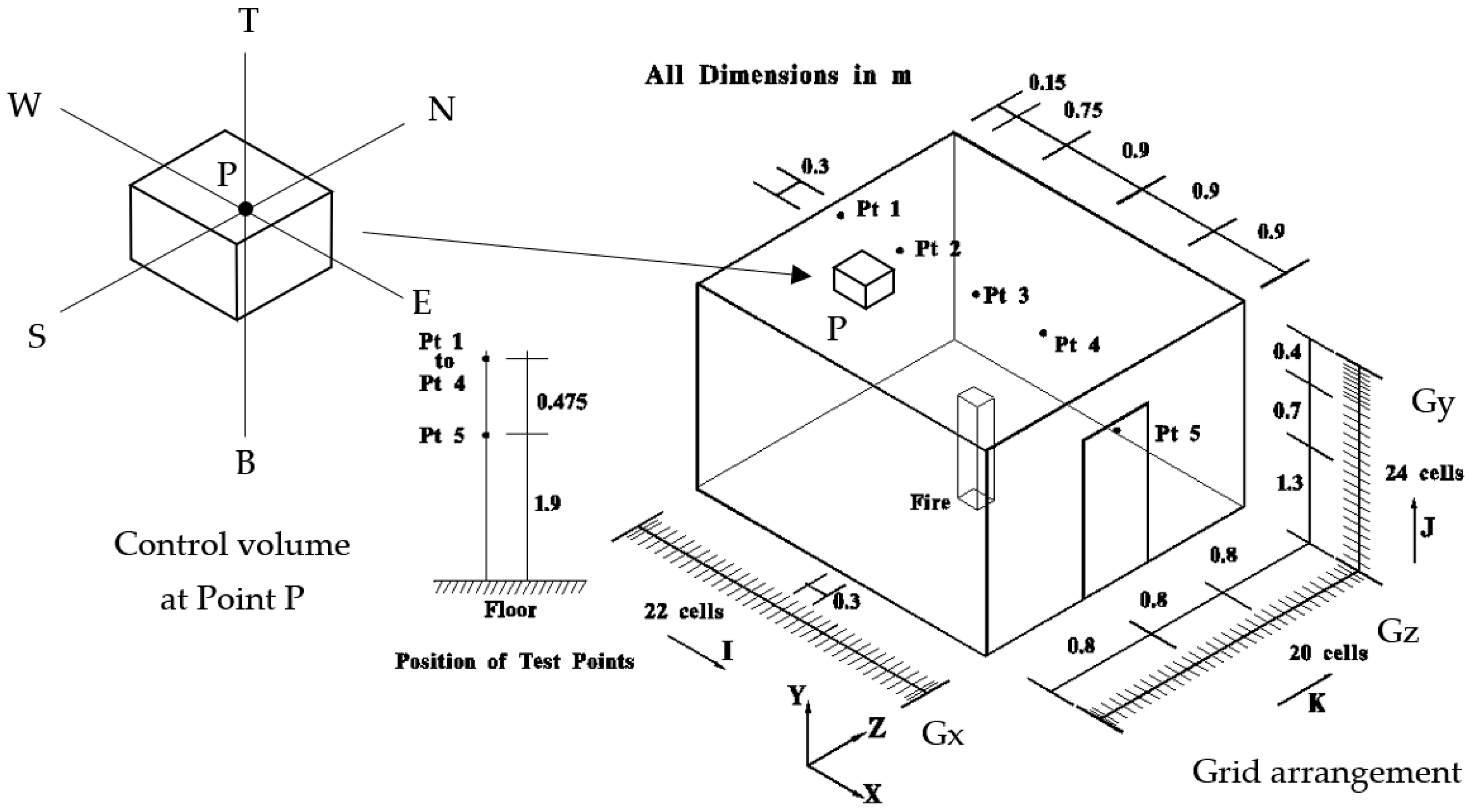There are eight variables to be solved, i.e., the three velocity components u, v, and w (using a Cartesian co-ordinate system in terms of x, y, and z, referring to Figure 1), air pressure p, enthalpy h, smoke concentration f, turbulent kinetic energy k, and its dissipation rate ε. Except for pressure, these variables are described by conservation laws which appear in a similar form. Assuming the variable ϕ stands for any one of the seven fluid variables, the equation for ϕ is

$$\frac{\partial (\rho \varphi )}{\partial t}+div[\rho \overline{V}\varphi -J_{\varphi }]=S_{\varphi }$$

(1)

The variables $\rho$, $\overline{V}$, $J_{\varphi }$, and $S_{\varphi }$ are the density, velocity vector (with co-ordinate system referring to Figure 1), diffusive flux vector, and source rate per unit volume, respectively. The velocity $\overline{V}$ and diffusive flux $J_{\varphi }$ are given by

$$\overline{V}=u\hat{x}+v\hat{y}+w\hat{z}$$

(2)

$$J_{\varphi }=-{\mathsf{\Gamma }}_{\varphi }grad\varphi$$

(3)

where ${\mathsf{\Gamma }}_{\varphi }$ denotes the effective exchange coefficient of ϕ and is determined from the turbulence parameters k and ε.

The above equations are generally applied to describe the instantaneous state of the turbulent fire field. However, in an engineering application, the average behaviour of the turbulent fire field is of more interest. Emphasis is therefore put on the mean flow behaviours rather than the instantaneous properties of flow. Any instantaneous value of those air flow variables ${\varphi }_t$ (e.g., air velocity, pressure, and enthalpy) can be expressed as its average value ϕ plus its fluctuation ${\varphi }^{\prime }$:

$${\varphi }_t=\varphi +{\varphi }^{\prime }$$

(4)

Similarly, the time averaging of Equation (1) gives:

$$\begin{array}{c}\frac{\partial \left(\rho \varphi \right)}{\partial }+div\left[\rho \overline{V}\varphi -J_{\varphi }\right]=\left[-\frac{\partial \rho \overline{u^{\prime }{\varphi }^{\prime }}}{\partial x}-\frac{\partial \rho \overline{v^{\prime }{\varphi }^{\prime }}}{\partial y}-\frac{\partial \rho \overline{w^{\prime }{\varphi }^{\prime }}}{\partial z}\right]+S_{\varphi }\hfill \end{array}$$

(5)

As a result, six additional unknowns, $\overline{u^{\prime }{}_i{u}^{\prime }{}_j}$, the Reynolds stresses, are obtained in the time-averaged momentum equations. Similarly, the time-averaged scalar transport equations show extra terms containing $\overline{u^{\prime }{}_i{\varphi }^{\prime }{}_{}}$. In this way, the set of equations is no longer a closed set. A turbulence model is necessary to represent the Reynolds stresses and the scalar transport terms with sufficient accuracy and generality.

3.1. Turbulence Model with Isotropic Assumption

Those turbulence models are based on the presumption that the turbulent viscosity ${\mu }_t$ is isotropic. In other words, the ratio between the Reynolds stress and the mean rate of deformation is the same in all directions.

• The standard k-ε model [2,29]:

The standard k-ε model [30] has two model equations, one for k and one for ε. The effective viscosity μ_eff due to turbulence is expressed in terms of two turbulence parameters k and ε, as:

$${\mu }_{eff}={\mu }_l+\frac{0.09\rho k^2}{\epsilon }$$

(6)

These turbulence parameters have to be solved by two additional transport equations on k and ε, with empirical constants C₁, C₂, and C_D:

• Low Reynolds number (LRN) k-ε model [26,30,31,32]:

The k-ε model was extended by Jones and Launder [31] to low Reynolds numbers so that the turbulence model equations can be valid throughout the laminar, transition, and fully turbulent regions. The effective viscosity μ_eff due to turbulence is expressed in terms of two turbulence parameters k and ε, as:

$${\mu }_{eff}={\mu }_l+\frac{C_{\mu }\rho k^2}{\epsilon }$$

(7)

In these equations, most of the constants retain the values assigned to them for high Reynolds numbers while C₂ and C_μ vary with the turbulence Reynolds number R_t and are shown as follows:

C_μ = C_μ∞ exp[−2.5/(1+ R_t/50)]

(8)

C₂ = C_2∞ [1 − 0.3 exp(−R_t²)]

(9)

The subscript ∞ refers to fully turbulent values. Note that the laminar diffusive transport here becomes more important in approaching the wall and the extra destruction terms included are of some significance in the viscous and transitional regions.

3.2. Turbulence Model with Non-Isotropic Treatment

• Standard k-ε model with second-order corrections [20,33]:

The k-ε model cannot produce the physical non-isotropic effects by amplifying the turbulence fluctuating in one direction and damping in the other. An algebraic Reynolds stress turbulence model can account for these non-isotropic effects. In this study, the standard k-ε model and algebraic Reynolds stress are combined to form a hybrid to account for the non-isotropic turbulence due to buoyancy. The theories of the algebraic Reynolds stress model were well-described in the literature [20,22,26,34,35] and would not be repeated here.

Empirical parameters with appropriate assumptions are used [36,37].

• LRN k-ε model with second-order corrections [20,33]:

This is a hybrid of the k-ε model (low Reynolds) and the algebraic Reynolds stresses model. The theory behind it is similar to the hybrid of the standard k-ε model and algebraic Reynolds stresses model.

4. Numerical Methods

The set of equations given by (1) is solved by numerical methods as reported in the literature [2,5,19,29,38]. The details would not be repeated here, but a brief summary is listed. Integrating the continuity Equation (1) over the control volume as shown in Figure 1 gives:

$$a_p{\varphi }_p=a_E{\varphi }_E+a_W{\varphi }_W+a_N{\varphi }_N+a_S{\varphi }_S+a_T{\varphi }_T+a_B{\varphi }_B+b$$

(10)

$$a_E=D_{e}A\left(\left|P_e\right|\right)+\max \left(-F_e,0\right)$$

(11)

where I = E, W, N, S, T, and B; and i = e, w, n, s, t, and b.

$$a_P=a_E+a_W+a_N+a_S+a_T+a_B+{\rho }^o\frac{\mathsf{\Delta }V}{\mathsf{\Delta }t}-S_P\mathsf{\Delta }V$$

(12)

$$b=S_C\mathsf{\Delta }V+\frac{{\rho }_p^o{\varphi }_P^o\mathsf{\Delta }V}{\mathsf{\Delta }t}$$

(13)

The power law scheme is used:

$$A\left(\left|P\right|\right)=\max \left(0,{\left(1-0.1\left|P\right|\right)}^5\right)$$

(14)

The discretization equation relates the global value of ϕ at the node P to its immediate neighbouring nodes E, W, N, S, T, and B with local production terms. The coefficients $a_P$, $a_E$, $a_W$, $a_N$, $a_S$, $a_T$, and $a_B$ reflect the contributions from distinct nodes due to the convective and diffusive transport of ϕ along the direction joining with the node P the neighbours E, W, N, S, T, and B. The equations are solved using the Semi-Implicit Method for Pressure-Linked Equation Revised (SIMPLER).

The accuracy of the solutions of the differential equations is strongly influenced by the boundary conditions. Therefore, the treatment of the boundary conditions, especially for solid walls, should be considered carefully. There are two types of boundary conditions used: solid wall boundary and free boundary. A summary is listed in

Table 1. Summary of the boundary conditions.

	k-ε Models and Its Modifications
Momentum equation u, v, and w
Free boundary:	$\frac{\partial u}{\partial x}=0$, $\frac{\partial v}{\partial y}=0$, $\frac{\partial w}{\partial z}=0$
Solid boundary:	Velocity components normal to the solid wall are set to be zero.
Enthalpy equation h
Free boundary:	$\frac{\partial h_x}{\partial x}=0$, $\frac{\partial h_y}{\partial y}=0$, $\frac{\partial h_z}{\partial z}=0$
Solid boundary:	For adiabatic case, $h_{flux}=0$
Turbulent parameter:
k-equation
Free boundary:	$\frac{\partial k}{\partial x}=0$
Solid boundary:	$G_k=\frac{{\tau }_s{u}_p}{y_p}$, ${\tau }_s=\frac{0.42\times y^{+}}{In\left(E{y}^{+}\right)}$
ε-equation
Free boundary:	$\frac{\partial \epsilon }{\partial x}=0$
Solid boundary:	${\epsilon }_p=\frac{C_d^{3/4}{k}_p^{3/2}}{k{y}_p}$

.

For the enthalpy equation, an adiabatic wall condition is assumed for the solid wall. The convective heat flux through the interior wall ($h_{flux}$) is equal to zero. The local convection and diffusion of turbulent energy at a wall are assumed to be negligible. There is no flux contributed from the wall. The flux expression for k is suppressed by setting the coefficient $a_s$ at the solid wall to be zero. The generation term $G_k$ for $k_p$ on the solid wall can be evaluated using the expression listed in Table 1.

The modified generation term is then incorporated into the source term of the k equation to solve for $k_p$ at the wall boundary. The treatment of k and ε at the free boundary is similar to the enthalpy equation.

5. Numerical Experiments

A series of experiments had been carried out to study the fire-induced air flow in a test compartment [39] for providing experimental data to validate the field models. The data are now used in the present study for validating the computed results by using the zonal turbulence model.

The geometrical configuration of the chamber used in the numerical study was of length 3.6 m, width 2.4 m, and height 2.4 m as shown in Figure 1. A fire of size 0.117 m³ was located at the corner of the chamber. The heat release rate followed the experimental result from the Fire Test of University of Canterbury. The heat release rate was set to be increased from 0 to 55 kW in 50 s. Four thermocouples were placed at the compartment ceiling on the vertical mid-plane to study the variation of the temperature and one thermocouple was placed on the top of the doorway.

The chamber is divided into a coarse grid system of 22 × 24 × 20 cells along the directions x, y, and z, respectively, as shown in Figure 1. The grid boundary along each x, y, and z direction are shown in lines Gx, Gy, and Gz in the figure. Note that the y co-ordinate is taken to be the vertical direction. For a better simulation, the grid sizes are not uniform. The fire source and some critical locations are modeled with smaller grids. The locations of the monitoring points are shown clearly. A personal computer notebook can be used for the simulation. The time step was 0.1 s. The convergence criterion for solving all flow variables ϕ is:

$$R_{\varphi }={\displaystyle \sum \left|R_p\right|}<R_{ref}$$

(15)

where $R_{ref}$ is a chosen value and $R_{\varphi }$ represents the sum of the absolute residual errors for any variable ϕ. This condition must be satisfied before marching to the next time step. If $R_p$ <1 for all grid points, then the program can go to the next time step.

6. Development of Zonal Turbulence Model

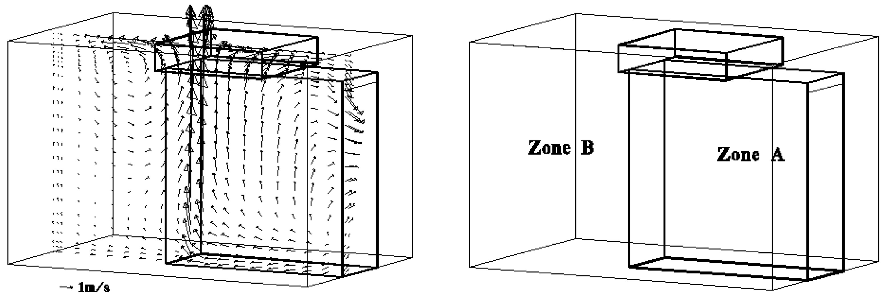
In accordance with the zonal turbulence methodology outlined in Section 2, the fire-induced flow is first computed with the base turbulence model, i.e., the standard k-ε model. The flow field is presented in Figure 2, and the three distinct flow regions—fire plume region, flow entrainment region, and recirculating region—are clearly identified. For the sake of simplicity, two zones are addressed as Zone A and Zone B. The flow in Zone A, the fire plume and entrainment regions are classified as a region with high mean-flow Reynolds numbers, and isotropic (non-directional), whereas the flow characteristic of Zone B, the recirculating region, is anisotropic (directional) with a relatively low Reynolds number. The cells of Zone A are I: 9 to 23, J: 2 to 20, K: 9 to 14, and I: 9 to 16, J: 21 to 25, K: 7 to 16. The rest of the cells belong to Zone B.

Based on the specific properties of Zone A and B, modifications of the base turbulence model can be applied, respectively. The theories behind this have already been explained in Section 3, and are shown as follows:

• Zone A: A high mean-flow Reynolds numbers and isotropic (directional) region where the standard k-ε model was applied.
• Zone B: A relatively low mean-flow Reynolds numbers and anisotropic (non-directional) region where the standard k-ε model and LRN k-ε model with second-order corrections were applied.

The following two combinations of turbulence models were tested while using the zonal turbulence modeling:

(a)

Tu 2: Standard k-ε model and standard k-ε model with second-order corrections;

(b)

Tu 3: Standard k-ε model and LRN k-ε model with second-order corrections.

7. Results

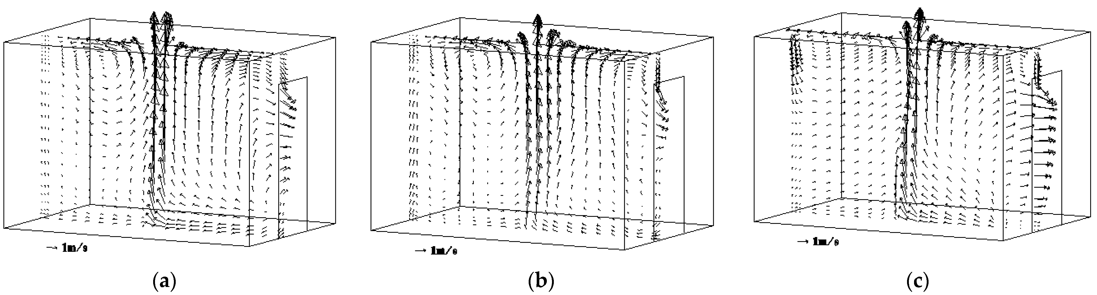
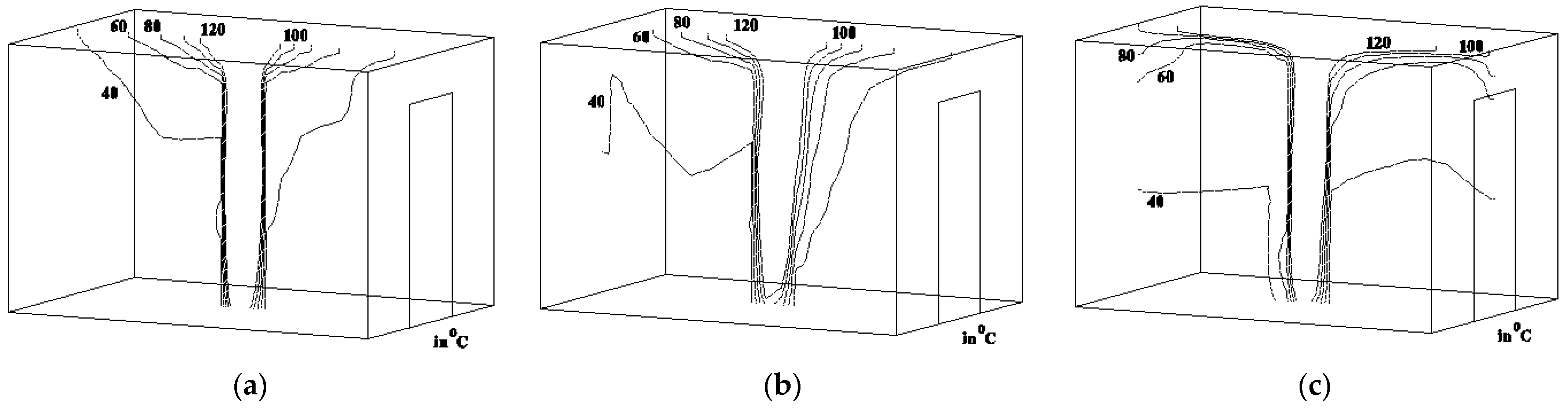
The predicted velocity and temperature fields on the vertical plane, k = 11, of the compartment at 100 s after starting the fire are calculated. Those predictions using the k-ε model and two different combinations of zonal turbulence models are shown in Figure 3 and Figure 4.

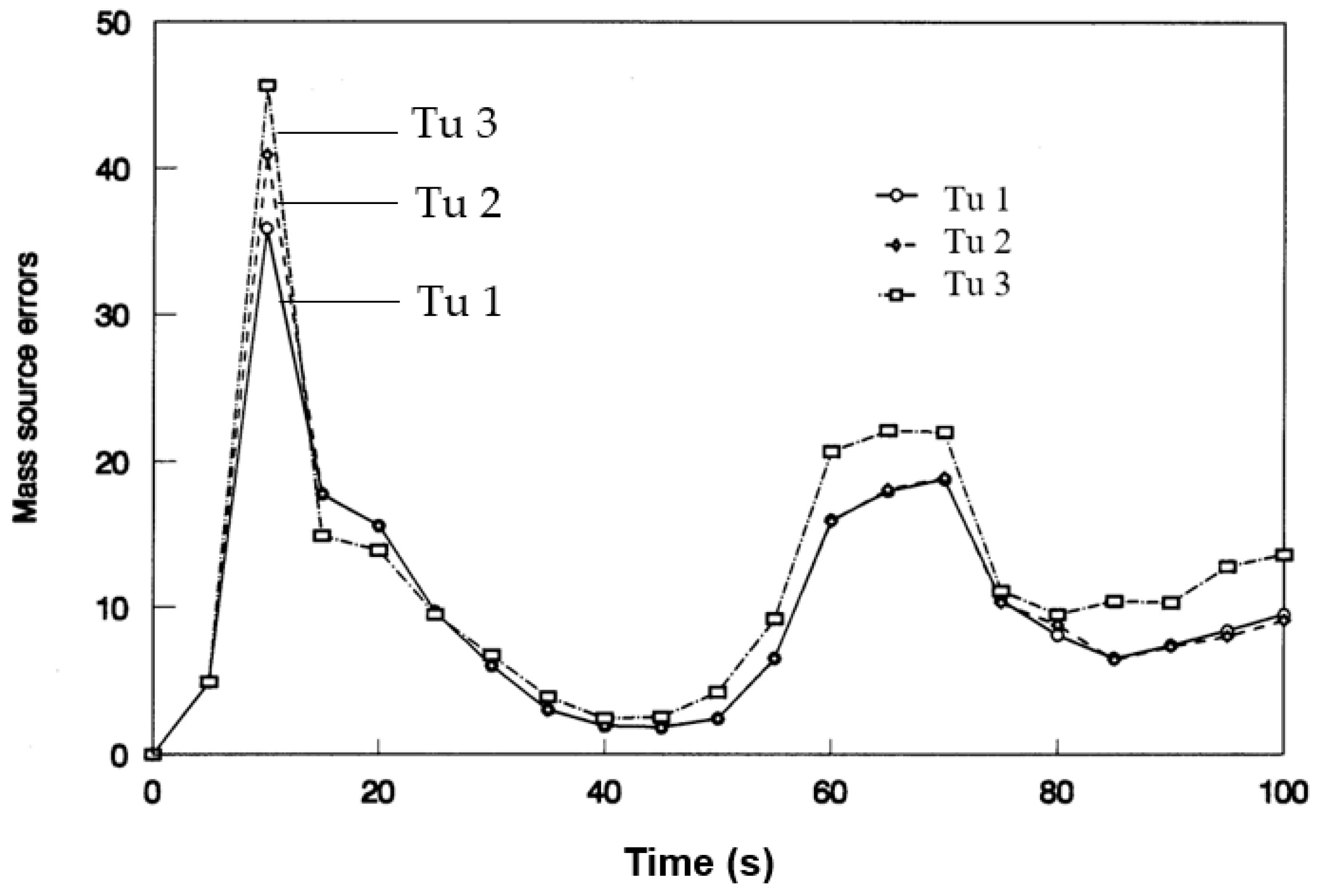
The mass source error is defined as:

$$\mathrm{Mass} \mathrm{source} \mathrm{error}={\displaystyle \sum \left|\frac{\mathsf{\Delta }p}{\mathsf{\Delta }t}+\frac{\mathsf{\Delta }(\rho u)}{\mathsf{\Delta }x}+\frac{\mathsf{\Delta }(\rho v)}{\mathsf{\Delta }y}+\frac{\mathsf{\Delta }(\rho w)}{\mathsf{\Delta }z}\right|}$$

(16)

The mass source errors at 100 s for Tu 1, Tu 2, and Tu 3 are 9.5, 9.1, and 13.6, respectively. Higher mass sources are expected because combustion is not simulated. The turbulent flow was still under transition. The transient values are plotted in Figure 5.

The percent deviation PD is given by:

$$\mathrm{PD}=\left|({\varphi }_{SIM}-{\varphi }_{Tu1}\right.)/\left.{\varphi }_{Tu1})\right|\times 100\%$$

(17)

The percentage deviation with respect to Tu 1 or Tu 2 is 4.2%, and 43.2% for Tu 3.

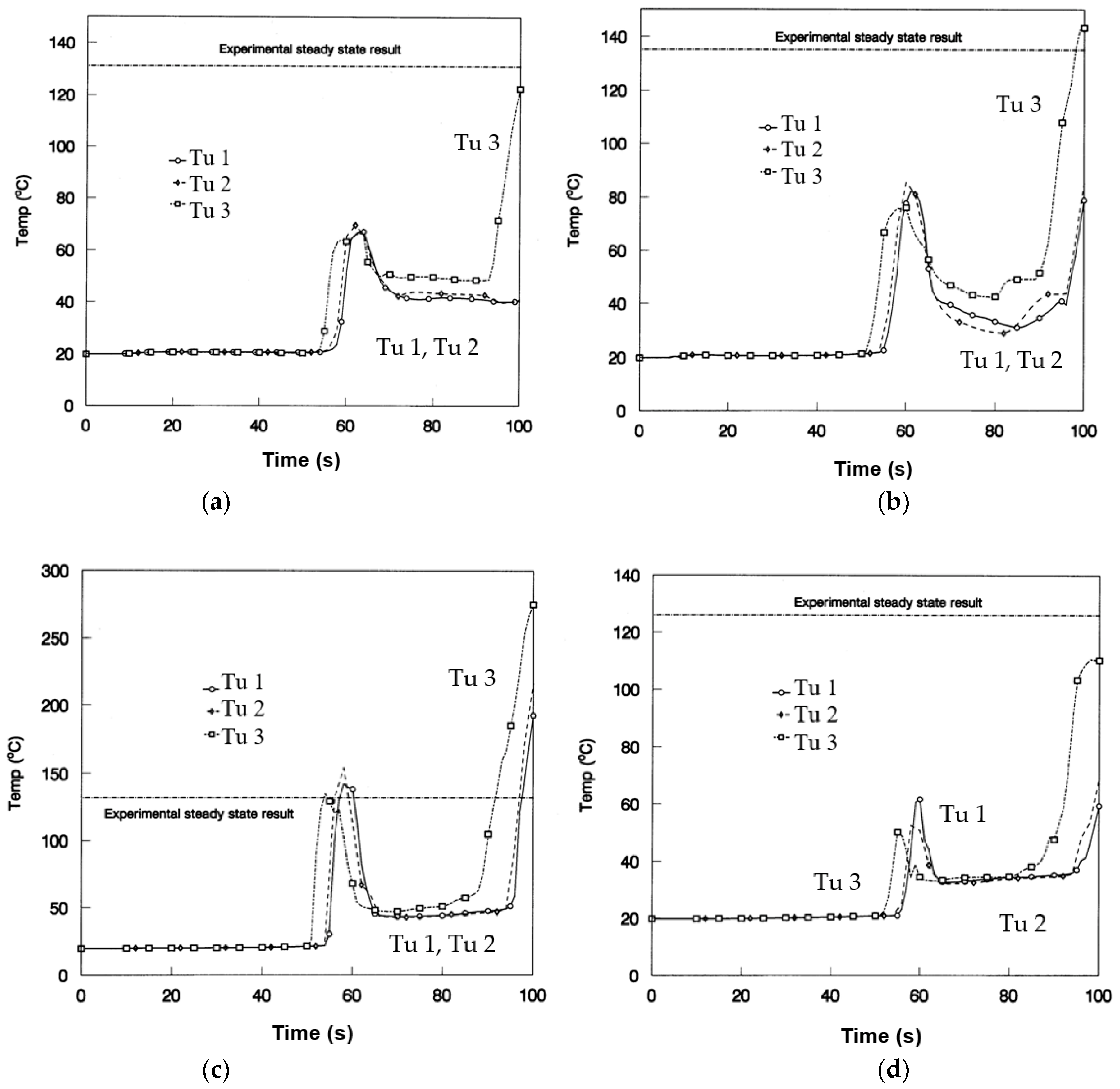
The predicted transient temperature for the various monitoring points Pt1 to Pt5 are shown in Figure 6a–e, and the numerical values are shown in

Table 2. Comparison of experimental and simulated results of temperature at 100 s.

	Temp °C
Pt	Measured	Tu 1	Tu 2	Tu 3
	Value	k-ε Model	k-ε Model + k-ε Model with Second-Order Correction	k-ε Model + LRN k-ε Model with Second-Order Correction
1	131	40.8 (68.8%)	40.3 (69.3%)	122.5 (6.5%)
2	135.1	78.8 (41.7%)	85.2 (36.9%)	143.4 (6.2%)
3	132	192.4 (45.8%)	216.3 (63.9%)	274.5 (108%)
4	126	59.3 (52.9%)	69.1 (45.2%)	110.3 (12.5%)
5	117.5	31 (73.6%)	31 (73.6%)	53.2 (54.7%)

Values in parentheses are percent deviation, = $\left|({\varphi }_{SIM}-{\varphi }_{MEA}\right.)/\left.{\varphi }_{MEA})\right|\times 100\%$.

. The CPU time required for running the various turbulence models is roughly the same of less than 5 h in the notebook.

From the computed data of Pt 3, it is observed that there are significant differences between the measured and simulated results as illustrated in Table 2 and Figure 6. Pt 3 was located at the ceiling right above the fire source which was highly affected by the feature of the heat source. The fire was described by a volumetric heat source that did not quite match a real fire with combustion reactions modelled [28]. There are thousands of intermediate reactions in the burning process; such discrepancy is expected for simulations without a combustion model. Including a realistic combustion model might improve the results. In addition, this study is focused on the comparison of different turbulence models rather than the spread of fire.

When comparing the results of the standard k-ε model (Tu 1) and the zonal turbulence model (Tu 2), which is a combination of the standard k-ε model and the standard k-ε model with a second-order correction, Tu 2 provided overall better predictions of temperature. At monitoring points Pt 1 and Pt 5, similar results were predicted by both turbulence models. However, at monitoring points Pt 2 and Pt 4, better predictions of temperature by Tu 2 were recorded with an improvement of up to 4.8% and 7.7%, respectively, compared to Tu 1. From the predicted flow field as shown in Figure 3, the recirculating regions located at both the left and right top corners were found to be more developed in the simulation of Tu 2 than Tu 1. It can be one of the reasons for the improvement of the simulated temperature at monitoring points Pt 2 and Pt 4 by Tu 2. By studying the predicted temperature fields in Figure 4, it was observed that temperature layers were developed in the simulation of Tu 2. Regarding the mass source error, both turbulence models Tu 1 and Tu 2 provided reasonable and stable values, which were recorded as 9.5 and 9.1, respectively, at time 100 s. The required CPU time for Tu 1 was 4.5 h and Tu 2 took 4.72 h to complete the program. The difference was small at only about 4.9%. It can be seen that the standard k-ε model and standard k-ε model with a second-order correction (Tu 2) provided more accurate results with only marginally more computational effort than the standard k-ε model. It has been explained [20] that the second-order correction is merely the redistribution of the turbulent kinetic energy between the x-, y-, and z-directions. The ASM corrections of the normal Reynolds stresses do not affect the total turbulent kinetic energy, since their sum equals zero [20]. The contribution ($\overline{u_i^{\prime }{u}_j^{\prime }}$)_ASM to the total Reynolds stress can be seen as a linear uncoupled ASM correction to the standard k-ε model.

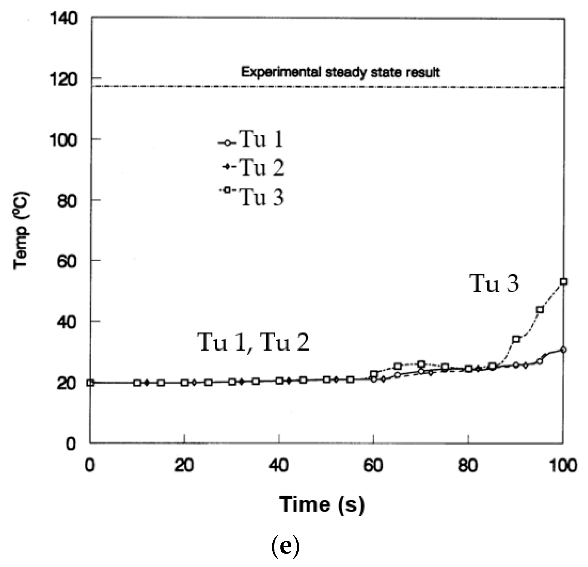
From the comparison between the standard k-ε model (Tu 1) and the zonal turbulence model (Tu 3), which is the combination of the standard k-ε model and the LRN k-ε model with a second-order correction, Tu 3 showed a significant improvement in the prediction of temperature. At monitoring point Pt 1 on the left top corner of the compartment, the simulated temperature by Tu 1 and Tu 3 were 40.8 °C and 122.5 °C, respectively, and the measured temperature was 131 °C. The improvement made by Tu 3 was about 62.3% better than the result by Tu 1. When studying the results at Pt 2, the percentage deviations from the experiment on the average simulated temperature predicted by Tu 1 and Tu 3 were about 41.7% and 6.2%, respectively. The recorded improvement was about 35.5%. From the predicted flow fields as shown in Figure 3, the recirculating flow was developed up to the left wall and the mixing of the flow was extensive in the simulation of Tu 3, whereas the development of the recirculating flow by Tu 1 was confined. As a result, the temperature predicted by Tu 3 was better than Tu 1. Similarly, Tu 3 performed better than Tu 1 at Pt 4 with up to a 40.4% improvement. The simulated temperature by Tu 1 and Tu 3 were 59.3 °C and 110.3 °C, respectively, and the measured temperature was 126 °C.

At Pt 5, it can be seen that there are significant differences between the measured and simulated results by all three turbulence models. One possible explanation is that the monitoring location of Pt 5 is very close to the computational boundaries, where the accuracy of the boundary conditions specified would affect the predicted results. Accurate measurements on the free boundaries may improve the simulated results and are recommended for further studies.

From Tu 1 and Tu 3, the simulated data were 31 °C and 53.2 °C, respectively at Pt 5. By comparing with the measured temperature at Pt 5, the deviations were 73.6% for Tu 1 and 53.2% for Tu 3. Although the results by both models had a rather great discrepancy with the experimental results, it was clear that Tu 3 provided better predictions than Tu 1 with up to about a 20.4% improvement.

With respect to the flow field shown in Figure 3, the recirculating regions by Tu 3 extensively developed at the top corners of the compartment; a significant improvement was observed when comparing with Tu 1 or even Tu 2. By studying the predicted temperature field in Figure 4, Tu 3 provided a temperature field with a more sophisticated development of temperature layers. The results were also in line with the theory [20,26,30] that the LRN k-ε model can better handle the viscous effects in the viscous sub-layers near the walls than the standard k-ε model. Regarding the mass source error, the pattern of the transient values of Tu 3 was similar to Tu 2, as they were applying the same base model turbulence model, k-ε model, with modifications. At time 100 s, the mass source error of Tu 3 was 13.6 or 43.2% more compared to Tu 1 and this can be explained by the theory [18,20,26,30] behind Tu 3, for which a relatively more complicated turbulence model was applied. In addition, the value was found to be well within the reasonable and acceptable level. The required CPU time for Tu 3 was 5.02 h or 11.56% longer than Tu 1, but up to a 62.8% (at Pt 1) improvement in predicting temperature.

8. Boundary of the Flow Regions

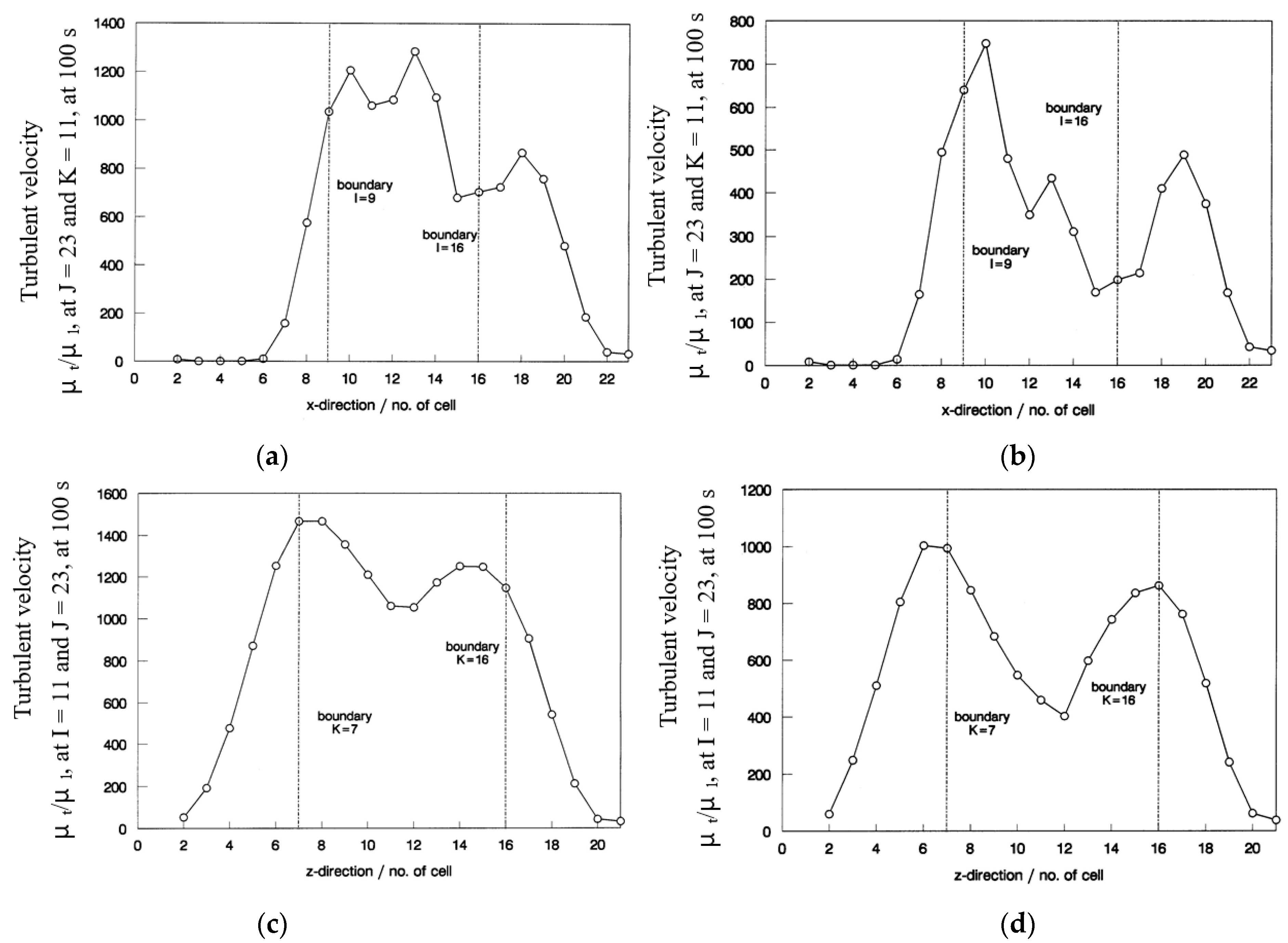
As mentioned in Section 2, the discontinuity problem is one of the major difficulties of the zonal turbulence model. For the two cases of zonal turbulence models, Tu 2 and Tu 3, the turbulent-viscosity-to-laminar-viscosity ratio ((${\mu }_t/{\mu }_l$) was inspected to check the continuity.

The viscosity ratio (${\mu }_t/{\mu }_l$) along the x-axis for J = 23 and K = 11 by Tu 2 and Tu 3 were plotted in Figure 7a,c. The variations of viscosity ratio (${\mu }_t/{\mu }_l$) along the z-axis for I = 11 and J = 23 by Tu 2 and Tu 3 are shown in Figure 7b,d.

From the data, no significant discontinuity was recorded. The gradients $\frac{d\left({\mu }_t/{\mu }_l\right)}{dx}$ and $\frac{d\left({\mu }_t/{\mu }_l\right)}{dy}$ for the ratio ((${\mu }_t/{\mu }_l$) across the boundary by Tu 2 were 850 m⁻¹ at I = 9, 100 m⁻¹ at I = 16, 2140 m⁻¹ at K = 7, and −2410 m⁻¹ at K = 16. Similarly, the gradients across the boundary by Tu 3 were 540 m⁻¹ at I = 9, 80 m⁻¹ at I = 16, −90 m⁻¹ at K = 7, and −1020 m⁻¹ at K = 16.

This is only a qualitative comparison of the zonal turbulence model. Further studies with experiments are needed on the boundary phenomenon.

9. Conclusions

Fire-induced flow in a compartment has been computed with the standard k-ε model first (Tu 1). Based on the computed flow field, different regions with distinct turbulence features are located and suitable modifications of the standard k-ε model are proposed. By combining different modifications of the standard k-ε model targeted on different regions, two zonal turbulence models are formed, which are Tu 2 (standard k-ε model and standard k-ε model with a second-order correction) and Tu 3 (standard k-ε model and LRN k-ε model with a second-order correction).

The results indicate that the zonal models provide superior predictions for most of the zones in the flow field when compared to the standard k-ε model. The improvements will be varied according to the suitability of the modifications of the k-ε model applied in specific zones. Moreover, one of the major problems in zonal turbulence modeling is the discontinuity across the boundary of different zones. In this study, a solution is proposed by using similar types of turbulence models, i.e., the k-ε model and its modifications, and reasonable results were obtained. However, the selections of turbulence models for combination are limited. Further research in the combination of different turbulence models is required.

The zonal turbulence modeling approach proposed above is appropriate for carrying out a high number of simulations in a preliminary study on identifying typical scenarios in initial hazard assessments while applying a performance-based design. This will give a reasonable accuracy within affordable computing resources. The identified scenarios can then be studied more thoroughly using a much smaller number of LES simulations and confirmed by previous full-scale burning tests. The cost of hazard assessments on compartment fires is then highly reduced.