1. Introduction
In tokamaks, a few percent of plasma current pulses can terminate uncontrollably in the form of either major disruptions (MDs) or vertical displacement events, which may be symmetric or asymmetric (VDEs or AVDEs, respectively), e.g., [
1,
2,
3,
4,
5,
6,
7]. A common feature of MDs, VDEs, and AVDEs is that they all conclude with the termination of plasma current. This distinguishes them from other typically more rapid or less intensive plasma events, such as various instabilities and thermal quench (“TQ”). TQ is a quick phase within MDs, VDEs, or AVDEs. This article concentrates on the calculation of EM loads acting on tokamak components at VDEs and AVDEs.
For ITER-scale tokamaks, the duration of plasma current decay (current quench, “CQ”) during MDs, VDEs, or AVDEs ranges from a few tens to a few hundreds of milliseconds. Since plasma current finally terminates, the distortions of the electromagnetic (EM) field always have enough time to penetrate through the vacuum vessel (“VV”) and, accordingly, always cause EM interaction between the VV and the tokamak coil system (“the Magnets”). Even when the plasma current vanishes, a significant EM interaction between the VV and the Magnets remains as long as the VV carries eddy currents. Characteristic ramp-up times for these EM loads correlate with the rate of penetration of the magnetic field distortions through VV walls. The transient field penetrates not with the decay time of net toroidal current in the VV (~1 s for ITER) but with decay times of eddy currents in the higher modes (quadruple, saddle, and many local modes). The higher modes have shorter characteristic times; thus, EM loads between the VV and the Magnets start growing rather early. If an MD or VDE occurs with a rather short CQ phase, EM loads between the VV and the Magnets reach their extremes when the plasma current has already terminated. For VDEs or AVDEs occurring with relatively longer CQ time, some components of EM loads reach their extremes during the CQ phase, while other load components do peak after plasma termination. Proof can be seen in patterns of currents in the VV, in graphs of coil currents delivered by plasma evolution codes, e.g., [
1,
2,
8,
9,
10], or in graphs of net EM loads acting on the VV and the Magnets obtained with detailed EM post-processing models, e.g., [
11,
12,
13], as well as in this article. The above explanation for a rather early EM interaction between the VV and the Magnets was highlighted by one of the authors of this paper a long time ago in a course of VDE simulations on 2D and 2.5D tokamak models [
1]. We reiterate it here since it helps to understand the basis of the presented approach. It is hard to find in modern publications, although it is mentioned in [
5,
14].
To summarize, the practical EM model described herein was developed for the calculation of AVDE-induced EM loads acting on the VV and the Magnets, with the plasma behaving as a massless link between these two. We do not consider any “rapid” plasma events, which evolve faster than the decay times of higher modes of VV eddy currents and avoid the termination of plasma current because they cause modest or negligible net loads from EM interaction between the VV and the Magnets.
Some plasma evolution codes, e.g., [
1,
8,
9,
10], can operate in the following two modes: (a) for the synthesis of coil current waveforms needed for normal operational pulses and (b) for the simulation of uncontrolled plasma evolution and resultant EM transients during MDs and VDEs. Papers [
8,
9], describing the well-known code DINA, use the term “scenario” for both these meanings. Our EM model employs, as a part of its inputs, one of the VDE evolution scenarios delivered by the code DINA and stored in the “ITER DINA library”.
Typically, MD or VDE scenarios delivered by a trusted plasma simulation code serve then as inputs for 3D post-processing with specialized EM codes, e.g., [
11,
12,
13]. The latter produces detailed time-dependent maps of eddy currents and EM force densities for all major tokamak systems as a basis for further engineering analyses. Results provided by various EM analysis teams in terms of axially symmetric components of pulsed EM loads during MDs and VDEs usually have a good mutual agreement and thus are not discussed here. We concentrate instead on the calculation of lateral vectors of AVDE-induced EM loads.
It is well-known that a tokamak is a practically closed EM system. This is trivial for analytical considerations; however, it is not always easy to obey with complex numerical EM models. In principle, any numerical model used for the calculation of EM loads in all major tokamak systems during MDs, VDEs, and AVDEs always delivers well-compensated EM loads with practically zero net force and moment for both the plasma and the entire tokamak. However, all numerical models are not ideal, and accurate enough numerical implementation of this generic conservation law with complex 3D models for EM transients in the entire tokamak is not always enforced as it should. A scale of residual numerical mismatches, definitively requiring compensation, can be seen in
Section 5. This is why such trivial criteria should be carefully tracked in calculations of EM loads on complex 3D models and clearly demonstrated in numerical outputs. In rather old VDE simulations [
1], net EM force balance and total EM and Joule energy in a whole tokamak were controlled well since they served as code convergence criteria. This was implemented with the involvement of one of the authors of the present paper. The necessity to control net EM load balance in outputs of complex 3D models is reiterated explicitly in [
14] and implemented carefully in the present paper.
In principle, any ideally working EM model of any closed EM system (not necessarily a tokamak) will always demonstrate a net balance of EM loads. However, in practice, some residual imbalance always takes place due to the following reasons:
- (a)
The discretization of the VV is usually quite different between the two types of codes used consequently. A rather simple 2D VV model in codes providing a self-consistent simulation of plasma evolution is followed by much more complex 3D models of the VV with internal components at the EM post-processing stage.
- (b)
The unavoidable accumulation of numerical errors during the simulation of EM transients in complex 3D EM models, and then at the calculation and summation of elementary EM force vectors at the last phase of EM post-processing. Both these factors lead to quite noticeable residuals, especially for non-dominant load vectors.
For specific engineering purposes, such as the design of tokamak structures, supports, and interfaces between various components, the calculated maps of EM force densities are summed in the form of time-dependent graphs of net EM loads separately for the following two groups of tokamak components (the specific terms are for the ITER tokamak):
Everything resting on nine “VV gravity supports”, including VV shells, ribs, ports, port extensions, and all “in-vessel components”, including blanket modules, divertor cassettes, port plugs, etc.
Everything resting on 18 “toroidal field coils gravity supports”, including toroidal and poloidal field (TF and PF) coils, central solenoid (CS), etc., all composed by their superconducting windings, cases or clamps, inter-coil structures, and other “cold structures”.
In this article, we refer to these long definitions by the following shorter terms: “the VV” (or “the VV with internal components”) and “the Magnets” (or “the coils windings with cold structures”).
The reported numerical EM model has specific built-in features aimed to intrinsically obey the well-known EM load balance in a tokamak as a whole as follows:
where:
FVV—vector of the net EM force acting on the VV with all internal components;
FMg—vector of the net EM force acting on the Magnets (the windings and cold structures);
MVV—vector of the net EM moment acting on the VV with all internal components;
MMg—vector of the net EM moment acting on the Magnets (the windings and cold structures).
A reader may ask why we are not simply calculating the pulsed net EM loads at the VV only (as performed in many articles) and relying on the engineering team to apply exactly opposite waveforms of the net EM loads at the Magnets. The reasons are as follows:
- (a)
Mechanical models are fed not by net EM loads but by distributed EM loads (time-dependent maps of EM force densities), which need to be calculated specifically for each modeled component (not only for VV shells but also for blanket modules, divertor cassettes, ports and port plugs, etc., for each coil’s winding and relevant cold structures).
- (b)
The distribution of transient magnetic fields and eddy currents in the VV depends not only on plasma evolution but also on the transient EM response of the Magnets and all listed conducting structures. Thus, transient EM analysis is to be performed on the global tokamak model.
- (c)
If the EM report says nothing about transient EM loads on the Magnets, there is a risk that EM reaction loads at the Magnets will be simply omitted in a structural model.
Several tokamak physics teams, e.g., [
5,
6,
7,
15,
16,
17] and many others, are working on the experimental observation, interpretation, and consistent simulation of plasma MHD evolution during AVDEs. Our article does not intend to discuss or compare these studies. Instead, the focus is on the detailed numerical calculation of the resultant lateral EM loads acting between the VV and the Magnets. Our model calculates loads corresponding to some specific AVDE evolution scenarios, which we take as the pre-existing input assumption in a way detailed below. The two previous sentences are usually compacted in the shorter term “EM post-processing”. Thus, in short words, we offer quite a detailed and well-balanced EM model for AVDE post-processing as an upgrade of the existing EM models that served many years for MD and VDE post-processing. EM post-processing is a prerequisite for the simulation of the tokamak dynamic response to MDs, VDEs, or AVDEs with the final purpose of specifying design loads as one of the inputs for the development of tokamak’s structures and supports, blanket-to-VV and divertor-to-VV attachments, inter-coil links, and other interfaces.
Since an AVDE represents the gradually growing asymmetric distortion of the preceding VDE, this article concentrates just on the following two types of plasma events: VDEs and AVDEs.
Our EM model calculates the time-dependent distributed EM loads (maps of EM force densities) for all modeled structures and coil windings, along with the resultant six vector components of the net EM loads acting on the VV and on the Magnets. Here, we present just one set of AVDE-induced time-dependent EM loads obtained for one set of input assumptions. Later, by varying the model’s input parameters on the form and severity of AVDE distortion, we can deliver the corresponding variants of AVDE-induced EM loads. Various scenarios of AVDE evolution (serving as our inputs) may be ranked by the tokamak physics community. In this way, tokamak engineering teams could pick up “ready to use” maps of AVDE-induced EM loads, accompanied by graphs of net load vectors, for a few AVDE evolution scenarios that have been recommended as the most relevant.
We understand that it is not an easy task for the physics community to conclude with a few commonly agreed preferred scenarios of AVDE evolution. Being based on somewhat different interpretations of AVDE physics and different simplifying model assumptions, various AVDE evolution models deliver seriously diverging AVDE scenarios, and, accordingly, diverging predictions for lateral EM loads. This article’s intent is not to contribute to plasma physical interpretations, simulations, and discussions on the most likely AVDE evolution but to calculate all components of AVDE-induced EM loads for one selected input scenario. When such EM calculations are repeated with the parametric variation of inputs, this approach will gradually reveal a quantitative correlation between the assumed AVDE form and severity and the scale of the resultant lateral EM loads.
2. Common Terms and Understanding of Plasma Evolution during VDEs and AVDEs
This section recalls the most common terms and understanding of plasma evolution during VDEs and AVDEs. We relied on these for the development of the tokamak model for EM post-processing. At some stage of a VDE or an AVDE, the plasma periphery touches the first wall and forms a so-called “halo layer”. In some papers, this term also serves to describe the periphery of the detached plasma, but this is irrelevant to our model. In the halo layer, the helical plasma current intercepts the first wall or divertor panels and then flows through the conductive structures and returns to the halo layer. In other words, a loop of the halo current closes partly through the halo layer helically, and partly through the VV and in-vessel components. In terms of generic conservation laws, the halo current is driven by the compression of the toroidal magnetic flux frozen in the plasma.
Experimental data and analytical interpretations, e.g., [
5,
6,
7,
15,
16,
17], indicate that the gradual transition from a VDE to an AVDE resembles that of gradually growing kink modes. These are helical distortions that develop throughout the plasma volume but naturally have a larger scale at the plasma periphery. Phenomenological descriptions of AVDEs come in several variants. For example, ref. [
15,
16,
17] pay major attention to asymmetric helical distortions of the whole plasma before the appearance of significant halo currents. They conclude with estimates of resultant asymmetric patterns in the VV eddy currents and corresponding lateral loads at the VV. Another approach, e.g., [
13], concentrates on toroidally asymmetric loads caused by the EM interaction between the toroidal magnetic field and toroidally asymmetric halo currents only on a portion of the halo currents’ path where they flow in the VV. Toroidal asymmetry of the halo current “injected” in the VV is prescribed or reported in many papers as a “toroidal peaking factor” (“
TPF”). The
TPF is defined as the ratio of the peak-to-average linear density of halo currents entering in or exiting from the halo-to-wall interception belts.
This paper has no intention of giving an overview of a rich field of interpretations and predictions of AVDE physics. Instead, it concentrates on the calculation of time-dependent maps, graphs, and maximal net EM loads for one case of arbitrarily selected input assumptions on AVDE form and severity, as detailed in the next sections.
During each specific VDE or AVDE, plasma evolves somewhat differently because of stochastic variations in the preceding plasma state (scatter in fine details of the momentary plasma profile, shape, and position right before a VDE or an AVDE). This natural uncertainty complicates the selection of a specific “most trusted” VDE or AVDE scenario for the purposes of load specification. As a classical engineering solution in situations with naturally uncertain inputs, practical results of AVDE-induced EM loads can be obtained by a parametric study. This logic is introduced in [
18] and applied here. A parametric study means that the EM model is to be run several times at widely varied input assumptions on the form and severity of asymmetric plasma distortions. This is a practical way to quantify a correlation between (a) input assumptions of AVDE form and severity and (b) time-dependent patterns and net vectors of AVDE-induced EM loads everywhere. Being collected in a sufficient number of variants, they will fill up a kind of “AVDE load library”.
The AVDE-induced EM loads reported here were obtained to serve as the input data for the simulation of the ITER tokamak’s structural dynamic response to an AVDE, which is then used for the development of algorithms for the Tokamak Systems Monitor (“TSM”) [
19]. The development of the TSM relies on synthetic measurements acquired from numerical models. Such synthetic measurements serve as a temporary substitute for the actual sensor data, which will be available only when the ITER operates. Overall, TSM algorithms will employ measurements from a large variety of gauges and combine reconstruction and simulation techniques to deliver concise engineering information to the tokamak operator about the actual behavior and status of all tokamak systems.
This article presents specific AVDE-induced EM loads provided for the following two purposes:
- -
To populate the tokamak dynamic model as needed for the development of TSM algorithms;
- -
To offer the first practical contribution to the library of AVDE-induced EM loads.
3. Features Preserved from Previously Reported Trial EM Models
Like the trial EM models in [
18], this numerical model is built to represent the superposition of two time-dependent patterns of halo currents including (a) an axially symmetric poloidal pattern identical to the one used in VDE post-processing and (b) a perfectly anti-symmetric helical pattern built as described below.
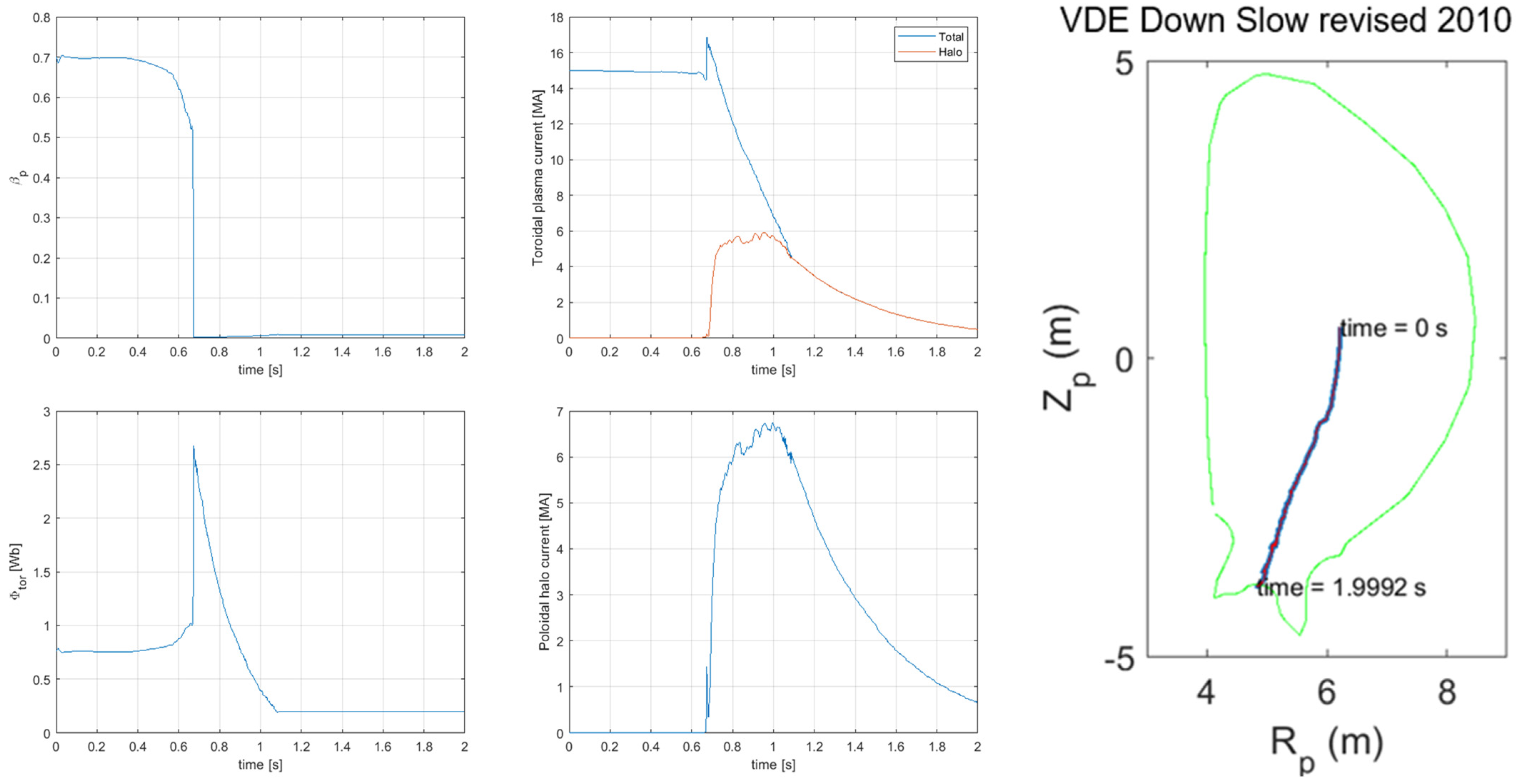
The first component, the symmetric halo current pattern, is already available as the output of any trusted code for the simulation of plasma evolution. Here, we use the pattern of the poloidal halo current for the scenario “VDE Down Slow Revised” delivered by the DINA code [
8,
9] and saved in the ITER DINA library. As is typical for VDE post-processing [
11,
12,
13], the symmetric poloidal halo current is represented by four poloidal bridges built within the 3D EM model, which is solved with the CARIDDI code [
12,
13].
The helical bridges for the anti-symmetric halo current component are then added to the numerical model to implement our specific input assumption on the scenario of AVDE evolution. The logic for the shaping of the built-in helical bridges is the following:
When VDE post-processing is performed well enough, the symmetric halo pattern:
In tokamaks with sufficiently symmetric conductive (and ferritic, if they exist) structures, the symmetric pattern of halo currents alone cannot cause significant net lateral EM loads between the VV and the Magnets. This means all components of the lateral AVDE loads (in our numerical model) are produced exclusively by the anti-symmetric halo current pattern, as detailed below.
Considering all listed balances associated with the symmetric halo pattern, the anti-symmetric halo pattern (built in our numerical model) obeys the following generic conservation laws, both on its own and after superposition with the symmetric one:
The global EM loads balance (1) is to be obeyed not only for vertical EM forces in the interaction between the VV and the Magnets but also for lateral forces and torques, meaning for all 3 + 3 = 6 orthogonal net load vectors.
Waveforms of poloidal and toroidal magnetic fluxes linked with the plasma will be preserved as they have been delivered by the plasma evolution simulation code (in our case, the DINA). This means that the anti-symmetric halo current pattern will be introduced in such a way that it remains always fully magnetically decoupled from the toroidal and poloidal magnetic fluxes produced by the plasma.
Waveforms of net vertical EM forces on the VV and the Magnets will not be disturbed but kept intact as they are derived from the symmetric VDE model. Accordingly, the anti-symmetric halo pattern itself will be built in a such way that it cannot produce net vertical EM forces in EM interaction with the VV and with the Magnets.
These three conditions for errorless superposition of two halo current patterns seriously restrict the range of shapes suitable for representation of the anti-symmetric component of the halo current as follows:
The anti-symmetric pattern will be built in such a way that its superposition with the symmetric one does not disturb any of the above-stated balances.
The last condition (after all the above-listed) is that in superposition with the symmetric pattern, the anti-symmetric one will create a pattern of plasma current density resembling one for the plasma distorted in a kink mode.
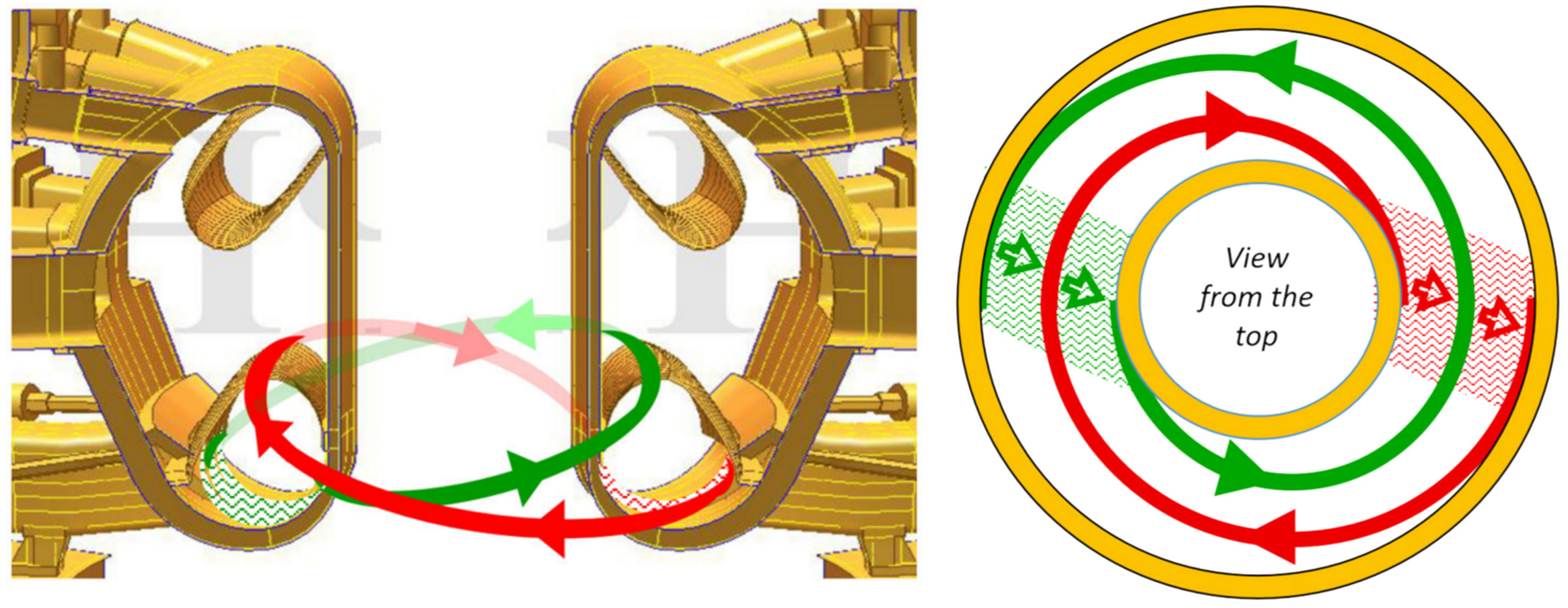
All the above-listed balances and conditions can be satisfied by upgrading the 3D EM tokamak model with the paired helical bridges visualized schematically in
Figure 1, which is copied from [
18]. For visualization purposes,
Figure 1 shows just one pair of helical bridges, while the real numerical model (
Section 4) contains 200 pairs of helical filaments. Two bridges in
Figure 1 have identical shapes but are spaced toroidally by 180 degrees and fed by opposite (“mirrored”) current waveforms. The current fed into each helical bridge forms a closed loop through the VV and in-vessel components, as shown by fuzzy red and green areas. This numerical model intrinsically obeys the continuity of electrical currents, which is not always the case in some EM calculations relying on “sink and source” halo models.
Based on experiments and AVDE interpretations described in [
5,
15,
16], we built helical bridges suited to mimic plasma current patterns in the kink mode (
m = 1;
n = 1). Later, for parametric studies, on anticipated advice of the physics community, the model may be partly re-built to mimic other helicities, e.g., (
m = 1.5;
n = 1), (
m = 2;
n = 1), etc.
To summarize, this 3D EM model works with the following input assumptions on plasma evolution during the AVDE. The time-dependent pattern of plasma current is represented as the superposition of three current patterns:
- (a)
Toroidal current in an axi-symmetric plasma core that always stays axi-symmetric during its equilibrium evolution (taken for one VDE from the ITER DINA library);
- (b)
An axi-symmetric poloidal current in the halo layer (taken from the DINA library for the same VDE case);
- (c)
A helical pattern of the anti-symmetric halo current component, which we build in the 3D model artificially, as depicted in
Figure 1, with details described in the next section.
Patterns (a) and (b) have been used previously in the same way for VDE post-processing. Pattern (c), newly built in, makes this EM model suitable for AVDE post-processing. Of course, the model has been expanded from 40 to 360 degrees, which was not realistic several years ago due to former limitations in computing power.
Of course, the AVDE post-processing input assumptions, which were previously described, mimic but do not exactly reproduce the MHD equilibrium. For example, the present EM model does not mimic Shafranov’s shift, etc. This would be a serious drawback if the purpose is to accurately simulate the evolution of MHD equilibrium during the AVDE. However, we pursue a practical task on the calculation of EM loads at the VV and the Magnets at a major event concluding by plasma termination. In this respect, the explained model simplifications seem acceptable since we intend to run this EM model with wide parametric variations of input assumptions on AVDE form and severity.
While waiting for advice on specific variants of our input assumptions from the tokamak physics community, we deliver the first example of AVDE-induced EM loads at an arbitrarily selected variant of the preceding VDE and for arbitrarily assumed form and severity of AVDE, characterized by (m = 1, n = 1), TPF = 1.5.
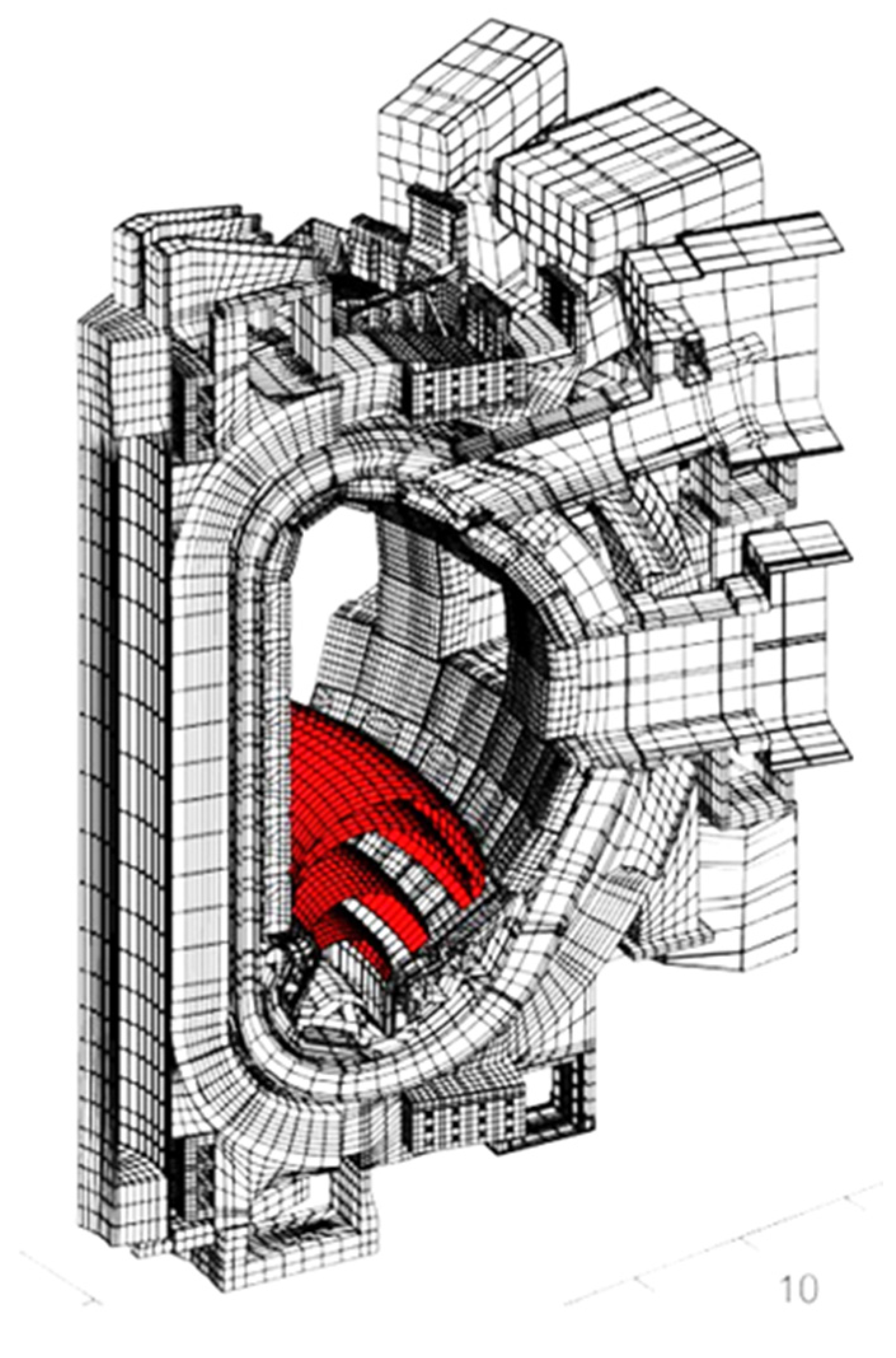
4. Details of the 3D Model Developed for the Calculation of AVDE-Induced EM Loads
The described approach is performed on a 360-degree tokamak numerical model for the EM code CARIDDI, updated from the previously used 40-degree model, e.g., [
12,
13]. The model represents the plasma current by more than a thousand toroidal, poloidal, and helical filaments, as detailed below. Each filament is fed by a specific prescribed current waveform. These elementary currents excite eddy currents in all numerically modeled tokamak structures and cause a change in currents in the windings of CS and PF coils.
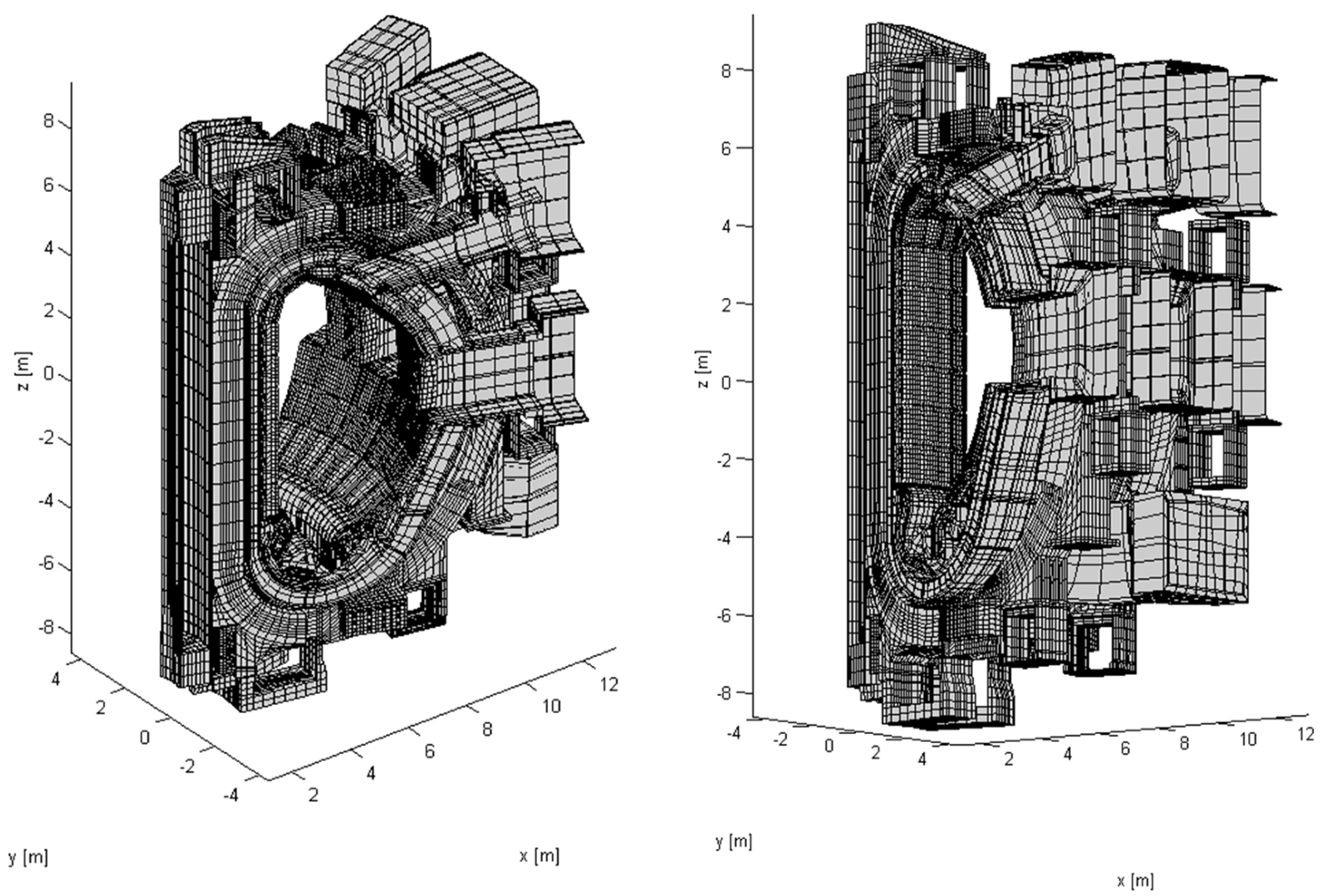
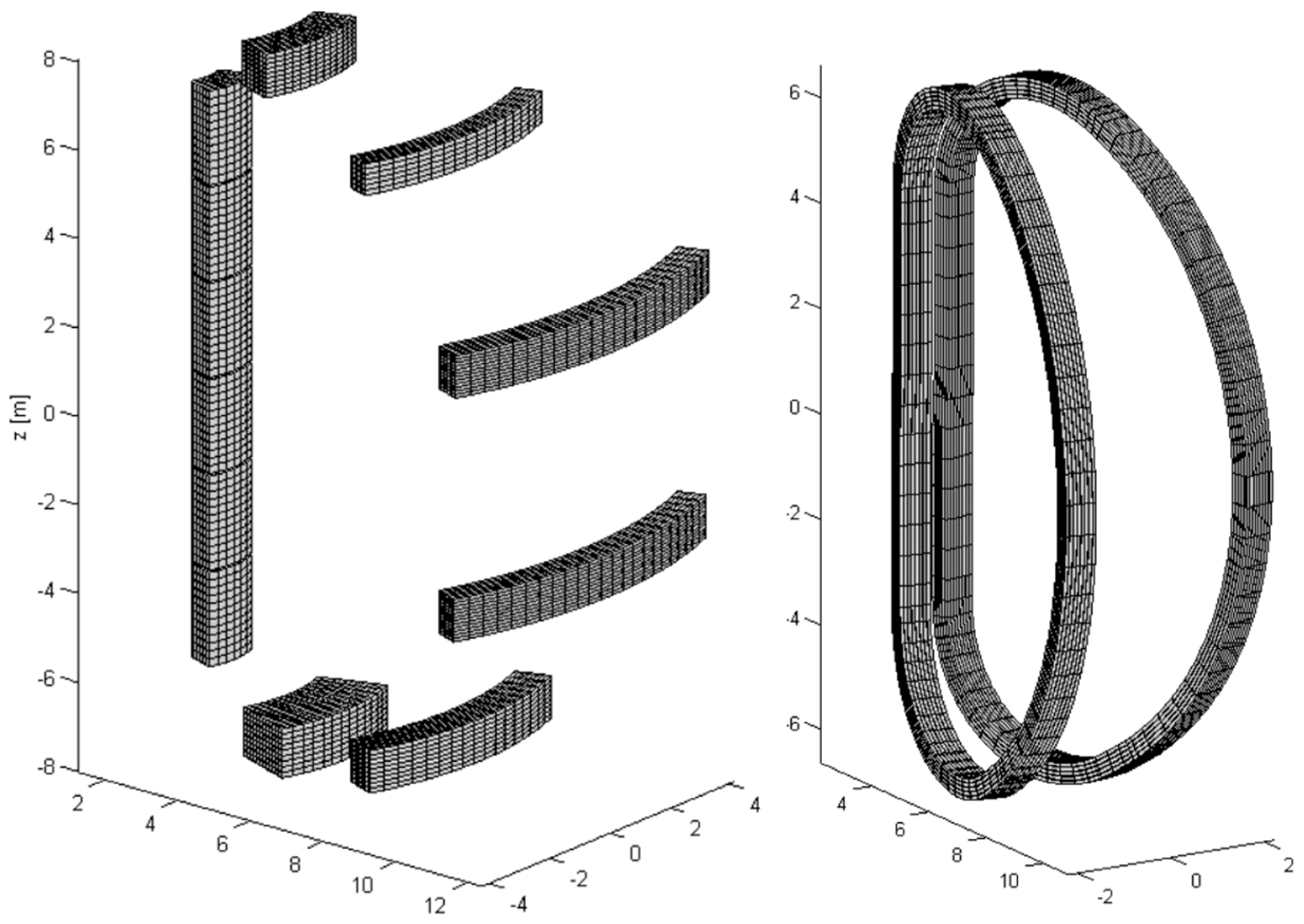
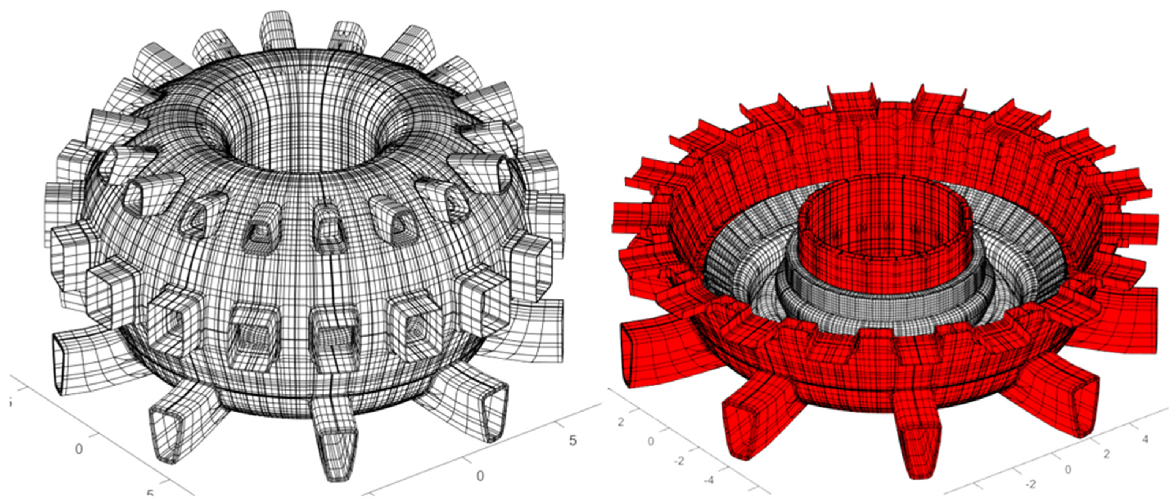
Figure 2,
Figure 3,
Figure 4 and
Figure 5 show two EM models including the pre-existing 40-degree model used for VDE post-processing and its upgrade to a 360-degree model generating AVDE-induced EM loads.
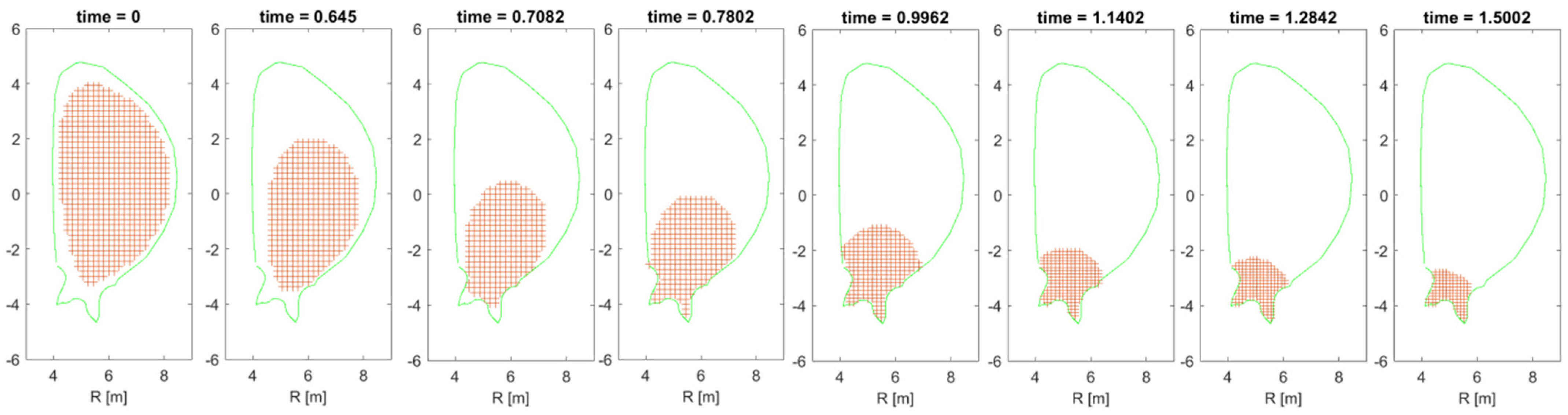
Figure 6,
Figure 7 and
Figure 8 illustrate the specific VDE scenario “VDE Down Slow revised” taken from the ITER DINA library and used initially for VDE post-processing and then for incorporation of new 3D model features as needed for the calculation of AVDE-induced EM loads.
The presented EM model for the calculation of AVDE-induced loads combines the following features of the trial AVDE models from [
18] and typical models for VDE post-processing, which have been known for a long time [
11,
12,
13]:
As per trial model #1, the present model simulates the gradual slipping of the halo current interception belts on the plasma-facing walls. It avoids the drawback of trial model #2, where halo current interception belts could not slip.
As per trial model #2, the present model simulates the halo layer wrapping around the core plasma. It avoids the drawback of trial model #1 which simulated the halo layer not wrapping around the plasma but rather inserted between the plasma and the nearest wall.
Like typical advanced VDE post-processing models [
11,
12,
13], but unlike the trial AVDE EM models [
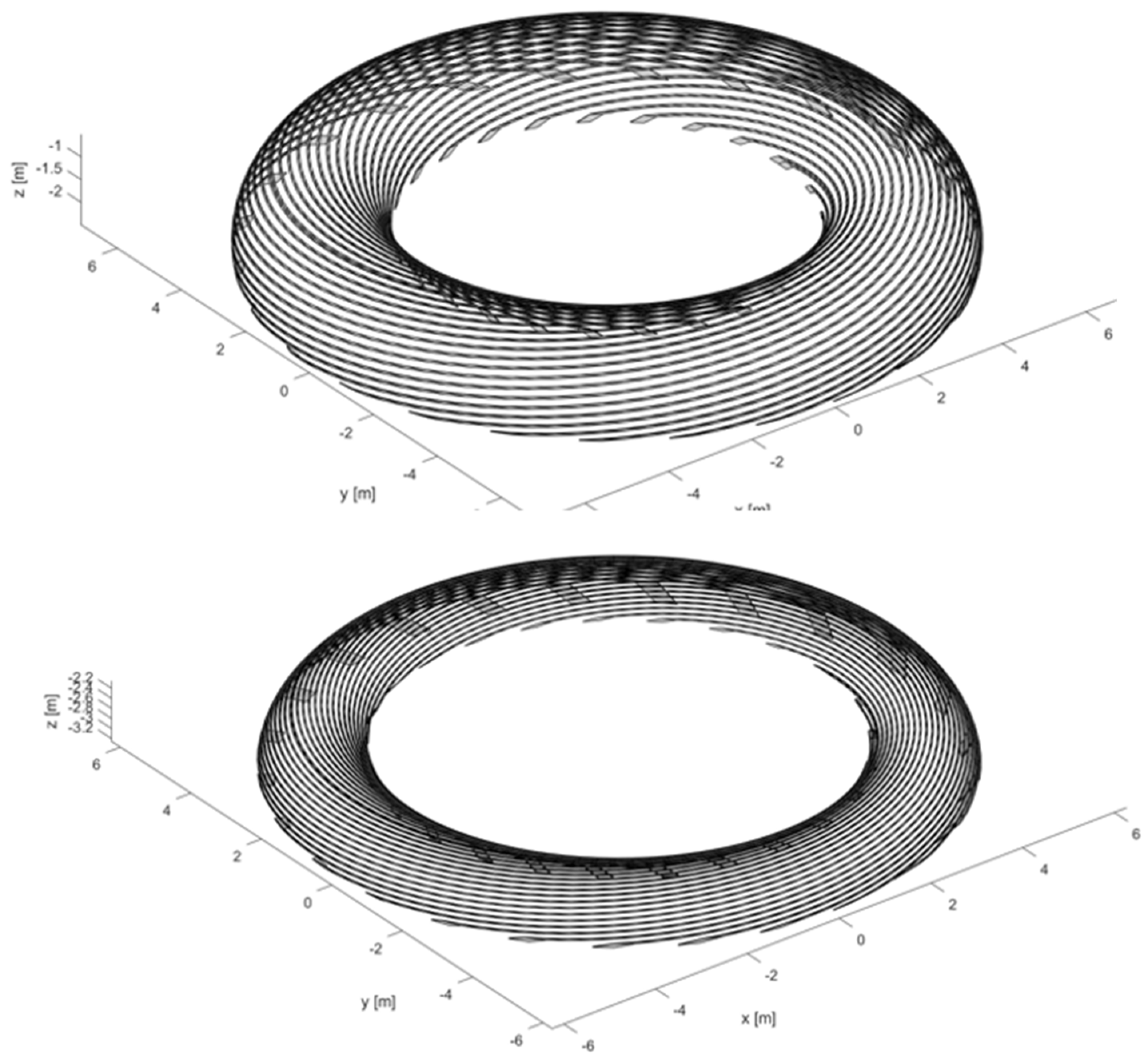
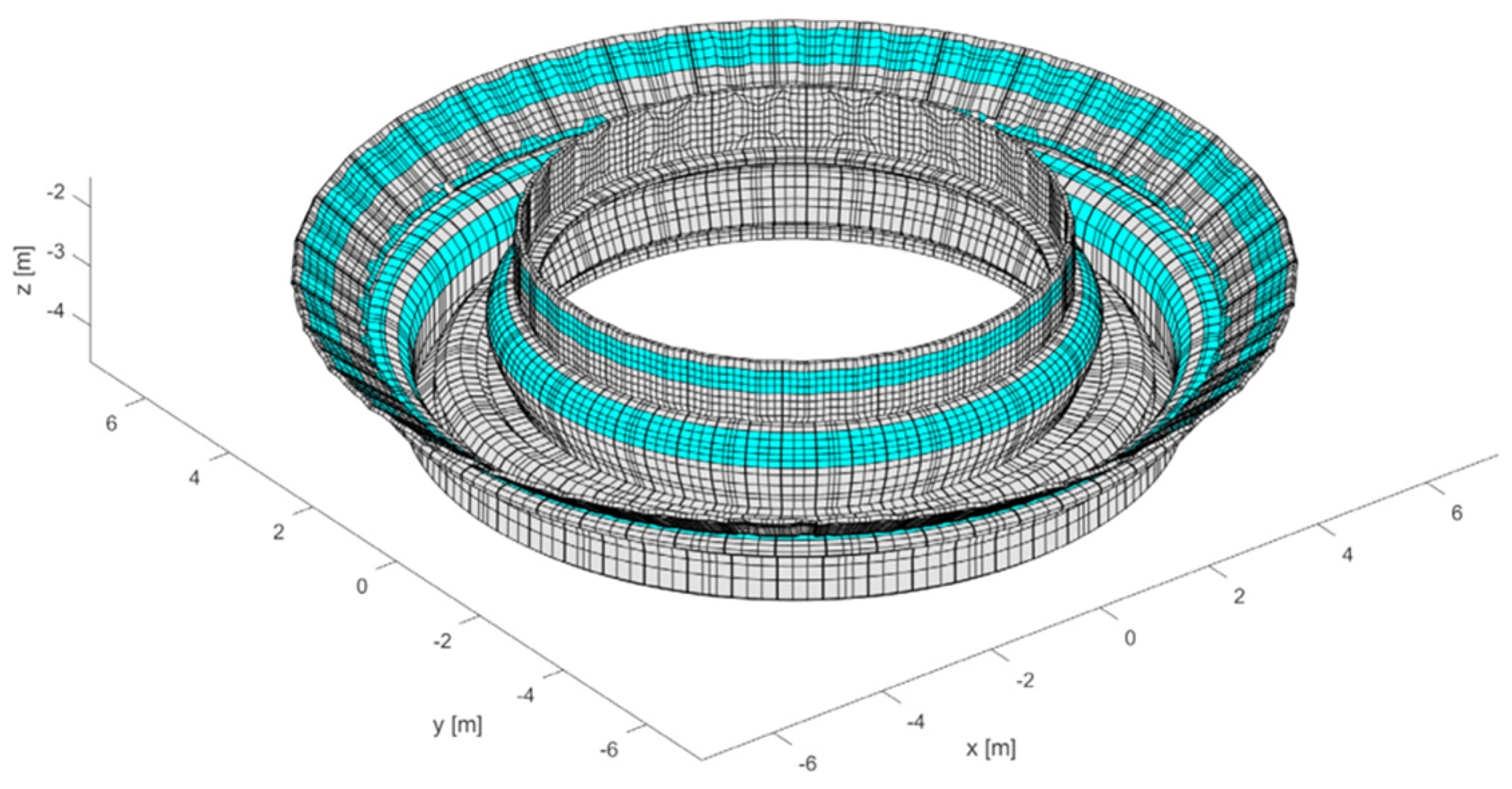
18], the present model simulates gradual compression of the halo layer. For this, the model has four layers of poloidal bridges supplemented by four layers of helical bridges (
Figure 9 and
Figure 10). Symmetric poloidal and anti-symmetric helical halo currents are fed in the corresponding 4 + 4 = 8 layers with consistent modulation in the time (as detailed below), which mimics the gradual compression of the “physical” halo layer.
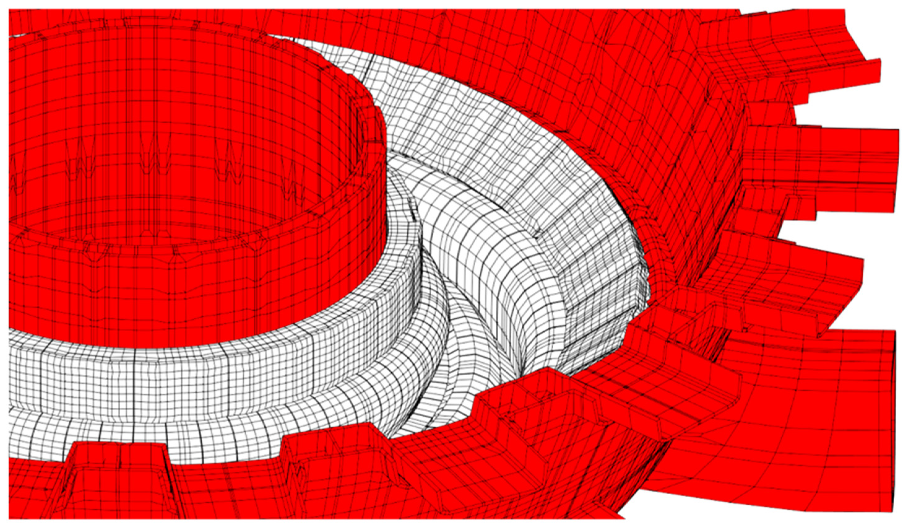
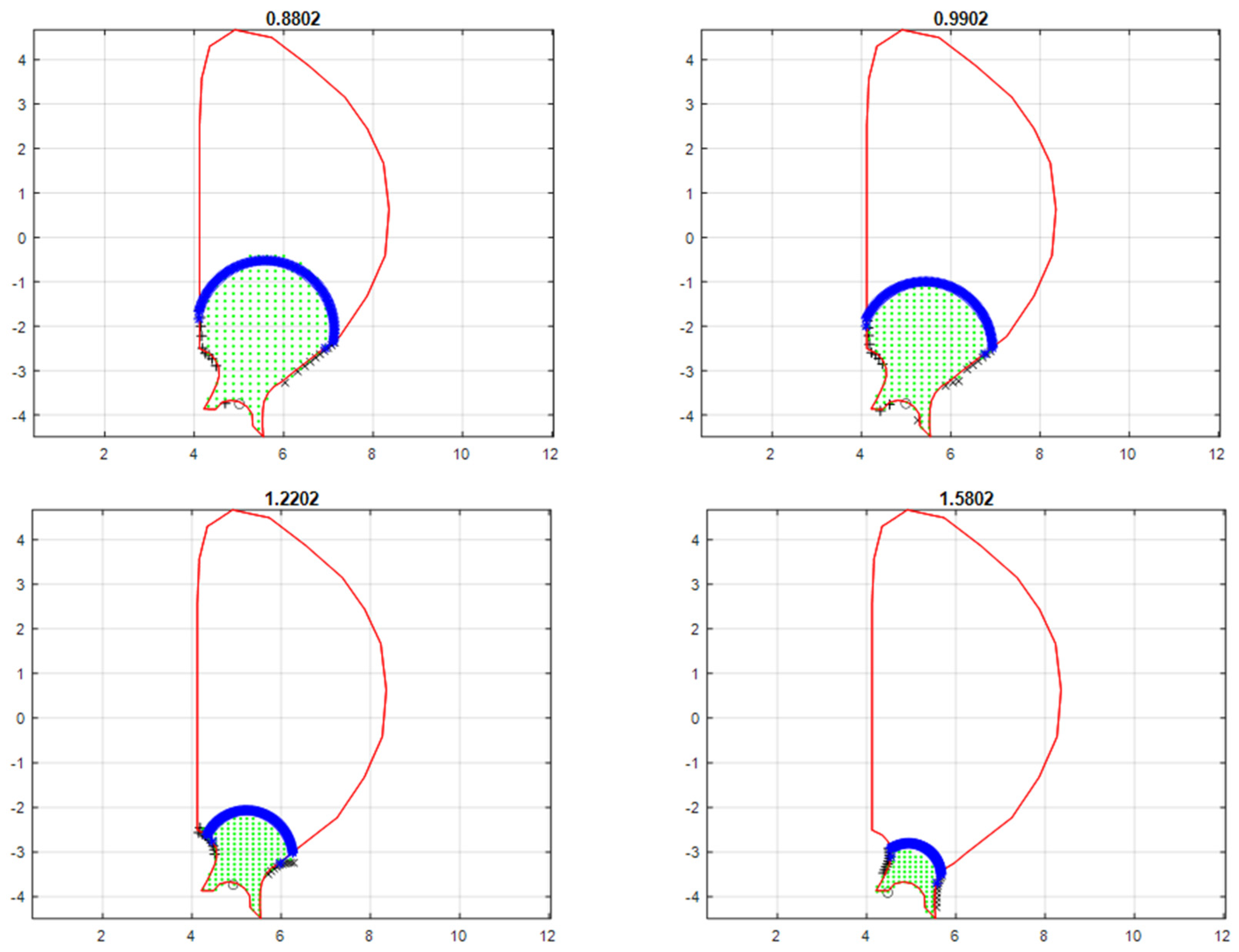
Figure 9 shows the space occupied by four layers of halo bridges wrapping the plasma. Their profiles correspond to the plasma shape at four relevant time instances in the DINA scenario “VDE-Down-Slow-revised”. Each layer encloses (a) 100 poloidal current filaments built for VDE post-processing and (b) 100 helical current filaments added to carry the anti-symmetric halo current components.
Figure 10 illustrates helical filaments of the first and last layer. Each layer intercepts the plasma-facing surfaces on its own pair of toroidal belts, i.e., inboard and outboard (
Figure 11). Four outboard interception belts are well-spaced; however, four inboard belts partially overlap each other and thus look like two belts. This is due to the specific shape of the plasma-facing surfaces.
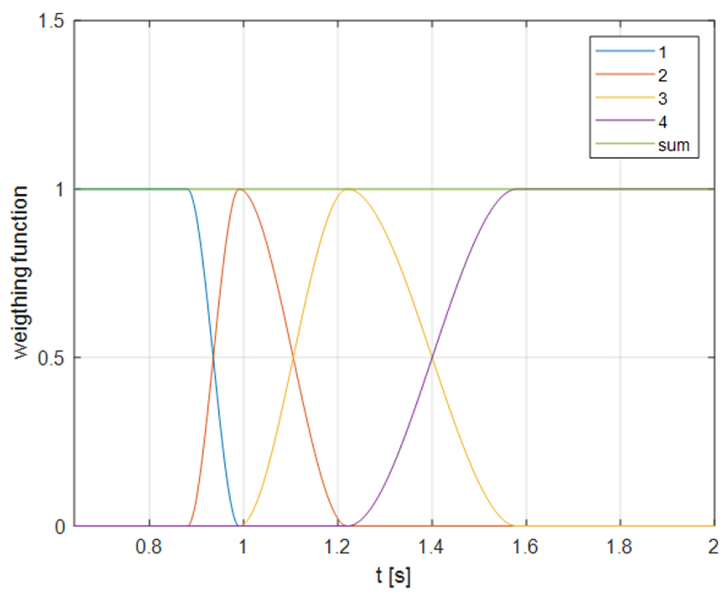
Gradual compression of the halo layer during a VDE and an AVDE is mimicked numerically by a consistent modulation of both poloidal symmetric and helical anti-symmetric halo currents fed in four consequently enclosed layers (
Figure 12). This modulation mimics some in-depth profiles of the halo layer. Presently, the modulation for helical currents is performed in the same way as it was implemented for poloidal currents in the preceding VDE post-processing. This may be refined in further studies for better consistency with the plasma current profile.
The severity of an AVDE is specified here, as an arbitrary input assumption, by the commonly used coefficient TPF (“toroidal peaking factor, peak-to-average ratio”). Note that local current densities defining the TPF are measured normal to a wall, for already superimposed components of poloidal symmetric and helical anti-symmetric halo currents.
In the future, when resources allow, the present EM model with four layers of the halo bridges can be used for a more accurate introduction of gradually growing AVDE distortion. This can be performed with layer-specific time-dependent TPF coefficients TPF1(t)–TPF4(t), growing in time differently one from another to better mimic possible AVDE evolution scenarios. The same model can be used later for the calculation of EM loads from the rotating AVDE, as explained in the next section.
To summarize, features taken from the trial models [
18] are (a) each layer contains 50 pairs of helical filaments and (b) within each pair, two filaments have identical shapes spaced by 180 degrees and carrying an equal modulus but inverted current waveforms.
To explain how the model intrinsically ensures the global balance of EM loads and magnetic fluxes, we use here the term “helix” for each elementary current loop formed by one helical filament and closed through tokamak conductive structures. In each pair of helixes spaced mutually by 180 degrees:
One helix creates three net forces and three net torques by interacting with eddy currents in the VV and with all currents flowing in the windings of the Magnets.
Its “antipode” also creates three net forces and three net torques acting on the VV and the Magnets, with the same six moduli: some co-directional with, but others opposite to, the loads created by the first helix.
The shapes of, and currents in, all paired helixes are such that the superposition of these currents with all plasma currents involved in the preceding VDE post-processing creates a pattern resembling one in the plasma distorted in the kink mode. Of course, such mimicking is not perfect, but to some degree realistic, and suitable for our practical purposes.
The superposition of current waveforms prescribed to all filaments in the plasma volume (toroidal, poloidal, and helical as described), all eddy currents, and currents in the coil windings allows for calculating maps of EM force densities and conclude with waveforms for six net load vectors without duplication or omission, as detailed below.
Regarding the vertical vectors of net loads, each helix creates some vertical net forces and moments acting on the VV and the Magnets. Its “antipode”, having the same shape but opposite current, creates exactly opposite vertical net forces and moments acting on the VV and the Magnets. This means each pair of helixes creates zero net vertical force and moment acting on the VV and the Magnets, and therefore does not disturb the vertical load balance as it was delivered by the preceding VDE plasma evolution simulation code and preserved then at the consequent VDE post-processing.
Regarding the lateral vectors of net loads, due to the 180-degree toroidal spacing between the two paired helixes, combined with their perfectly “mirrored” currents, vectors of lateral forces acting on the VV and the Magnets are not compensated but summed. Similarly for the lateral moments, the 180-degree spacing of the paired helixes results in opposite vertical EM forces acting on the VV and the Magnets on well-spaced parallel lines, thus not compensating but summing. This ends up in serious lateral net forces and moments.
Basically, the above means that the symmetric halo current component contributes only to vertical net forces and moments (two out of six net load vectors), whereas the anti-symmetric pattern contributes exclusively to the lateral net loads (the remaining 2 + 2 = 4 net load vectors). All this is proven by the numerical results presented in the next section.
This EM model could be used, without modification, for the calculation of EM loads during the rotating AVDE, such as described, e.g., in [
15,
20]. The AVDE rotation can be simulated in this model by additional harmonic (in time) modulation of currents in all helical filaments in each layer. However, this article is limited only to the results for the locked AVDE since the calculations of EM loads at the rotating case will require a much longer computing time. Thus, these activities will be the topic of future study.
5. Additional Numerical Procedures Refining EM Load Balance
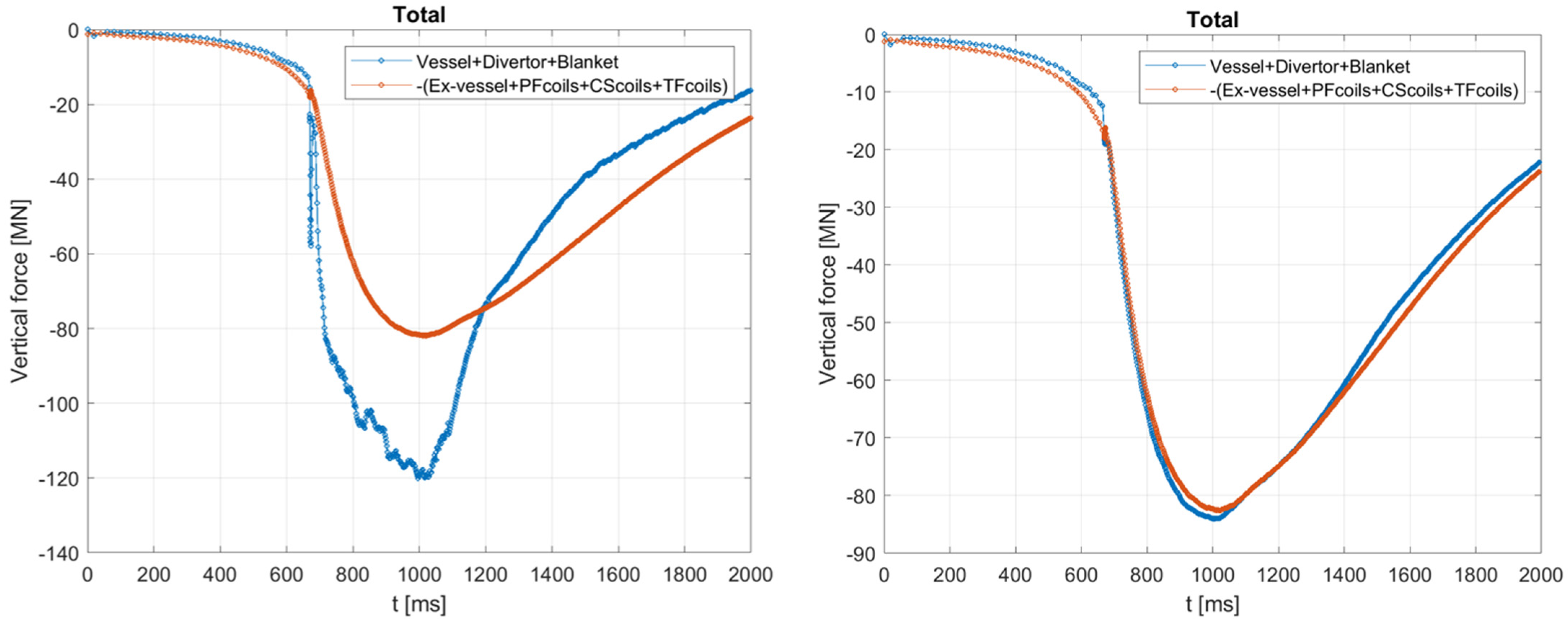
The practical calculations reported here begin from the refined post-processing of the symmetric EM event, the VDE. The goal is to refine the vertical force balance that gets disturbed by numerical reasons. This step is found to be necessary because the DINA VDE scenario used here has not been fine-tuned for the vertical net force balance and because the DINA code employs a simple 2D VV model, whereas EM post-processing codes calculate EM loads on much more detailed 3D EM models. We have refined the vertical force balance by iterative adjustment of the helicity of the (still symmetric) halo current. Specifically, we iterated the waveform of the net poloidal halo current originally prescribed by DINA to meet the criterion of net vertical EM force balance for the entire tokamak. All other parameters of the DINA VDE scenario are kept intact.
Figure 13 shows the vertical net force balance during the VDE (not the AVDE yet), before and after such balancing.
With the previous step completed (balancing of the vertical net forces at VDE post-processing), we begin the calculation of the lateral EM loads for AVDE: transient EM simulations on the 360-degree EM model with four pre-existing layers for the poloidal halo currents and four layers added for the anti-symmetric helical halo currents (
Figure 10). The anti-symmetric helical currents fed in four layers of helical bridges gradually migrate from the outer to the inner layers exactly as it was performed for the poloidal halo currents at VDE post-processing (
Figure 12). The normalized harmonic toroidal distribution of the currents between 100 helical filaments in each layer remains intact and corresponds to
TPF = 1.5.
The three last calculation steps towards the delivery of AVDE-induced EM loads are (a) superposition with results of VDE post-processing, (b) calculation of the time-dependent EM force densities produced by all currents on all modeled parts, and (c) summation of the EM force densities into net load vectors within each group of tokamak systems, the VV and the Magnets, to deliver six graphs for orthogonal vectors of net EM loads.
In the physical world, any tokamak is, of course, a practically closed EM system Equation (1); however, the calculation of EM loads on complex 3D models is never perfect and always accumulates some numerical errors. Such numerical errors are usually in a scale of a few percent for the dominant load vectors but become more significant when referring to the non-dominant load vectors, such as AVDE-induced lateral EM forces in comparison with vertical ones. This is because, in the numerical sense, the non-dominant net loads result from relatively small differences in large opposite force vectors with a similar modulus. This amplifies the accumulation of numerical errors. Since the presented EM loads serve as inputs for simulation of the tokamak’s structural dynamic response to AVDE, we will be as accurate as possible: we will somehow compensate numerically the accumulated EM load imbalances prior to the structural dynamic simulations. Not to mislead the reader, all plots of AVDE loads in next sections show results after the final numerical balancing described in this section. For the sake of brevity, this article does not compare various possible balancing procedures. We investigated two techniques and selected the following one.
Since the directly calculated EM force maps, due to trivial accumulation of numerical errors, cannot achieve a sufficiently accurate balance of lateral loads between the VV and the Magnets, an additional a posteriori correction is provided by superposition of the raw results with the following two suitable force density fields: a toroidal (
) and a vertical one (
). These depend linearly on the horizontal coordinates (
x,
y), as shown in Equation (2), and are added to a portion of the domain, called here “the scaled domain”. It is composed of the VV with internals but without ports. By imposing equilibrium of the integrals of the force densities on the scaled domain with the “target” domain (in this case, the Magnets), as performed in Equation (3) for the forces, six equilibrium equations arise (three net forces and three net moments), and it is possible to solve for the six unknowns (the two slopes and the constant term of each field,
). This is computed at each time step to finally achieve the condition of zero net EM loads (six vectors) for the entire tokamak. The densities of the added force fields found with this approach are on the scale of one or two percent of the raw volume-average modulus of EM force densities calculated directly. This is consistent with typical numerical errors in calculation of EM loads in complex 3D systems and indicates that such final numerical balancing procedures cannot seriously disturb the peak values of dominant EM loads acting on tokamak systems.
6. Practical Results on AVDE-Induced Lateral EM Loads
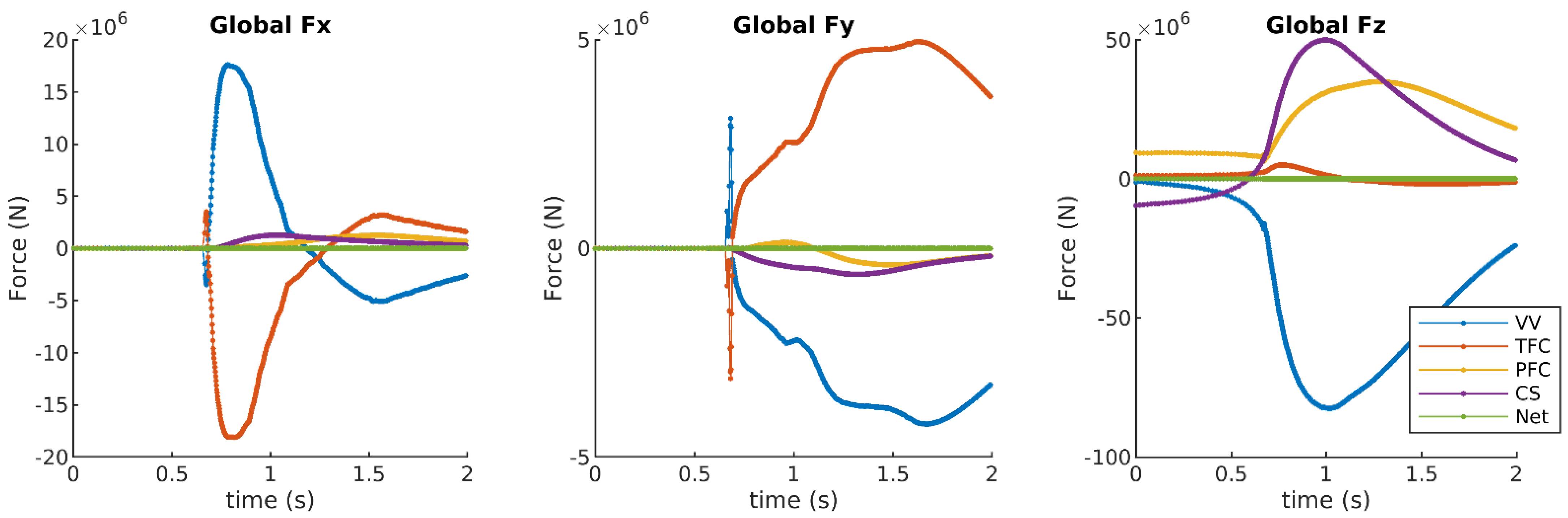
Figure 14 and
Figure 15 show the main practical results including graphs of six orthogonal vectors of AVDE loads applied to the VV with internal components and separately to the CS, PF, and TF coils composed of the windings and cold structures. All six net load vectors for the entire tokamak are close to zero (green lines in
Figure 14 and
Figure 15). These and all other plots in this article correspond to
TPF = 1.5 and incorporate the final numerical balancing described above.
Short spikes on the net force graphs (
Figure 14) correspond to the thermal quench. We consider these spikes of net EM loads as non-physical: they result from an imperfect numerical simulation of the VV EM shielding effect on the 360-degree tokamak model. Such spikes are commonly seen even at VDE post-processing on 40-degree EM models. They are hard to suppress right in the simulations of EM transients because more precise numerical simulation needs to operate with much more heavy FE models with multi-layer representation of VV shells, exceeding computing limits. Some EM post-processing teams recommended removing or reducing such short-lasting peaks at the load transfer on mechanical models of the VV and the Magnets. However, fast EM transients caused by TQ are to be kept for calculation of EM loads at the in-vessel components.
Table 1 collects the extremes for all six vector components of net EM loads for the VV and the Magnets: the plain values show extremes calculated for
TPF = 1.5, whereas the values in brackets offer the linear scaling for a worse AVDE, at
TPF = 2.0. Note that the vertical net loads, Fz and Mz, were obtained numerically the same as they were for the VDE, and not to be scaled with
TPF either. This was highlighted analytically in [
6] and explained in previous sections hereon. Our numerical model keeps such equity as an intrinsic feature.
Table 1 shows the peak lateral net force by a factor of ~2 higher than reported in [
18]. This is due to a combination of model features that have not been combined in the trials.
An AVDE creates quite serious lateral EM moments. Being relatively modest at a VDE, they become a dominant load component at an AVDE and should always be reported in EM studies and included in inputs for consequent mechanical, dynamic, and structural analyses.
It is worth noting that the middle lines in
Table 1 show EM moments calculated at the origin in the tokamak center (located in the horizontal symmetry plane of the TF coils). It is elevated by ~7.5 m over the tokamak supports. This means that lateral net forces shown in the upper lines create additional moments at the level of tokamak supports with arms ~7.5 m. The lateral moments re-calculated to the origin shifted down to the level of the tokamak supports are not plotted; however, they are indicated in the last lines of
Table 1.
From
Figure 14 and
Figure 15 and
Table 1, we can see that, at AVDE with
m = 1,
n = 1, and
TPF = 1.5, the net lateral EM forces at either the VV or the Magnets reach ~20% of the peak vertical forces; however, AVDE-induced lateral moments at either the VV or the Magnets exceed the peak vertical moments by a factor of 35.5, thus becoming quite important load components.
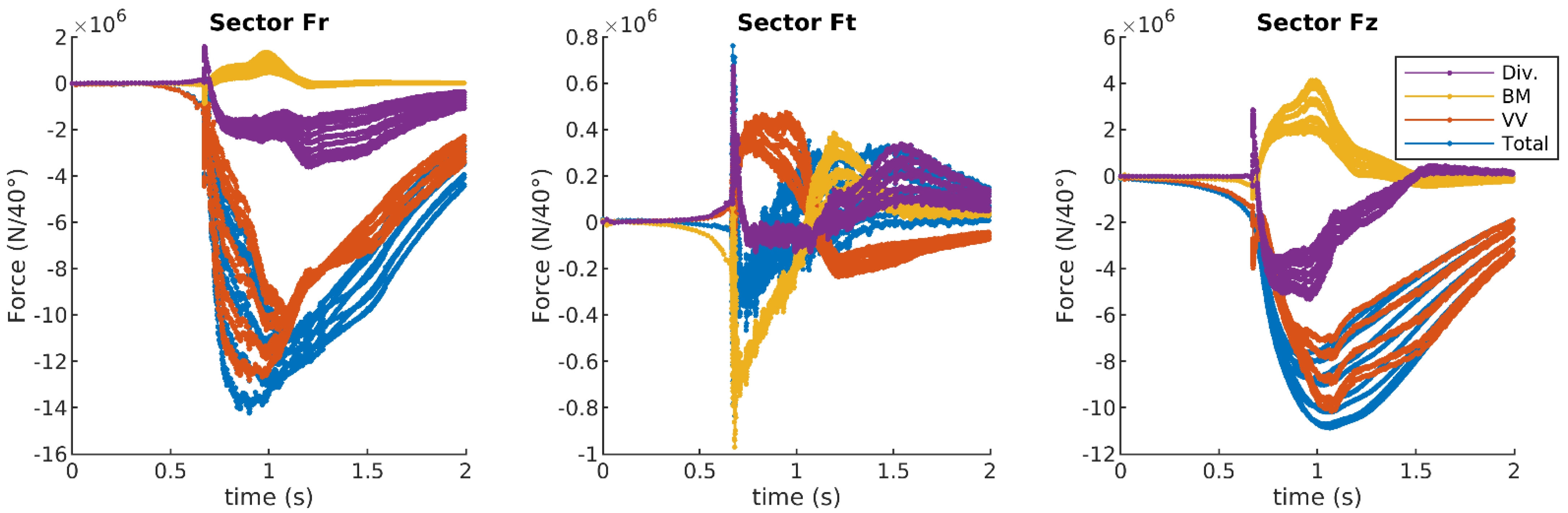
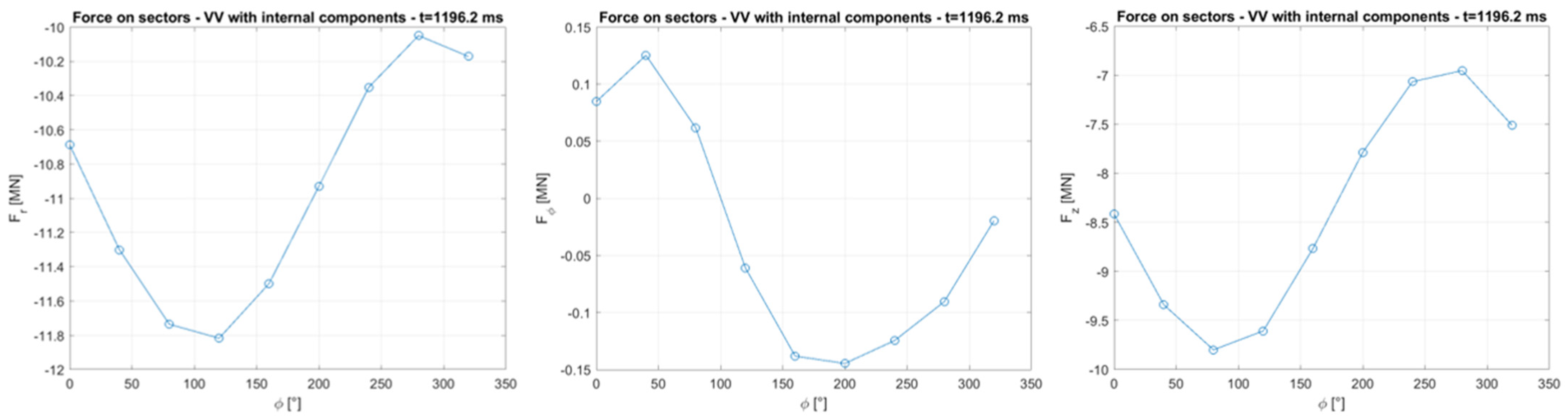
Figure 16 shows, in cylindrical coordinates, graphs of three vectors of AVDE-induced net EM forces for each of the nine 40-degree sectors of the VV with internal components, with sub-divisions for forces on the blanket, divertor, and the VV itself (composed of the VV shells, ribs, and ports and ports extensions). We can see that the graphs for the toroidal force are noisier than the rest of the computed forces: this is because this force vector is an order of magnitude smaller than the others and thus more sensitive to the residual numerical noise.
Figure 17 illustrates the toroidal variation in three orthogonal net forces for the nine VV sectors with relevant internal components at the specific time instant t = 1.1962 s.
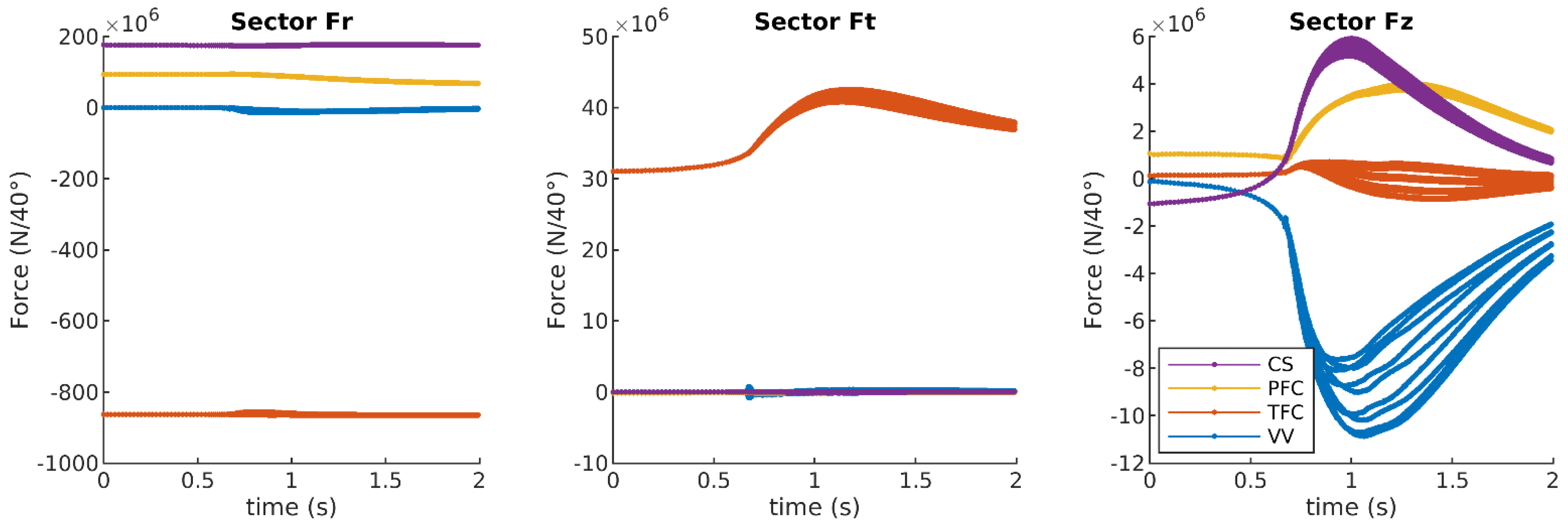
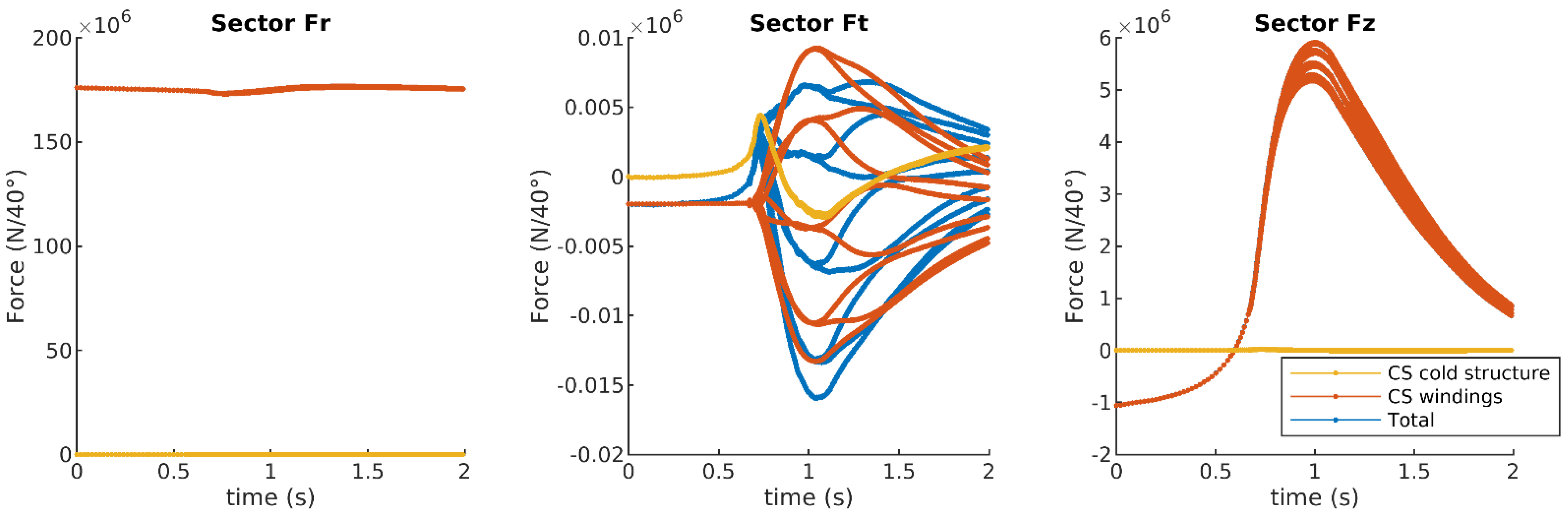
Figure 18 combines, in cylindrical coordinates, graphs of local radial, toroidal, and vertical AVDE-induced EM forces found separately for each of the nine 40-degree sectors of the CS, PF, and TF coils with relevant cold structures and forces found for each of the nine 40-degree sectors of the VV with relevant internal components.
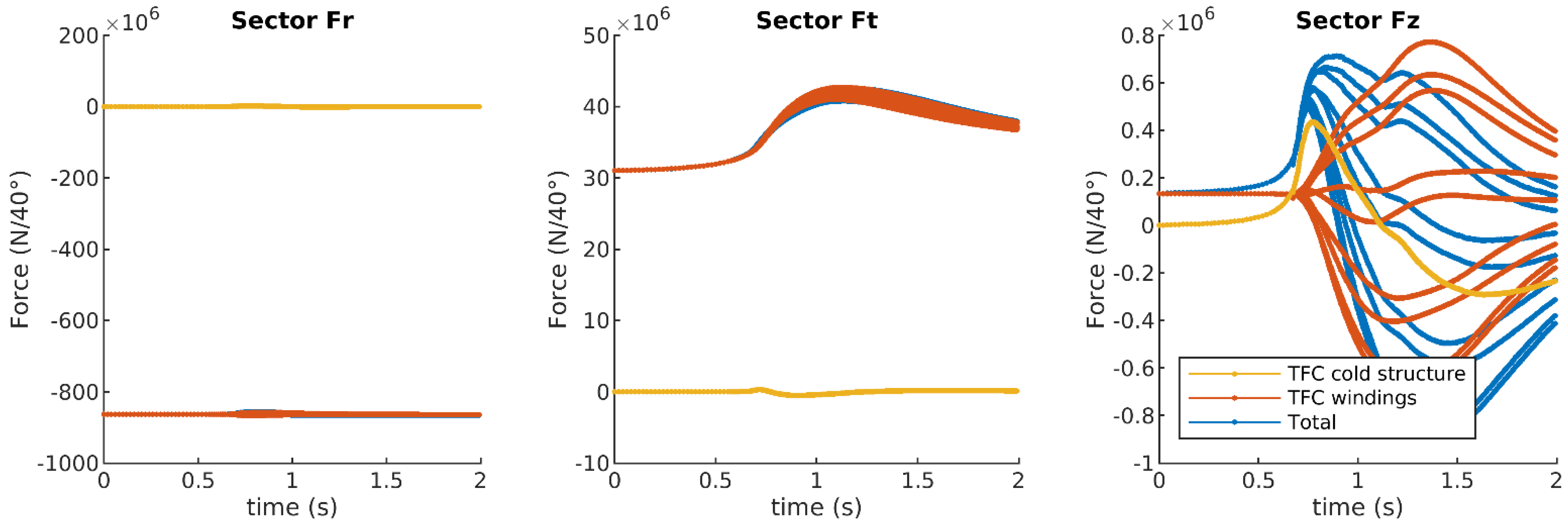
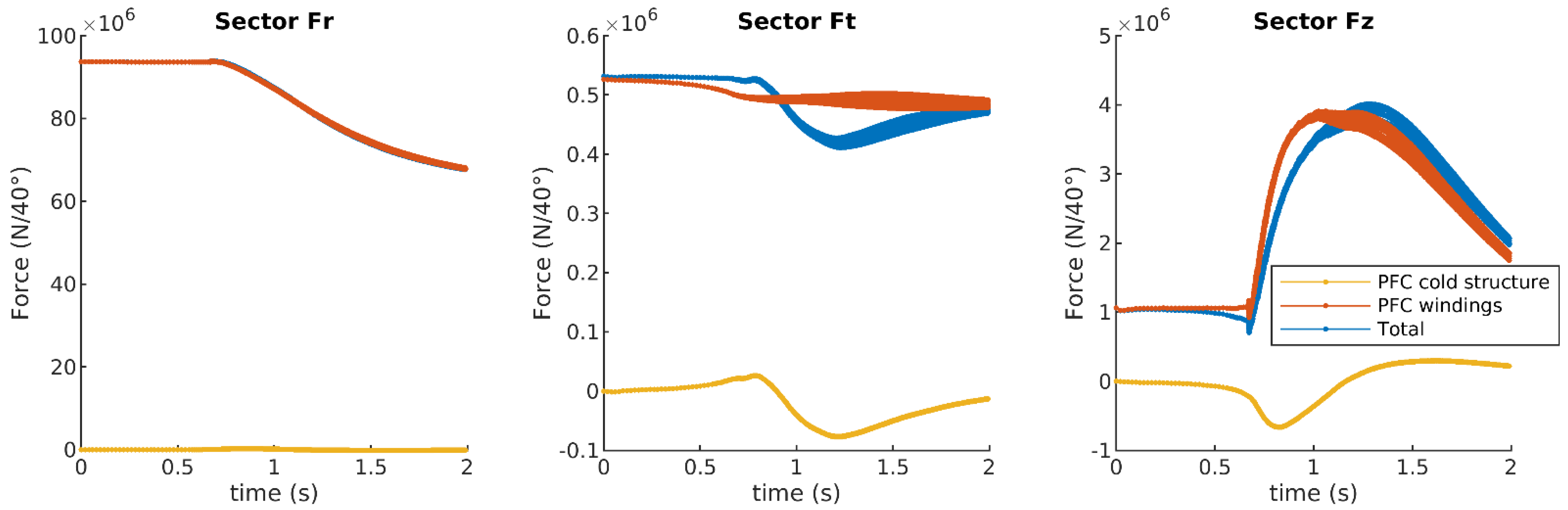
Figure 19,
Figure 20 and
Figure 21 show, in cylindrical coordinates, graphs of local radial, toroidal, and vertical EM forces for each of the nine 40-degree sectors of TF, PF, and CS coils with relevant cold structures.
In terms of the
vertical net forces, the EM interaction remains similar to that at the VDE:
Figure 14,
Figure 16,
Figure 18,
Figure 19,
Figure 20 and
Figure 21 show that net vertical forces acting on the VV are compensated mostly by vertical reaction forces on the CS and PF coils. However, net lateral AVDE-induced forces on the VV are compensated mostly by net lateral reaction forces on the TF coils.
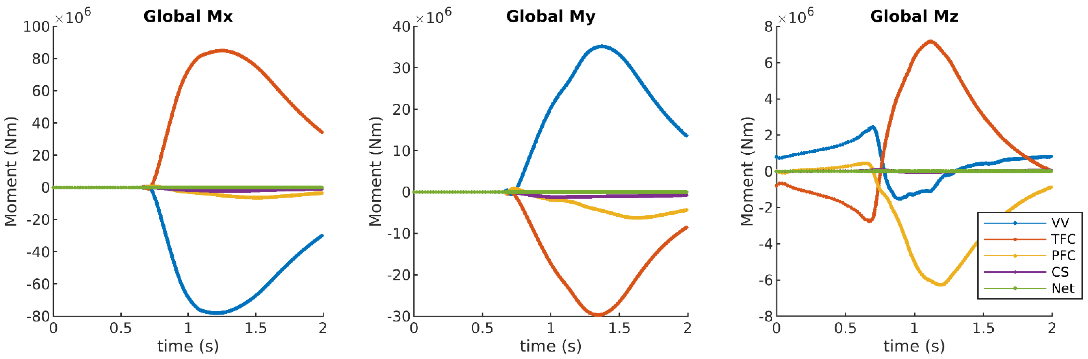
Figure 15 shows the compensation of the
lateral net moments (
Mx and
My): AVDE-induced lateral moments acting on the VV (a) seriously exceed the vertical moment and (b) are compensated mostly by opposite lateral moments acting on the system of TF coils.
There are quite different ratios of the lateral to the vertical net load vectors: with the input assumption of TPF = 1.5, peak lateral forces are limited by one-fifth of the peak vertical forces, while peak lateral moments greatly exceed the vertical ones (by a factor of 35.5 for Mx). One may refer to a rather small denominator, but anyway, AVDE-induced lateral moments are large on their own. As a practical conclusion, any results for AVDE-induced EM loads should always be reported including the net lateral moments, not only the lateral forces.
The reported results show that both at the VDE and AVDE, not large but noticeable vertical moments (
Figure 15) are produced by the EM interaction between the VV and the Magnets. These moments have been noticed earlier by several EM analysis teams, still in the conditions of VDE. However, to our knowledge, these explanations are not worded in papers. We can explain non-zero vertical moments between the VV and the Magnets (
Figure 15) by the interaction of three cyclic (both at the VDE and AVDE) current patterns as follows: (a) poloidal currents in 18 discrete TF coil windings, (b) helical VV eddy currents deviating around VV ports and (c) “saddle” eddy currents looping within a case of each TF coil and in nine electrical sectors of cold structures assigned to the CS and PF coils. In the ITER, the VV and almost all cold structures have 9-fold toroidal cyclic symmetry. However, the TF coils cause field ripple with 18-fold cyclic symmetry. We think that the interaction of all three cyclically distorted current patterns, having some mutual toroidal phase shifts, is responsible for the reported non-zero vertical moments between the VV and the Magnets. This slightly resembles EM interaction in AC motors. Such interaction of cyclic current patterns involves even arc-shaped sectors of PF coils. All the above-listed contributors are highly design-dependent, making the net vertical moments also design-dependent, but, in any case, mutually compensated by the conservation law.
The plots for lateral forces in
Figure 14 show that the force vector along the X-coordinate
Fx = +17 MN reaches its maximum at t = 0.8 s; however, the force vector along the Y-coordinate
Fy = −4.1 MN peaks at 1.7 s. This means the following. If experimental observations of AVDE evolution are based on mechanical measurements for vectors of lateral VV forces, then even the permanently locked AVDE can easily make an impression that the AVDE distortion rotates by just 90 degrees and then locks for some reason. However, the numerical results presented here show it as a pure EM effect of the permanently locked AVDE.
It is worth noting that, in many tokamaks, the supports of the VV and the Magnets, and numerous inter-coil links are optimized to react mostly to vertical forces and allow for sufficient freedom for cyclic thermally (or EM) induced radial displacements. For these reasons, relatively modest toroidal reaction forces applied to individual supports of the VV, the magnet supports, and inter-coil links can play quite a significant structural role and accordingly should be quantified as accurately as possible.
7. Further Work
Further work steps can include the following. They will be attempted sooner or later as resources allow.
Select and employ advanced input assumptions on AVDEs evolving with a gradual transition from a VDE to an AVDE by assuming a TPF not constant but gradually growing in time, and perhaps layer-specific. This can be performed on the presented EM model.
Calculate EM loads for the rotating AVDE on the presented EM model, by applying gradually growing (in time) phase shifts in the harmonic toroidal modulation of the halo currents in the filaments forming the helical bridges.
Keeping in mind that this article presents results for the Downward AVDE, provide similar EM calculations for the Upward AVDE, and combine these with a change from the constant to the gradually growing TPF, and with AVDE rotation. This will require partial modification of the EM model (re-building of all halo bridges).
Develop an advanced procedure for the summing of elementary EM force densities on complex 3D numerical models with the purpose of minimizing the accumulation of numerical errors in the composition of large opposite elementary force vectors, to relax the need for the final load balancing by numerical means.
Investigate AVDE scenarios with gradually evolving helicity of the halo layer, by the re-building of all or some of the enclosed layers of helical filaments.
Select the most suitable parameter ranges and preferred combinations of inputs for calculation of the AVDE loads based on matched physics simulations using, for example, M3D-C, NIMROD, JOREK [
7], or other modern specialized non-linear MHD plasma evolution codes.
8. Discussion and Conclusions
This article offers the first practical contribution to a parametric library of ready-to-use time-dependent maps of EM force densities and waveforms of net AVDE-induced loads (orthogonal forces and moments) at the VV and the Magnets. Once the library is at least partly implemented, several variants of time-dependent maps of EM force densities in main tokamak systems will be readily available for their transfer to mechanical dynamic models for the simulation of the tokamak dynamic response to AVDEs. The first set of AVDE loads has been computed with the input on AVDE evolution derived from the scenario “VDE Down Slow revised” taken from the ITER’s DINA library. The present results assume, as the input, a constant in time TPF = 1.5. They can be scaled up or down with TPF variation. Other variants of the parametric results, such as the rotating AVDE and AVDE evolving from “VDE Upward Fast”, may be produced using the same approach. The main parametric variables for further work can be set up as graphs of the following:
Graph of the layer-specific TPF coefficients growing in time will be used to calculate AVDE loads assuming a smooth transition from VDE to AVDE. This can be performed with the present FE model.
A steadily growing in time phase shift can be applied to the harmonic toroidal modulation of currents fed in all helical filaments to calculate EM loads for the rotating AVDE. This can also be performed with the present EM model.
Gradually changing AVDE helicity can be introduced by different helicities of the enclosed bridges. This will require re-building the helical bridges in the model.
The ratio of lateral to vertical AVDE-induced EM
forces is found as ~20% at
TPF = 1.5 or ~40% at
TPF = 2.0 (17 MN/85 MN and 34 MN/85 MN). These peak forces still fit in the limit 48 MN and ratio < 56% (48 MN/85 MN) known for the ITER (e.g., [
16]).
The modulus of the maximal lateral moment Mx exceeds the peak vertical moment by a factor of 35.5 at TPF = 1.5 and accordingly by a factor of 71 at TPF = 2.0 (78 MN×m/2.2 MN×m and 156 MN×m/2.2 MN×m). This is partly because of a quite modest denominator, but AVDE-induced lateral moments are serious on their own: My = 135 MN×m at TPF = 1.5 and My = 270 MN×m at TPF = 2 (both with the origin at the level of tokamak supports). We cannot compare the reported herein lateral moments with ones in other AVDE studies since we are not aware of reports on AVDE-induced lateral moments for ITER-scale tokamaks. Accordingly, it is worth highlighting that any AVDE studies, with any AVDE model, should report not only lateral EM forces but also lateral EM moments at the VV and at the Magnets.
It is important to remember that all results shown here are not intended for direct use for the purposes of load specification but just to fill the first cell in the library of AVDE loads. Other cells are to be filled with parametrically varied input assumptions on AVDE form and severity. The physics community may either recommend specific sets of inputs (in the terms explained hereon) or suggest the ranking for variants found in the AVDE loads library. This will help to choose variants of ready-to-use AVDE loads suitable as input for in-depth engineering analysis, such as mechanical dynamic simulations followed by the structural sub-modeling. At today’s initial stage, the reported AVDE loads can fill not a cell but a row in the AVDE library since they can be scaled up and down with TPF.

 ,
, 


