Article

A Boltzmann Electron Drift Diffusion Model for Atmospheric Pressure Non-Thermal Plasma Simulations

Department of Electrical, Electronic and Information Engineering, University of Bologna, 40136 Bologna, Italy
*
Author to whom correspondence should be addressed.
Plasma 2023, 6(3), 393-407; https://doi.org/10.3390/plasma6030027
Submission received: 28 April 2023 / Revised: 4 July 2023 / Accepted: 5 July 2023 / Published: 7 July 2023
(This article belongs to the Special Issue Dielectric Barrier Discharges 2023)

Abstract

:
We introduce a fluid computational model for the numerical simulation of atmospheric pressure dielectric barrier discharge plasmas. Ion and neutral species are treated with an explicit drift diffusion approach. The Boltzmann relation is used to compute the spatial distribution of electrons as a function of the electrostatic potential and the ionic charge density. This technique, widely used to speed up particle and fluid models for low-pressure conditions, poses several numerical challenges for high-pressure conditions and large electric field values typical of applications involving atmospheric-pressure plasmas. We develop a robust algorithm to solve the non-linear electrostatic Poisson problem arising from the Boltzmann electron approach under AC electric fields based on a charge-conserving iterative computation of the reference electric potential and electron density. We simulate a volumetric reactor in dry air, comparing the results yielded by the proposed method with those obtained when the drift diffusion approach is used for all charged species, including electrons. We show that the proposed methodology retains most of the physical information provided by the reference modeling approach while granting a substantial advantage in terms of computation time.

1. Introduction

Dielectric barrier discharges (DBDs) are well known as being one of the most efficient ways to generate a non-thermal plasma in atmospheric pressure air [1]. Originally developed for the generation of ozone [2]. DBD-based apparatuses are now used in a wide spectrum of scientific, industrial, and biomedical applications. The DBD shares many characteristics with the corona discharge, although the latter term is preferred for discharges between bare metal electrodes without solid dielectrics [3]. Due to the presence of one or more dielectric barriers between the electrodes and the gap, the design of DBD reactors can be optimized to achieve the discharge uniformity properties required for industrial surface treatments [4]. Surface DBD configurations have also been extensively studied and applied in the aerospace field, mainly for flow control related applications [5,6,7]. In the life sciences field, DBDs are currently studied for the abatement of volatile organic compounds [8] and the inactivation of airborne [9] and foodborne [10] viruses. Other applications in this field include wastewater treatment [11,12] as well as disinfection/sterilization of food [13] and surfaces and medical devices [14] contaminated by microorganisms.
The above list of applications, far from exhaustive, provides an idea of how broad applications of DBDs are. Bound to this versatility is the need to understand and ultimately control the operation of these devices, as well as the mechanisms behind the generation and quenching of the many chemical species produced in different gases and physical conditions [15]. In this sense, computational models of these devices represent an important source of knowledge, more so due to the complexity and cost of spectroscopic measurements that are typically needed to perform investigations on discharge properties [16]. In addition, computational models for assessing large electric fields in the presence of mobile charge carriers may also be useful in other fields, such as the design of accelerating fields in laser-plasma acceleration applications [17].
Historically, the vast majority of computational models for high-pressure non-equilibrium discharges are based on a fluid description, where each considered species is described by means of a number density and a momentum transfer conservation equation, integrated over time [18,19]. Differently from the case of other non-equilibrium discharge types, e.g., the ones in plasma thrusters, quasi-neutrality conditions cannot be assumed for DBDs. Hence, the space-charge electric field must be calculated self-consistently with the charged particle transport and generation rate [20]. This is commonly performed by coupling the fluid conservation equations to Poisson’s equation for electrostatics.
Recently, Shaygani and Adamiak proposed a simplified algorithm to study a plasma flow control actuator [7,21]. They implemented a three-species fluid model in COMSOL Multiphysics and limited discharge pulses by adding a dumping term to the electron charge transport equation in order to decrease the simulation time. They conducted the simulations in COMSOL using the implicit backward differentiation formula for integrating over time. Sato et al. also presented a method to speed up simulations of surface DBDs [22]. Under the assumption of small space-charge modification, they calculated the time–electric field variations instead of directly solving the Poisson equation at every time step. They evaluated the fluxes with the Scharfetter–Gummel scheme and performed the time integration using the first-order Euler implicit method. Nakai et al. investigated the influence of chemical reactions on the EHD force generated by a DBD plasma actuator [23] using a three-species finite-volume approach. Regarding the drift term, an upwind scheme with MUSCL interpolation was used, and time integration was performed with a second-order explicit Runge–Kutta method. Hua and Fukagata examined the evolution of nanosecond-pulsed DBD with different electrode polarities [24]. They used the Sharfetter-Gummel scheme for the spatial discretization and performed an explicit integration over time. The same spatial scheme was used in conjunction with an implicit Euler time integration for the ionic wind model proposed by Sato et al. [25]. Emmons and Weeks proposed a 0-D steady-state model using a limited set of species and reactions [26]. Their simplified model showed close agreement with previous time-dependent simulations. Finally, recent works by Zhong et al. [27] and Zhang et al. [28] have shown promising results in using deep neural networks to speed up simulations of atmospheric pressure discharges of this kind.
As one can see from the above list of modeling works, improving the computation time is still one of the main driving forces for scientific development in this field. As anticipated, the de facto standard for atmospheric pressure non-thermal plasma models is to describe both electron and ion dynamics with a drift diffusion approach [29,30]. This allows one to easily compute the volume charge density ρ at the given time instant, and to self-consistently formulate the electrostatic problem as a linear Poisson problem. Unfortunately, the large mass ratio m i / m e between ions and electrons causes the dynamics of the two species to be very different from each other. Hence, considering an explicit integration, the employed time step Δ t must be small enough to follow the dynamics of the fastest species, i.e., electrons. To achieve numerical stability, this quantity is restricted by the well-known Courant–Friedrichs–Lewy (CFL) condition:
Δ t < 1 | μ s E / Δ + | 2 D s / Δ 2 | ,
where Δ represents the grid spacing; μ s and D s are the mobility and diffusion coefficients of the given species, respectively. For large values of E, it is not uncommon for the time steps to be well below the picosecond range.
Historically, this strong limitation (in addition to the additional constraint imposed by the dielectric relaxation time [31]) has led to the development of several techniques to increase the allowed time step lengths. During the 1990s, Ventzek et al. [32,33] and Punset et al. [34] introduced semi-implicit approaches, which have also been adapted to parallel architectures in later works, such as the one by Lin et al. [35]. Recently, Teunissen [36] proposed an explicit approach based on limiting numerical fluxes based on dielectric relaxation time. Subsequently, this technique has been used by [37] in a surface DBD model using a curvilinear mesh.
In this work, we propose a numerical technique that allows substantial efficiency improvements in fluid codes based on the drift-diffusion approximation. The main idea that will be described in Section 2 is to use a nonlinear electrostatic formulation, where the Boltzmann relation is used to relate the local electron number density and electric potential. This allows to omit electrons from the drift diffusion equations, and to adopt grid spacing larger than the Debye length, with substantial beneficial effects in terms of computational efficiency [38,39]. Although this approach is well-established for hybrid fluid/particle-in-cell models used for low-pressure applications [40], e.g., for plasma thruster modeling [41,42], the authors of this work are not aware of applications of this technique to atmospheric pressure problems involving high voltages that change over time. Using the Boltzmann relation is not trivial under such conditions, both from the purely numerical point of view (the exponential term can become problematic for large positive arguments) and from the perspective of charge conservation. We develop a robust numerical technique to deal with such numerical challenges arising from applied voltages varying in time in the k V range. Subsequently, in Section 3, we simulate a closed volumetric DBD reactor operating with dry air using both the proposed methodology (that will be referred to as Boltzmann drift diffusion) and a classic approach where all species are treated with the drift diffusion technique. The performed comparison shows that the proposed Boltzmann drift diffusion approach allows one to retain the main physical characteristics of the discharge while granting a substantial improvement in the code execution time.

2. Model Description

We describe here the main features of the proposed fluid model. We treat ions and neutrals differently from electrons. The former heavy species are described by means of a drift diffusion approach, commonly employed in atmospheric pressure plasma models. Therefore, we provide a concise description of the heavy species treatment and focus more on the numerical strategy used to describe the electron transport. We also refer the reader to [15,30] for a description of the explicit methodology used for the time discretization of the equations and to [43] for the semi-implicit technique employed for the source terms’ integration.

2.1. Ions and Neutrals—Drift Diffusion Approach

The number density conservation equation for the generic species s number density is [44]:
n s t + · Γ s = Ω s ,
where Γ s = n s u s represents the flux due to the mean velocity u s of the species s. On the right-hand side (RHS) of (2), Ω s is the source term for s and describes the rate at which particles are created or destroyed due to kinetic processes. The drift diffusion approximation consists of assuming that advection is only due to electric fields, neglecting the contributions of bulk flow. In this way, the flux Γ s is expressed by means of two contributions, one due to the electric field (drift) and the other due to diffusion:
Γ s = ± n s μ s E D s n s .
The quantities μ s and D s in (3) are the given species’ electrical mobility and diffusion coefficients, bound by Einstein’s relation:
D μ = k B T e ,
where e is the elementary charge, k the Boltzmann constant, and T the temperature in K . The method used to obtain the electric field in (3) is described in Section 2.3.

2.2. Finite Volume Discretization

The integration of (2) over a generic control volume (CV) V, bounded by a closed surface V with an outward pointing normal n ^ , yields:
d N s d t = V Γ s · n ^ d S + P s ,
where N s = V n s d V ; the quantity P s = V Ω s d V is the number of particles produced (or eliminated) within in the volume V by the kinetic processes, per unit of time.
A cell-centered finite volume (FV) discrete formulation of the drift diffusion equation can be obtained by applying the integral form of (5) to the generic control volume V i . Assuming a uniform number density over V i , one has N s , i = V i n s d V n s , i V i . Then, extending the reasoning to the source term, we have P s , i = V i Ω s d V Ω s , i V i . The FV discretized expression reads as:
d n s , i d t = 1 V i A p V i Φ A p ( Γ s ) + Ω s , i ,
where Φ A p ( Γ s ) is the integral flux of Γ s over the generic face A p of the CV.
There is vast literature on different numerical strategies for the approximate evaluation of the transport term Φ A p ( Γ s ) in (5); see, e.g., [45,46]. Considering a 1-D case for the sake of simplicity, a second-order accurate approximation of diffusive fluxes is usually obtained through the finite centered difference scheme:
A p D s n s n d S D ¯ s n s , i n s , j Δ i , j A p ,
where Δ i , j is the length associated to the given interface and D ¯ s the average between D i and D j , the diffusion coefficients evaluated at the generic adjacent nodes i and j. The most popular existing techniques for the drift term ± n s μ s E can be (non-exhaustively) grouped into two broad categories. These are schemes yielded by Taylor series approximations of the nodal number density values or obtained via exponential fittings of exact solutions. The first-order upwind scheme (UDS) is the simplest methodology in the first group. Its popularity is mainly due to its robustness and absence of oscillation. This is the methodology used in this work:  
A p n s μ s E n d S n s , i v s , + + n s , j v s , A p ,
where v s , + = max ( 0 , μ s , i E n ) and v s , = min ( 0 , μ s , j E n ) . E n is the electric field component perpendicular to the interface surface A p , while μ s , i and μ s , j are the electrical mobilities evaluated at nodes i and j. Higher-order methods, introduced to mitigate the well-known artificial diffusivity of the UDS scheme [46], are also commonly employed in computational fluid dynamic codes. The increased accuracy of higher-order schemes comes at the cost of losing the numerical stability of the UDS. For a flow characterized by a large Peclet number, i.e., a strongly advection-dominated problem, numerical stability can be (at least partially) recovered using a flux limiter [45].
Regarding the exponential fitting techniques, the Scharfetter–Gummel (SG) scheme [47] allows the drift and diffusion fluxes to be integrated in a single step. The SG scheme, ubiquitous in semiconductor modeling, has also been extensively used by the plasma modeling community both in its original form [29,33] and in improved higher-order implementations [48,49,50]. The reader is referred to the comprehensive work of Nguyen and colleagues for details on the SG scheme [50].

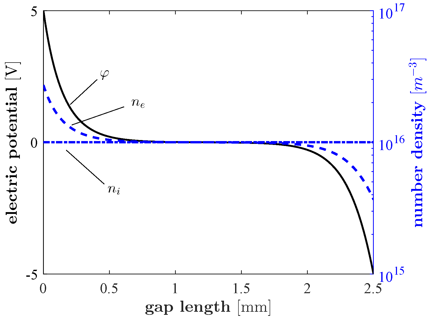
2.3. Electrons—Poisson–Boltzmann Problem

The electric field E appearing in (3) depends on several factors. These are the externally applied voltages, volumetric charge densities resulting from the spatial distribution of the charged species, and surface charge densities accumulated on interfaces. Assuming that the field is conservative, the electric potential φ is given by Poisson’s equation:
· ϵ r φ = ρ ϵ 0 ,
in which ϵ 0 is the vacuum electric permittivity and ϵ r the relative electric permittivity of the considered media. The volumetric charge density ρ at a given time instant is given by the charged species number densities distribution, as in:
ρ = s q s n s ,
where q s is the elementary charge (with sign) associated with the species s. In the standard approach in which the drift diffusion equation (2) is written for all species, the charge density in (10) is evaluated at each time step and used to compute the RHS of (9). Therefore, the Poisson problem is linear with respect to φ .
Alternatively, one may assume that the dynamics of electrons are much faster than those of ions. As a result of this, the electron number density instantly adapts to the local value of the electric potential. This is expressed by the Boltzmann relation:
n e = n e , 0 exp ( φ φ 0 T e ) ,
where T e is the electron temperature in Volt; n e , 0 and φ 0 are reference values for the electron number density and the electric potential. The reader can find a derivation of (11) from the momentum conservation equation in many plasma physics textbooks, such as [51] or [44].
Substituting Equation (11) into Equation (9), a non-linear Poisson problem is obtained:
· ϵ r φ = 1 ϵ 0 s i q s n s e n e , 0 exp ( φ φ 0 T e ) .
The first term in the RHS of Equation (12) represents the charge density due to the ion species. The other term is the charge density due to electrons.
The numerical solution of (12) can be obtained using the well-known Newton–Raphson algorithm. As an example, Figure 1 shows the electric potential distribution and electron number density obtained on a 2.5   m m domain, with a uniform number density of ions ( n i = 1 × 10 16   m 3 ) when Dirichlet boundary conditions ( φ L = 5   V , φ R = 5   V ) are enforced at the two ends of the domain. The term n e , 0 is computed as n e , 0 = Q 0 / ( q e V ) , where Q 0 is the net ion charge and V the discharge volume.

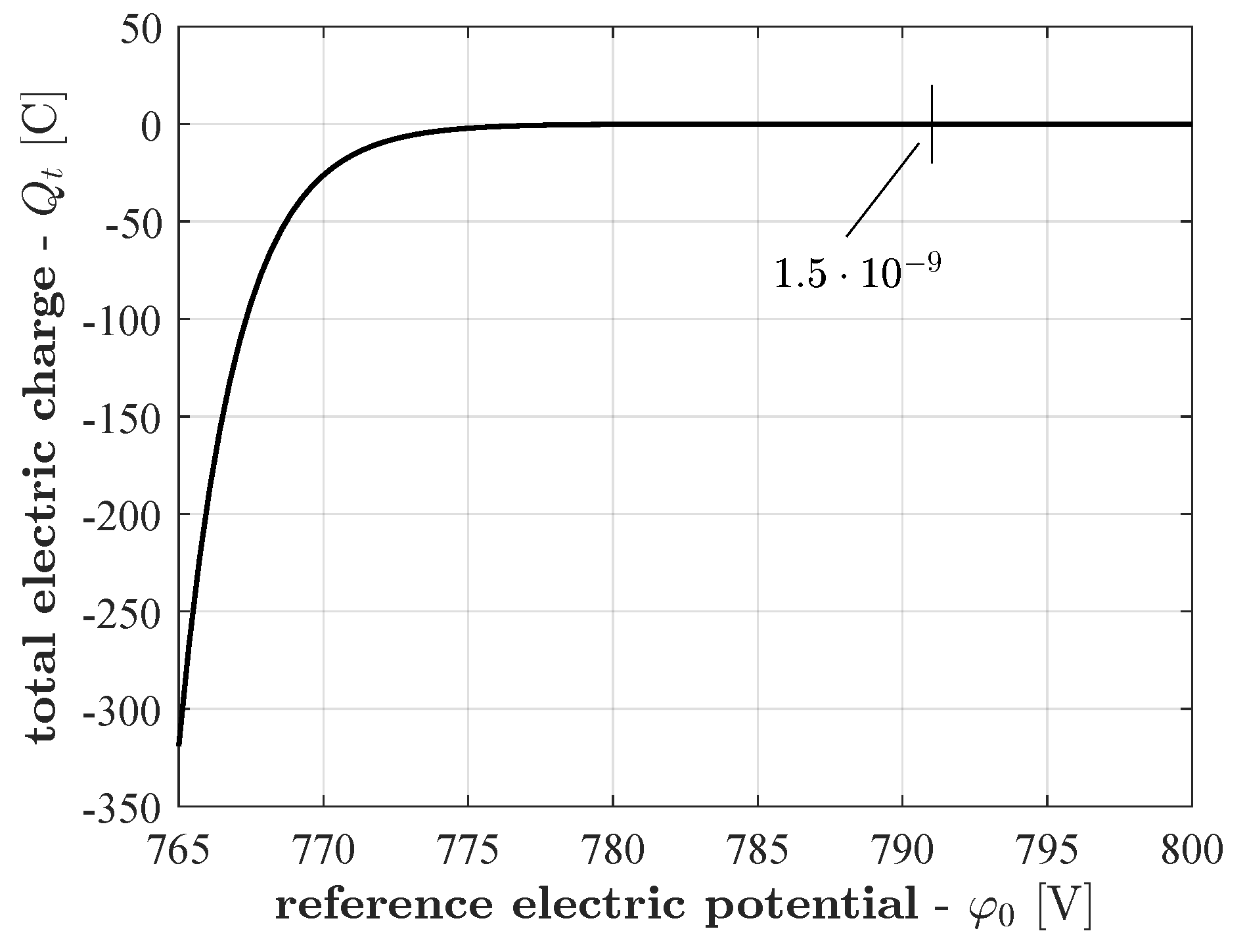
2.4. Charge Conservation

The described non-linear Poisson formulation (12) is not charge-conserving. In other words, there is no guarantee that its solution yields a net negative charge due to the electrons balancing the one due (positive and negative) ions. This is a limitation to be addressed since, in comparison, global charge neutrality is automatically satisfied when a full drift diffusion approach is used, meaning that the drift diffusion approach is also used for electrons (and a linear Poisson problem is solved at each iteration).
We therefore add charge conservation as a constraint for the non-linear problem (12). A given value reference electric potential φ 0 (12) yields a spatial distribution of electrons that can be added to the net charge due to the combination of free ions and surface charge (also influenced by electron fluxes).
Q t = Q i Q e ,
Q i is the total (volume and surface) charge due to ions and is evaluated as:
Q i = k = 1 n nodes ρ i , k Δ V k volume + j = 1 n diel ρ Σ i , j S j surface ,
where ρ i , k = s i q s n s is the volume charge density due to ions and Δ V k is the k-th nodal volume; ρ Σ i , j is the ion surface charge density on the j-th solid dielectric layer, whose area is S j . Similarly, Q e is the total charge due to electrons:
Q e = k = 1 n nodes ρ e , k Δ V k + j = 1 n diel ρ Σ e , j S j
We propose to look at the reference potential φ 0 as a free parameter that can be used to enforce the electric neutrality Q t = 0 . However, finding the particular value of φ 0 that satisfies the electric neutrality is also a nonlinear problem. The obvious way to approach this (second) nonlinearity is to include the condition Q t = 0 within the Newton–Raphson algorithm. However, the way in which Q t depends on φ 0 makes the Newton–Raphson scheme rather unsuitable for solving this problem, particularly when large voltages are considered. Figure 2 shows the total electric charge ( Q t ) as a function of φ 0 when 800 V are applied between the two ends of the considered domain, for the same test problem considered in Figure 1. The Newton–Raphson method is notoriously unsuited to solve problems where the unknown function exhibits near-zero or very steep slopes, and the problem in Figure 2 features both these two critical situations, above and below the zero of the unknown function Q t .
For this reason, instead of directly enforcing Q t = 0 in the Newton–Raphson framework, an iterative procedure based on the bisection method has been developed to solve the described problem in a robust way. The convergence of the bisection method is only linear, but, as opposed to the Newton–Raphson method, unconditionally stable, provided that appropriate initial conditions are provided. In particular, two initial values φ 0 , + and φ 0 , must be provided, yielding a positive and negative value for Q t , respectively, when substituted in (12).
The pseudocode procedure for solving the non-linear Poisson problem based on the bisection method is provided in Algorithm 1. Starting from φ 0 , + and φ 0 , , a tentative reference potential φ 0 is obtained as the midpoint of the interval [ φ 0 , ; φ 0 , + ] . Then, the resulting nonlinear Poisson problem is solved using the Newton–Raphson algorithm. The obtained electron distribution yields a total electric charge Q t , φ 0 . If Q t , φ 0 > 0 , φ 0 becomes φ 0 , + for the next iteration. Otherwise, φ 0 becomes φ 0 , . The cycle continues until | Q t , φ 0 | is lower than the requested tolerance.
Algorithm 1: Non-linear Poisson solver with global charge conservation
Plasma 06 00027 i001
At this point, one is left with the problem of finding the two starting values for the bisection method. Obtaining these values robustly can become somewhat problematic when large voltages that change over time are considered, since the quantity φ φ 0 is the argument of an exponential function in (11).
Algorithm 2 shows the procedure adopted to obtain φ 0 , + and φ 0 , . The starting electric potential distribution ( φ ) for the Newton–Raphson solver is obtained via a linear Poisson problem under the assumption of uniform distribution of the electron number density in the domain. The nonlinear Poisson problem is solved once by setting φ 0 as the maximum value of the previously obtained φ . In this way, the argument of the exponential is ≤0 at the center of each CV. The value of the total electric charge Q t , φ 0 is compared to zero. If Q t , φ 0 > 0 , it means that φ 0 can be used as φ 0 , + for the subsequent bisection cycle, and a value of φ 0 that yields Q t < 0 must be found iteratively. This is performed by progressively lowering φ 0 , in steps corresponding to T e / 5 , where T e is the electron temperature in Volt. The cycle continues until Q t < 0 is obtained, meaning that the employed φ 0 can be used as φ 0 , in the bisection cycle. In contrast, if the starting value of Q t is negative, the value of φ 0 yielding a positive Q t , i.e., φ 0 , + , is iteratively found by increasing φ 0 in steps of T e / 5 .
Algorithm 2: Iterative search of reference electric potential
Plasma 06 00027 i002

3. Simulation Results

In this section, we use the computational model described in Section 2 to simulate the physical behavior of a volumetric DBD reactor when powered by a sinusoidal voltage waveform. We chose this specific reactor topology over, e.g., a surface reactor for two main reasons: first, it can be described in one spatial dimension, allowing for faster simulations. Second, in a surface reactor, one has to deal with an open domain, which makes considerations on charge conservation more complex. The computer program for this work is coded in Fortran 90. We chose this language over more user-friendly interpreted languages such as MATLAB to benefit from the substantial performance speedup resulting from optimizations performed during code compilation, such as vectorization, loop unrolling, or function inlining [52]. Furthermore, Fortran 90 supports both shared-memory and distributed-memory parallel communication protocols, such as OpenMP and MPI. Although explicit multicore processing is supported in MATLAB through the Parallel Computing Toolbox [53], the above tools offer more flexibility and smaller overheads.

3.1. Simulation Settings

The modeled device consists of a closed volumetric DBD reactor consisting of two parallel metal electrodes separated by two dielectric layers with relative permittivity ϵ r = 3.4 , corresponding to Kapton. The thickness of the air gap between the two electrodes is 4 × 10 4   m . Each of the two dielectric layers has a thickness of 2 × 10 4   m and a 1.6 × 10 3 m2 surface. The configuration is powered by a 15 k Hz sinusoidal voltage with amplitude 4.8   k V .
The simulations are carried out using a simplified plasma chemistry model for dry air, with a small amount of species. This model, which consists of 21 reactions, has been developed in [43] by expanding the model proposed by Parent et al. in [54]. The mechanism includes electron impact ionization, two- and three-body recombination, electron attachment, detachments, dissociation, and a simple O3 formation chain; see Table A1. The considered heavy species are N2+, O2+, O2, O, O, and O3. As introduced in Section 2, electrons may or may not be accounted for in the drift diffusion model, depending on the electron model chosen by the user. A numerical validation of the implemented semi-implicit approach for the source term time integration is provided in Appendix A.
Regardless of the absolute abundance of the species at the beginning of the simulation, the initial ratio between N2+ and O2+ is set to 3:1. The O2 is set to a 1:8 ratio with respect to N2+ and the electron density is selected to ensure overall electric neutrality. The macroscopic transport parameters for the considered species have been taken from [54].

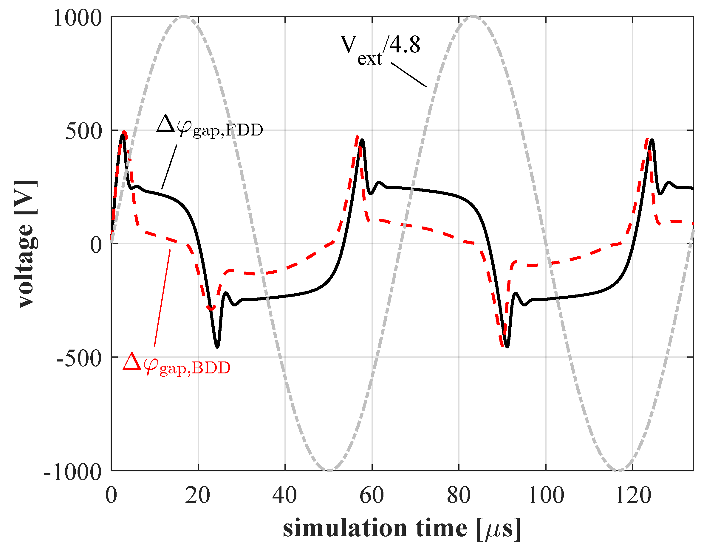
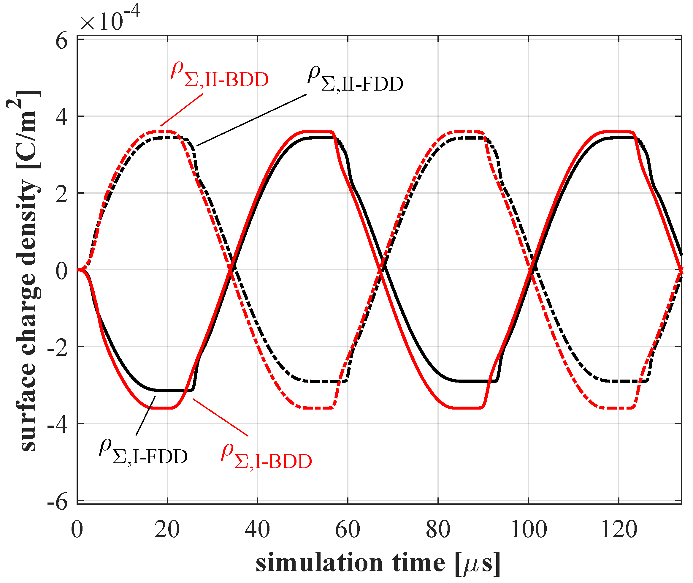
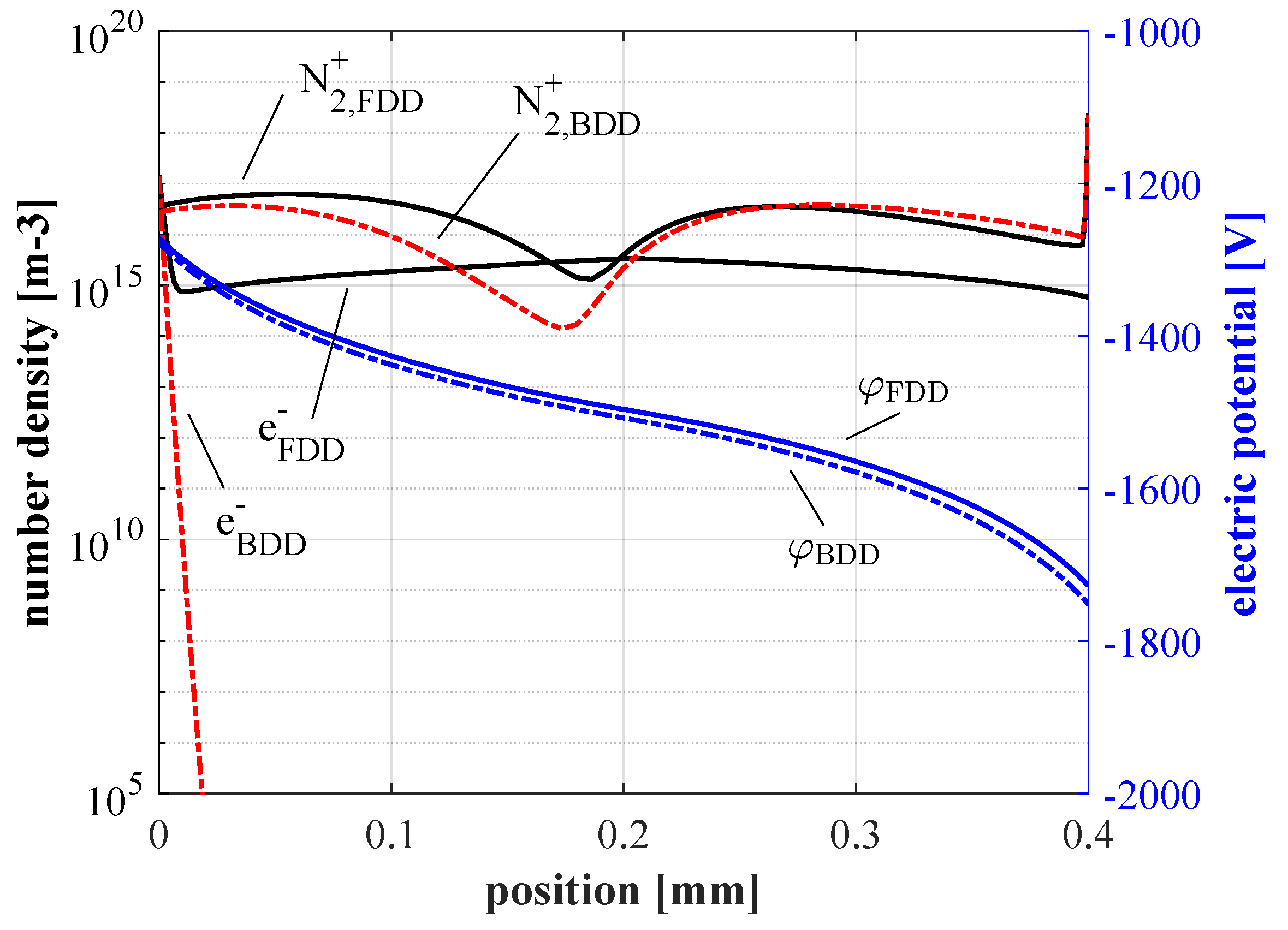
3.2. Electron Models Comparison

The aim of this section is to compare the results obtained using the proposed methodology—where electrons are modeled using the Boltzmann relation—to those yielded by a classic strategy where electrons are included in the drift diffusion approach. The two methodologies will be referred to as Boltzmann drift diffusion (BDD) and full drift diffusion (FDD) from now on for the sake of brevity.
Figure 3 shows the gap voltage ( Δ φ gap ) during the first two cycles of the voltage waveform ( V ext ) applied between the two electrodes. The applied external voltage has been normalized to highlight the differences yielded by the two approaches. The gap voltage is defined by Δ φ gap = φ L φ R , where φ L and φ R are the electric potential values at the left and right ends of the 1-D domain, respectively.
In other words, Δ φ gap is the voltage to which the air gap is effectively subjected. This is in general different from V ext due to the voltage drop across the layers (which depends on the thickness and the relative permittivity ( ϵ r , d ) of the layer) and the combination of the field produced by the volumetric and surface charge density distributions.
The combination of these mechanisms causes Δ φ gap to reach a maximum value of 475 V during the first quarter of the (first) cycle, after 2.5   μ s from the beginning of the simulation. Then, while V ext continues to increase, Δ φ gap starts to decrease, reaching zero in the second quarter.
During the first half of the cycle, negative charges (negative ions and free electrons) drift towards the anode. Similarly, positive ions are pushed towards the opposite electrode, acting as the cathode. Hence, the two dielectric layers (L) and (R) are subjected to a flux of negative and positive charges, respectively.
The two curves marked as Δ φ gap , FDD and Δ φ gap , BDD in Figure 3 correspond to the gap voltages provided by the two methodologies. The results are reasonably close and show the same trend over time. Moreover, the peak values of Δ φ gap become almost coincident after the first half-cycle of the applied voltage. However, from the second quarter of the first cycle, the peaks of Δ φ gap obtained with the FDD method show a time delay of approximately 1 μ s with respect to the results yielded by the BDD method. This is due to the assumption that the electrons instantaneously adapt their spatial distribution according to the Boltzmann relation as a reaction to the external electric field and changes in the ions’ number density. In addition to the small temporal change between the two trends in the gap voltage, the main difference between the two approaches appears to be constituted by the lower Δ φ gap obtained when the BDD methodology is used. This means that the mechanism by which the charged species spontaneously screen out the externally applied electric field is not exactly equal in the two considered cases. The surface charge deposition onto the dielectric layers covering the electrodes is the most important mechanism that contributes to the differences between the applied voltage and the gap voltage. Figure 4 shows the surface charge accumulated on the two layers over the same time period considered in Figure 3. The results obtained by the two approaches are in good qualitative agreement. Still, a difference can be noticed in the negative charging process, mainly due to electrons. In fact, the positive and negative charging fronts yielded by the FDD methodology are slightly asymmetric. In contrast, the positive and negative surface charge deposition dynamics appear to be completely symmetric when the electrons are excluded from the drift diffusion approach (BDD). As a result of this, a larger amount of negative charge is stored in the dielectric layers in this way, exerting a stronger screening effect with respect to the externally applied field, causing the lower values of Δ φ gap shown in Figure 3.
Finally, the number density distribution over the gas gap yielded by the two methodologies after 57.7   μ s from the beginning of the simulation is shown in Figure 5. The results corresponding to the Boltzmann drift diffusion approach have been shifted 0.9   μ s forward in time to compensate for the time delay shown in Figure 3. As one can see, the obtained distribution of heavy ions is comparable over the whole gap. On the contrary, the two electron number density distributions are significantly different. Although the FDD method predicts an approximately uniform number density 1 × 10 15 m 3 in the bulk of the gap, the density yielded by the BDD approach drops below 1 × 10 15 m 3 . Nevertheless, for both species, the values obtained within the sheaths at the edges of the domain are well compatible. In particular, the values of N2+ number density at the right edge of the domain (cathodic side) are N 2 FDD + = 2.43 × 10 18   m 3 and N 2 BDD + = 2.24 × 10 18   m 3 . Similarly, the electron number density values at the left edge (anodic side) of the gap are e FDD = 1.44 × 10 17   m 3 and e BDD = 1.41 × 10 17   m 3 . This agreement is important because the number densities at the two edges of the gap are several orders of magnitude larger than in the bulk for both considered species. This means that, given the dependence of the reaction rates on the number density of the reactants, the largest physical contributions from kinetic processes will likely be generated in these regions. In addition, the charged species fluxes directed towards the walls, responsible for the surface charge accumulation process, are computed using the number density in the CVs shared between the dielectric layers and the gap. Therefore, the discussed agreement between the computed number densities at the edges of the domain is consistent with the compatibility shown by the trends in surface charge over time in Figure 4. In order to have similar incident wall fluxes, a similar electric field at the gap edges must also be present. The right axis in Figure 5 shows the electric potential obtained using the two methodologies. The value yielded by the BDD approach (which depends on the reference electric potential ϕ 0 ) has been shifted by a constant value of 410 V to allow comparison to φ FDD . The two obtained electric potentials are very close throughout the whole gap, meaning that the two electric fields will also be quite similar to each other.

Computational Performance

Using the BDD technique, the minimum length of the employed time steps is typically increased by 2–3 orders of magnitude. The effective speedup yielded by the BDD approach over the FDD is considerably smaller because the BDD methodology requires multiple solutions of the linear system arising for the computation of the electric potential distribution. The effective speedup, which can vary depending on the number of iterations required to meet the convergence criteria, is generally in the order of 30–50. Because of this, multidimensional simulations of relatively long timescales (such as multiple periods of applied voltages in the kHz range) can be carried out in reasonable times [43].

4. Conclusions

In this work, we presented a computational fluid model dedicated to the description of the dynamics of neutral and charged species in nonthermal plasmas at atmospheric pressure. We focused on the development of a technique allowing to significantly reduce the computational load of these kinds of simulations. The proposed methodology is based on avoiding direct time integration of electron fluxes by relating the electron number density distribution and the local electric potential through the Boltzmann relation. While this approach is well established for problems with low pressure and open boundaries, e.g., space plasma propulsion, we discussed the treatment of the nonlinear electrostatic formulation for closed domains with accumulation of surface charge density over time. We proposed an algorithm for the dynamic adjustment of the reference electric potential appearing in the Boltzmann relation to simultaneously ensure global charge conservation and convergence of the iterative procedure for the electric potential calculation. The proposed Boltzmann drift diffusion methodology was applied to a volumetric DBD reactor powered by a 4.8   kV sinusoidal voltage at 15 kHz . We used the developed methodology to compute the effective voltage applied to the gap and the surface discharge over two cycles of the applied waveform. We compared these results to those obtained when using a full drift diffusion approach, i.e., when the electron number density is updated over time using the drift and diffusion approach in the same way as the ions. The results obtained with the two approaches are in good agreement, particularly concerning the fluxes at walls and the electric field. Overall, considering the substantial advantage in terms of computation time over a full drift diffusion approach, we conclude that the proposed methodology can be successfully applied to the simulation of such discharges.

Author Contributions

Conceptualization, A.P. and A.C.; methodology, A.P. and A.C.; software, A.P.; validation, A.P. and G.N.; formal analysis, A.P. and A.C.; investigation, A.P.; resources, A.C. and G.N.; data curation, A.P.; writing—original draft preparation, A.P. and F.R.; writing—review and editing, A.P., A.C., F.R., G.P. and G.N.; visualization, A.P.; supervision, A.P. and A.C.; project administration, A.P., A.C. and G.N.; funding acquisition, A.C. and G.N. All authors have read and agreed to the published version of the manuscript.

Funding

This research received no external funding.

Institutional Review Board Statement

Not applicable.

Informed Consent Statement

Not applicable.

Data Availability Statement

The data presented in this study are available upon reasonable request to the authors.

Conflicts of Interest

The authors declare no conflict of interest.

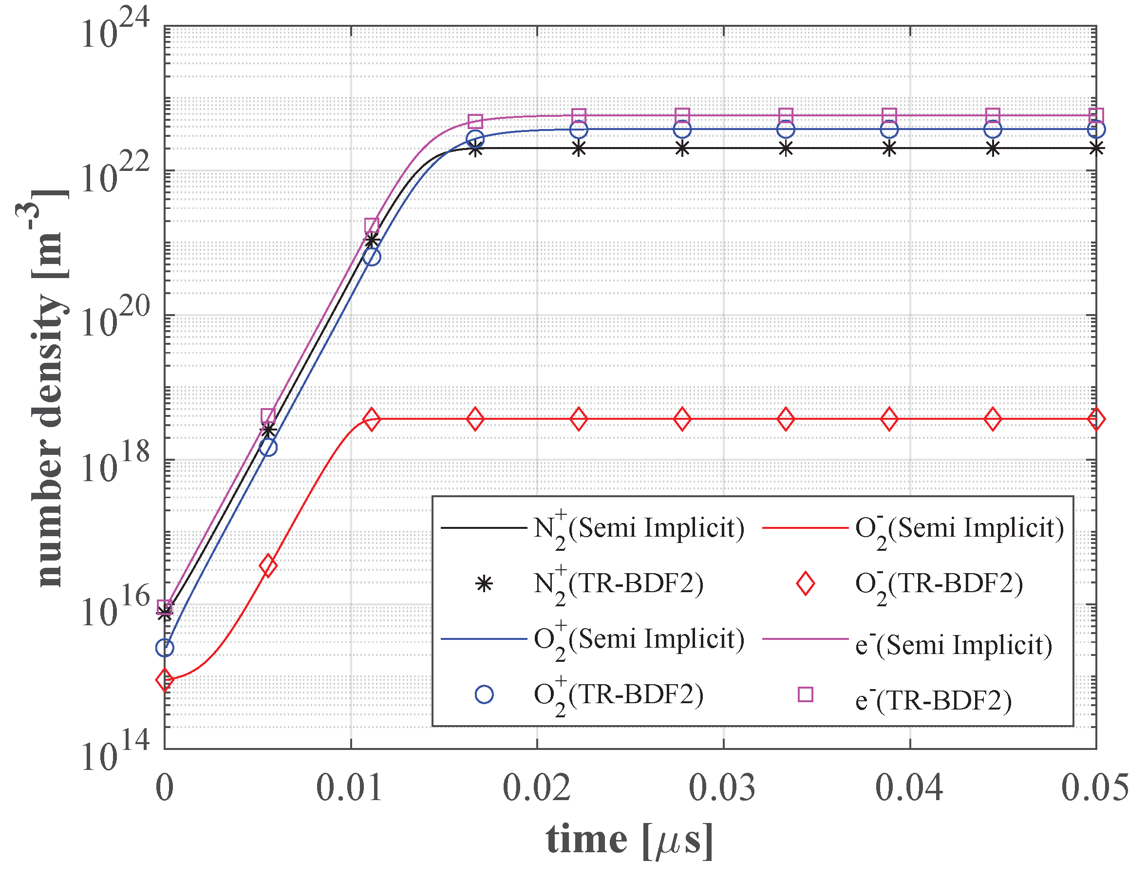
Appendix A. Numerical Validation of the Semi-Implicit Source Term Integrator

The semi-implicit scheme employed for the integration of the source terms in the RHS of the conservation equation has been tested against the well-established TR-BDF2 scheme. The TR-BDF2 method is an implicit scheme, employing a combination of a trapezoidal rule and backwards differentiation [55]. The considered reactions are the ones corresponding to Ref. [54] in Table A1. A constant electric field of 160 Td has been applied over a timespan of 0.05   μ s . The results of the comparison are summarized in Figure A1. The species are followed over a time interval Δ t considerably larger than the time steps typical of explicit simulations, which are usually in the pico-second range (or even smaller). This choice was purposely made to test the accuracy of the semi-implicit scheme under particularly restrictive conditions. The initial number densities at time t 0 = 0   s of the considered species are N 2 + | t 0 = 0.75 · n 0 , O 2 + | t 0 = 0.25 · n 0 , O 2 | t 0 = 0.09 · n 0 , e | t 0 = 0.91 · n 0 , where n 0 = 1 × 10 16   m 3 . For what concerns the neutral species, their initial number densities have been set to N 2 | t 0 = 0.75 · 2.686 × 10 25   m 3 and O 2 | t 0 = 0.25 · 2.686 × 10 25   m 3 , respectively.
Table A1. List of considered kinetic processes, along with the relevant reference.
ProcessReactants Product(s)Source
IonizationN2 + eN2+ + 2e[54]
O2 + eO2+ + 2e[54]
RecombinationN2+ + eN2[54]
O2+ + eO2[54]
N2+ + O2N2 + O2[54]
O2+ + O22O2[54]
N2 + N2+ + O22N2 + O2[54]
N2 + O2+ + O2N2 + 2O2[54]
O2 + N2+ + O2N2 + O2 + O2 e[54]
O2 + O2+ + O2O2 + O2 + O2[54]
AttachmentN2 + O2 + eN2 + O2[54]
O2 + O2 + eO2 + O2[54]
O2 + O + eO2 + O[56]
O3 + eO2 + O[56]
O3 + eO2 + O[56]
DetachmentO2 + O2O2 + O2 + e[54]
O2 + OO3 + e[56]
DissociationO2 + eO + O + e[56]
O3 + eO2 + O + e[56]
O3 formationO + O2 + N2 O3 + N2[56]
O + O2 + O2O3 + O2[56]
Figure A1. Comparison between the described semi-implicit numerical scheme and the TR-BDF2 [55] integration method. Time evolution of the charged species considered in [54], with | E | = 200   Td .
Plasma 06 00027 g0a1
The results of the described comparison are shown in Figure A1. Continuous lines are employed in the picture to indicate the results obtained with the semi-implicit methodology, while markers of matching colors are used for the TR-BDF2 method. The results obtained using the semi-implicit technique are in close agreement with the ones yielded by the TR-BDF2 routine. The highest relative percent difference between the two approaches, obtained for the O 2 number density, is 1.03 %.
An important requirement that must be respected in the source terms integration process is the conservation of the total electric charge. With reference to the test depicted in Figure A1, the initial number densities have been selected to yield a null initial electric charge density ( ρ 0 = 0 ). The latter can be obtained summing the product of each species number density and charge, as in:
ρ = s N s n s q s ,
where N s is the total number of considered species. The net charge density (normalized to n 0 and to the elementary charge q e ) obtained at the end of the integration time with the semi-implicit methodology is ρ s i = 2.6 × 10 13 . The same quantity obtained at the end of the adopted timespan with the TR-BDF2 was ρ T R B D F 2 = 1.76 × 10 5 . Hence, the proposed semi-implicit methodology appears to better preserve the global charge neutrality of the species involved in the kinetic processes.

References

  1. Neretti, G.; Popoli, A.; Scaltriti, S.G.; Cristofolini, A. Real Time Power Control in a High Voltage Power Supply for Dielectric Barrier Discharge Reactors: Implementation Strategy and Load Thermal Analysis. Electronics 2022, 11, 1536. [Google Scholar] [CrossRef]
  2. Kogelschatz, U. Atmospheric-pressure plasma technology. Plasma Phys. Control. Fusion 2004, 46, B63–B75. [Google Scholar] [CrossRef]
  3. Monrolin, N.; Plouraboué, F. Multi-scale two-domain numerical modeling of stationary positive DC corona discharge/drift-region coupling. J. Comput. Phys. 2021, 443, 110517. [Google Scholar] [CrossRef]
  4. Belinger, A.; Dap, S.; Naudé, N. Influence of the dielectric thickness on the homogeneity of a diffuse dielectric barrier discharge in air. J. Phys. D Appl. Phys. 2022, 55, 465201. [Google Scholar] [CrossRef]
  5. Shang, J.S.; Huang, P.G. Surface plasma actuators modeling for flow control. Prog. Aerosp. Sci. 2014, 67, 29–50. [Google Scholar] [CrossRef]
  6. Adamiak, K. Quasi-stationary modeling of the DBD plasma flow control around airfoil. Phys. Fluids 2020, 32, 085108. [Google Scholar] [CrossRef]
  7. Adamiak, K. Approximate Formulations in Mean Models of Dielectric Barrier Discharge Plasma Flow Actuator. AIAA J. 2022, 60, 4215–4226. [Google Scholar] [CrossRef]
  8. Li, S.; Dang, X.; Yu, X.; Abbas, G.; Zhang, Q.; Cao, L. The application of dielectric barrier discharge non-thermal plasma in VOCs abatement: A review. Chem. Eng. J. 2020, 388, 124275. [Google Scholar] [CrossRef]
  9. Nayak, G.; Simeni Simeni, M.; Rosato, J.; Sadeghi, N.; Bruggeman, P. Characterization of an RF-driven argon plasma at atmospheric pressure using broadband absorption and optical emission spectroscopy. J. Appl. Phys. 2020, 128, 243302. [Google Scholar] [CrossRef]
  10. Jenns, K.; Sassi, H.; Zhou, R.; Cullen, P.; Carter, D.; Mai-Prochnow, A. Inactivation of foodborne viruses: Opportunities for cold atmospheric plasma. Trends Food Sci. Technol. 2022, 124, 323–333. [Google Scholar] [CrossRef]
  11. Massima Mouele, E.S.; Tijani, J.O.; Badmus, K.O.; Pereao, O.; Babajide, O.; Zhang, C.; Shao, T.; Sosnin, E.; Tarasenko, V.; Fatoba, O.O.; et al. Removal of Pharmaceutical Residues from Water and Wastewater Using Dielectric Barrier Discharge Methods—A Review. Int. J. Environ. Res. Public Health 2021, 18, 1683. [Google Scholar] [CrossRef]
  12. Guo, H.; Su, Y.; Yang, X.; Wang, Y.; Li, Z.; Wu, Y.; Ren, J. Dielectric Barrier Discharge Plasma Coupled with Catalysis for Organic Wastewater Treatment: A Review. Catalysts 2023, 13, 10. [Google Scholar] [CrossRef]
  13. Feizollahi, E.; Misra, N.; Roopesh, M.S. Factors influencing the antimicrobial efficacy of Dielectric Barrier Discharge (DBD) Atmospheric Cold Plasma (ACP) in food processing applications. Crit. Rev. Food Sci. Nutr. 2021, 61, 666–689. [Google Scholar] [CrossRef]
  14. Seri, P.; Nici, S.; Cappelletti, M.; Scaltriti, S.G.; Popoli, A.; Cristofolini, A.; Neretti, G. Validation of an indirect nonthermal plasma sterilization process for disposable medical devices packed in blisters and cartons. Plasma Process. Polym. 2023, e2300012. [Google Scholar] [CrossRef]
  15. Colonna, G.; Pintassilgo, C.D.; Pegoraro, F.; Cristofolini, A.; Popoli, A.; Neretti, G.; Gicquel, A.; Duigou, O.; Bieber, T.; Hassouni, K.; et al. Theoretical and experimental aspects of non-equilibrium plasmas in different regimes: Fundamentals and selected applications. Eur. Phys. J. D 2021, 75, 183. [Google Scholar] [CrossRef]
  16. Lu, X.; Bruggeman, P.; Reuter, S.; Naidis, G.; Bogaerts, A.; Laroussi, M.; Keidar, M.; Robert, E.; Pouvesle, J.M.; Liu, D.; et al. Grand challenges in low temperature plasmas. Front. Phys. 2022, 10, 28–36. [Google Scholar] [CrossRef]
  17. Roth, M.; Schollmeier, M. Ion Acceleration—Target Normal Sheath Acceleration. CERN Yellow Rep. 2016, 1, 231–270. [Google Scholar] [CrossRef]
  18. Golubovskii, Y.B.; Maiorov, V.A.; Behnke, J.; Behnke, J.F. Modelling of the homogeneous barrier discharge in helium at atmospheric pressure. J. Phys. D Appl. Phys. 2002, 36, 39. [Google Scholar] [CrossRef]
  19. Tochikubo, F.T.F.; Chiba, T.C.T.; Watanabe, T.W.T. Structure of Low-Frequency Helium Glow Discharge at Atmospheric Pressure between Parallel Plate Dielectric Electrodes. Jpn. J. Appl. Phys. 1999, 38, 5244. [Google Scholar] [CrossRef]
  20. Becker, K.H.; Kogelschatz, U.; Schoenbach, K.; Barker, R. Non-Equilibrium Air Plasmas at Atmospheric Pressure; CRC Press: Boca Raton, FL, USA, 2004. [Google Scholar]
  21. Shaygani, A.; Adamiak, K. Mean model of the dielectric barrier discharge plasma actuator including photoionization. J. Phys. Appl. Phys. 2023, 56, 055203. [Google Scholar] [CrossRef]
  22. Sato, S.; Shiroto, T.; Takahashi, M.; Ohnishi, N. A fast solver of plasma fluid model in dielectric-barrier-discharge simulation. Plasma Sources Sci. Technol. 2020, 29, 075007. [Google Scholar] [CrossRef]
  23. Nakai, K.; Komuro, A.; Nishida, H. Effect of chemical reactions on electrohydrodynamic force generation process in dielectric barrier discharge. Phys. Plasmas 2020, 27, 063518. [Google Scholar] [CrossRef]
  24. Hua, W.; Fukagata, K. Near-surface electron transport and its influence on the discharge structure of nanosecond-pulsed dielectric-barrier-discharge under different electrode polarities. Phys. Plasmas 2019, 26, 013514. [Google Scholar] [CrossRef]
  25. Sato, S.; Furukawa, H.; Komuro, A.; Takahashi, M.; Ohnishi, N. Successively accelerated ionic wind with integrated dielectric-barrier-discharge plasma actuator for low-voltage operation. Sci. Rep. 2019, 9, 5813. [Google Scholar] [CrossRef] [PubMed] [Green Version]
  26. Emmons, D.J.; Weeks, D.E. Steady-State Model of an Argon-Helium High-Pressure Radio Frequency Dielectric Barrier Discharge. IEEE Trans. Plasma Sci. 2020, 48, 2715–2722. [Google Scholar] [CrossRef]
  27. Zhong, L.; Wu, B.; Wang, Y. Low-temperature plasma simulation based on physics-informed neural networks: Frameworks and preliminary applications. Phys. Fluids 2022, 34, 087116. [Google Scholar] [CrossRef]
  28. Zhang, Y.T.; Gao, S.H.; Ai, F. Efficient numerical simulation of atmospheric pulsed discharges by introducing deep learning. Front. Phys. 2023, 11, 1125548. [Google Scholar] [CrossRef]
  29. Boeuf, J.P.; Lagmich, Y.; Unfer, T.; Callegari, T.; Pitchford, L.C. Electrohydrodynamic force in dielectric barrier discharge plasma actuators. J. Phys. D Appl. Phys. 2007, 40, 652. [Google Scholar] [CrossRef]
  30. Cristofolini, A.; Popoli, A. A multi-stage approach for DBD modelling. J. Phys. Conf. Ser. 2019, 1243, 012012. [Google Scholar] [CrossRef]
  31. Boeuf, J.P.; Merad, A. Fluid and Hybrid Models of Non Equilibrium Discharges. In Plasma Processing of Semiconductors; Williams, P.F., Ed.; Springer: Dordrecht, The Netherlands, 1997; pp. 291–319. [Google Scholar] [CrossRef]
  32. Ventzek, P.L.G.; Sommerer, T.J.; Hoekstra, R.J.; Kushner, M.J. Two-dimensional hybrid model of inductively coupled plasma sources for etching. Appl. Phys. Lett. 1993, 63, 605–607. [Google Scholar] [CrossRef] [Green Version]
  33. Ventzek, P.L.G.; Hoekstra, R.J.; Kushner, M.J. Two-dimensional modeling of high plasma density inductively coupled sources for materials processing. J. Vac. Sci. Technol. B Microelectron. Nanometer Struct. Process. Meas. Phenom. 1994, 12, 461–477. [Google Scholar] [CrossRef]
  34. Punset, C.; Cany, S.; Boeuf, J.P. Addressing and sustaining in alternating current coplanar plasma display panels. J. Appl. Phys. 1999, 86, 124–133. [Google Scholar] [CrossRef]
  35. Lin, K.M.; Hung, C.T.; Hwang, F.N.; Smith, M.; Yang, Y.W.; Wu, J.S. Development of a parallel semi-implicit two-dimensional plasma fluid modeling code using finite-volume method. Comput. Phys. Commun. 2012, 183, 1225–1236. [Google Scholar] [CrossRef]
  36. Teunissen, J. Improvements for drift-diffusion plasma fluid models with explicit time integration. Plasma Sources Sci. Technol. 2020, 29, 015010. [Google Scholar] [CrossRef] [Green Version]
  37. Tamura, H.; Sato, S.; Ohnishi, N. Numerical simulation of atmospheric-pressure surface dielectric barrier discharge on a curved dielectric with a curvilinear mesh. J. Phys. D Appl. Phys. 2022, 56, 045202. [Google Scholar] [CrossRef]
  38. Kwok, D.T.K. A hybrid Boltzmann electrons and PIC ions model for simulating transient state of partially ionized plasma. J. Comput. Phys. 2008, 227, 5758–5777. [Google Scholar] [CrossRef]
  39. Holgate, J.T.; Coppins, M. Numerical implementation of a cold-ion, Boltzmann-electron model for nonplanar plasma-surface interactions. Phys. Plasmas 2018, 25, 043514. [Google Scholar] [CrossRef] [Green Version]
  40. Cartwright, K.L.; Verboncoeur, J.P.; Birdsall, C.K. Nonlinear hybrid Boltzmann—Particle-in-cell acceleration algorithm. Phys. Plasmas 2000, 7, 3252–3264. [Google Scholar] [CrossRef]
  41. Kang, S.H. PIC-DSMC Simulation of a Hall Thruster Plume with Charge Exchange Effects Using pdFOAM. Aerospace 2023, 10, 44. [Google Scholar] [CrossRef]
  42. Brieda, L. Plasma Simulations by Example, 1st ed.; CRC Press: Boca Raton, FL, USA, 2019. [Google Scholar]
  43. Cristofolini, A.; Popoli, A.; Neretti, G. A multi-stage model for dielectric barrier discharge in atmospheric pressure air. Int. J. Appl. Electromagn. Mech. 2020, 63, S21–S29. [Google Scholar] [CrossRef]
  44. Lieberman, M.A.; Lichtenberg, A.J. Principles of Plasma Discharges and Materials Processing, 2nd ed.; John Wiley & Sons, Inc.: Hoboken, NJ, USA, 2005. [Google Scholar]
  45. LeVeque, R.J. Finite Volume Methods for Hyperbolic Problems; Cambridge University Press: Cambridge, UK, 2002; Volume 31. [Google Scholar]
  46. Hirsch, C. Numerical Computation of Internal and External Flows: The Fundamentals of Computational Fluid Dynamics; John Wiles & Sons: Chichester, UK, 1988; Volume 1. [Google Scholar]
  47. Scharfetter, D.; Gummel, H. Large-signal analysis of a silicon Read diode oscillator. IEEE Trans. Electron Devices 1969, 16, 64–77. [Google Scholar] [CrossRef]
  48. Kulikovsky, A.A. A More Accurate Scharfetter-Gummel Algorithm of Electron Transport for Semiconductor and Gas Discharge Simulation. J. Comput. Phys. 1995, 119, 149–155. [Google Scholar] [CrossRef]
  49. Liu, L.; van Dijk, J.; ten Thije Boonkkamp, J.H.M.; Mihailova, D.B.; van der Mullen, J.J.A.M. The complete flux scheme—Error analysis and application to plasma simulation. J. Comput. Appl. Math. 2013, 250, 229–243. [Google Scholar] [CrossRef]
  50. Nguyen, T.D.; Besse, C.; Rogier, F. High-order Scharfetter-Gummel-based schemes and applications to gas discharge modeling. J. Comput. Phys. 2022, 461, 111196. [Google Scholar] [CrossRef]
  51. Chen, F.F. Introduction to Plasma Physics and Controlled Fusion, 3rd ed.; Springer: Cham, Switzerland, 2016. [Google Scholar]
  52. Metcalf, M.; Reid, J.; Cohen, M. Modern Fortran Explained: Incorporating Fortran 2018; Oxford University Press: Oxford, UK, 2018. [Google Scholar]
  53. Sharma, G.; Martin, J. MATLAB®: A Language for Parallel Computing. Int. J. Parallel Program. 2009, 37, 3–36. [Google Scholar] [CrossRef] [Green Version]
  54. Parent, B.; Macheret, S.O.; Shneider, M.N. Electron and ion transport equations in computational weakly-ionized plasmadynamics. J. Comput. Phys. 2014, 259, 51–69. [Google Scholar] [CrossRef]
  55. Hosea, M.; Shampine, L. Analysis and implementation of TR-BDF2. Appl. Numer. Math. 1996, 20, 21–37. [Google Scholar] [CrossRef]
  56. Kossyi, I.A.; Kostinsky, A.Y.; Matveyev, A.A.; Silakov, V.P. Kinetic scheme of the non-equilibrium discharge in nitrogen-oxygen mixtures. Plasma Sources Sci. Technol. 1992, 1, 207–220. [Google Scholar] [CrossRef]
Figure 1. Solution of the non-linear Poisson problem (12) over a 5 m m domain, with a uniform ions number density φ 0 = 0   V and boundary conditions φ L = 5   V and φ R = 5   V .
Plasma 06 00027 g001
Figure 2. Total electric charge dependence from the employed reference electric potential; the target value of Q t meeting the required charge neutrality condition, highlighted.
Plasma 06 00027 g002
Figure 3. Simulation of the volumetric dielectric barrier discharge reactor with two different numerical methodologies; comparison between the gap voltage obtained with the full drift diffusion (FDD) and Boltzmann drift diffusion (BDD) approaches.
Plasma 06 00027 g003
Figure 4. Surface charge density deposited onto dielectric layers I and II over two cycles of the externally applied voltage; comparison between the full drift diffusion (FDD, black line) and Boltzmann Drift diffusion (BDD, red line) approaches.
Plasma 06 00027 g004
Figure 5. Spatial distribution of N2+ and e (left) and electric potential (right) yielded by the full drift diffusion (FDD, solid lines) and Boltzmann drift diffusion (BDD, dashed lines) approaches at τ = 57   μ s .
Plasma 06 00027 g005
Disclaimer/Publisher’s Note: The statements, opinions and data contained in all publications are solely those of the individual author(s) and contributor(s) and not of MDPI and/or the editor(s). MDPI and/or the editor(s) disclaim responsibility for any injury to people or property resulting from any ideas, methods, instructions or products referred to in the content.

