A Supersensitive Method for Spectroscopic Diagnostics of Electrostatic Waves in Magnetized Plasmas

Abstract

For relatively strong magnetic fields, hydrogen atoms can have delocalized bound states of almost macroscopic dimensions. Therefore, such states are characterized by a Giant Electric Dipole Moment (GEDM), thus making them very sensitive to an external electric field. We considered the manifestations of the GEDM states in hydrogen spectral line profiles in the presence of a quasimonochromatic electrostatic wave of a frequency ω in a plasma. We demonstrated that in this situation, hydrogen spectral lines can exhibit quasi-satellites, which are the envelopes of Blochinzew-type satellites. We showed that the distinctive feature of such quasi-satellites is that their peak intensity is located at the same distance from the line center (in the frequency scale) for all hydrogen spectral lines, the distance being significantly greater than the wave frequency ω. At the absence of the GEDM (and for relatively strong electrostatic waves), the maxima of the satellite envelopes would be at different distances from the line center for different hydrogen lines. We demonstrated that this effect would constitute a supersensitive diagnostic method for measuring the amplitude of electrostatic waves in plasmas down to ~10 V/cm or even lower.

1. Introduction

There are numerous methods for spectroscopic diagnostics of plasmas (see, e.g., books [1,2,3,4,5,6,7,8,9,10,11] listed in chronological order). Among these methods are those designed for spectroscopic diagnostics of various electrostatic waves in plasmas (see, e.g., books [3,10,11]). These methods, based on the shape of spectral lines of atoms and ions, cover the range of amplitudes of the electrostatic waves from ~1 kV/cm to ~1 GV/cm. In the present paper we describe a possibility to extend the sensitivity of such methods to ~10 V/cm or even lower, as follows.

There are plenty of studies showing that for hydrogenic atoms/ions in a uniform magnetic field, the center-of-mass motion and the relative (internal) motion are coupled by the magnetic field and, rigorously speaking, cannot be separated (see, e.g., papers [12,13,14] and references therein). A pseudoseparation is possible for hydrogen atoms. It leads to a Hamiltonian for the relative motion that depends on a center-of-mass integral of the motion K called pseudomomentum but does not depend on the center-of-mass coordinate [14]. We remind that the pseudomomentum K is the canonical variable conjugated to the center-of-mass coordinate.

A diamagnetic potential term in the Hamiltonian for the relative motion is responsible for the formation of an additional potential well far away from the hydrogen nucleus (proton). For relatively strong magnetic fields, the new bound states inside this well are delocalized states of almost macroscopic dimensions. Therefore, the bound state inside this well is characterized by a Giant Electric Dipole Moment (GEDM), thus making such states very sensitive to an external electric field.

In the present paper we consider the effect of a quasimonochromatic electrostatic wave of a frequency ω in a plasma on hydrogen spectral lines in the presence of the GEDM states. We show that, in this situation, hydrogen spectral lines can exhibit quasi-satellites. The quasi-satellites are envelopes of Blochinzew-type satellites [15], the latter being separated from the line center by multiples of the wave frequency ω (in the frequency scale) in both the red and blue wings. We demonstrated that the distinctive feature of such quasi-satellites (in the presence of the GEDM states) is that their peak intensity is located at the same distance from the line center (in the frequency scale) for all hydrogen spectral lines, the distance being significantly greater than the wave frequency ω. We showed that this effect would allow measuring the amplitude of electrostatic waves in plasmas down to ~10 V/cm or even lower. We provided an example for the conditions of edge plasmas of tokamaks.

2. Materials and Methods

We used the analytical method for finding roots of a cubic polynomial, and no materials were used.

3. Results

In the Hamiltonian of the relative (internal) motion for the hydrogen atom in a magnetic field B, the potential energy has the form (see, e.g., Schmelcher–Cederbaum paper [16], Equation (6))

V = [e²/(2Mc²)]B × r − [|e|/(Mc)](B × K)r − e²/r,

(1)

where K is the pseudomomentum, M is the mass of the hydrogen atom, c is the speed of light, and e is the electron charge. We followed paper [16] in choosing e < 0; we also note that in paper [16] it was set at c = 1. In Equation (1), (B × K)r stands for the scalar product (also known as the dot-product) of vector r and vector (B × K).

We also assumed the same configuration as chosen in paper [16]: B = (0, 0, B) and K = (0, K, 0), where K > 0. Then, Equation (1) takes the form:

V = [e²B²/(2Mc²)](x² + y²) + [|e|BK/(Mc)]x − e²/(x² + y² + z²)^1/2.

(2)

For simplifying equations, we introduce the following scaled potential energy V_s:

V_s = Mc²V/(e²B²).

(3)

Then, Equation (2) can be rewritten as follows:

V_s = (x² + y²)/2 + [Kc/(|e|B)]x − Mc²/[B²(x² + y² + z²)^1/2].

(4)

By equating partial derivatives of vs. with respect to y and z to zeros, we found that this occurred at y = z = 0 (as in paper [16]). The partial derivative of vs. with respect to x that we calculated for finding extrema of the potential had the form:

∂V_s/∂x = x + Kc/(|e|B) + Mc²x/[B²(x² + y² + z²)^3/2].

(5)

At y = z = 0, Equation (5) becomes:

∂V_s/∂x = x + Kc/(|e|B) + (Mc²/B²) (sign x)/x².

(6)

We remind that sign x = 1 for x > 0 or sign x = −1 for x < 0.

On equating ∂V_s/∂x from Equation (6) to zero, we arrived at the following equation:

x³ + [Kc/(|e|B)]x² + (Mc²/B²)(sign x) = 0.

(7)

Thus, for x > 0 and for x < 0, Equation (7) leads to two different equations.

For x > 0, Equation (7) becomes:

x³ + [Kc/(|e|B)]x² x² + (Mc²/B²) = 0.

(8)

Obviously, Equation (8) does not have positive roots.

For x < 0, Equation (7) leads to

|x|³ − [Kc/(|e|B)]|x|² + (Mc²/B²) = 0.

(9)

Equation (9) is equivalent to Equation (8b) from paper [16]; we remind that in paper [16] it was set to c = 1 and e = −1.

The polynomial in Equation (9) has either two or zero real roots. Thus, the total number of roots of Equation (7) is also either two or zero since there are no positive roots.

We note in passing that the authors of paper [16] erroneously stated that ∂V/∂x, calculated at y = z = 0, can have three real roots. Their error originates from the fact that they missed the factor (sign x) in the corresponding equation.

We introduce the scaled magnetic field b and the scaled pseudomomentum k, as follows

b = B/(cM^1/2), k = K/(|e|M^1/2),

(10)

where b has the dimension of cm^−3/2 and k has the dimension of cm^−1/2. Below, while using particular numerical values of b and k, we omit the dimensions for brevity.

With these notations, Equation (9) simplifies as follows:

|x|³ − (k/b)|x|² + 1/b² = 0.

(11)

The discriminant Δ of this cubic equation is

Δ = (4k³ − 27b)/b⁵.

(12)

Therefore, Equation (11) has two distinct real negative roots if Δ > 0, i.e., if

k > 3(b/4)^1/3.

(13)

The exact analytical results for the two real roots x₁ and x₂ of Equation (11) are as follows:

x1 = −k/(3b) − (1 + 31/2i) k2/{22/33b [27b − 2k3 + 33/2(27b2 − 4k3b)1/2]1/3} −
(1 − 31/2i) [27b − 2k3 + 33/2(27b2 − 4k3b)1/2]1/3/(21/36b).

(14)

x₂ = −k/(3b) − (1 − 3^1/2i) k²/{2^2/33b[27b − 2k³ + 3^3/2(27b² − 4k³b)^1/2]^1/3} −
(1 + 3^1/2i) [27b − 2k³ + 3^3/2(27b² − 4k³b)^1/2]^1/3/(2^1/36b).

(15)

It should be emphasized that, despite the presence of the imaginary unit i in Equations (14) and (15), they yield real numbers for x₁ and x₂ under the condition (13).

Figure 1 shows the plot of the root x₁ (solid line) and x₂ (dashed line) versus the scaled magnetic field b for the scaled pseudomomentum k = 10 (corresponding to K = 0.031 a.u. = 6.2 × 10⁻²¹ g cm/s). It is seen that the largest (by the absolute value) root is x₁.

It is easy to find out that, at x = x_1, one has ∂²V_s/∂x² > 0, so that the scaled potential energy vs. has a minimum at x = x₁ (under condition (13)). At x = x₂ one has ∂²V_s/∂x² < 0, so that the scaled potential energy vs. has a maximum at x = x₂ (under condition (13)).

The scaled potential energy vs. at y = z = 0 has the form:

V_s = x²/2 + kx/b − 1/(b²|x|).

(16)

Figure 2 shows the plot of the scaled potential energy vs. from Equation (16) versus the coordinate x (in cm) at the scaled magnetic field b = 1.3 × 10⁶ (corresponding to B = 5 Tesla) for the following three values of the scaled pseudomomentum: k = 400 corresponding to K = 1.25 a.u. (solid line), k = 206 corresponding to K = 0.64 a.u. (dashed line), and k = 100 corresponding to K = 0.31 a.u. (dotted line). These three values of k correspond to the values of the discriminant in Equation (12) Δ > 0, Δ = 0, and Δ < 0, respectively. It is seen that for k = 400, the plot shows a maximum and minimum at x < 0; for k = 206, the plot exhibits a flat part caused by the merging of the maximum and minimum; for k = 100, the plot does not have any extrema, all of this being consistent with the above analytical results.

Figure 3 presents the dependence of the location of the additional potential well x₁ (in cm) on the scaled magnetic field b and on the scaled pseudomomentum k in some ranges of these two parameters. It is seen that |x₁| can reach “macroscopic” values, resulting in a GEDM of such state.

Schmelcher and Cederbaum, in their paper [16], gave only the following approximate formula for x₁ (converted below into our notations):

x_1,CS = −k/b + k/(k³ − 2b).

(17)

As an example, Figure 4 presents the ratio of the approximate root x_1,CS from paper [16] to the exact root x₁ for the scaled pseudomomentum k = 20. It is seen that, for a given k, the relative error of the approximate Formula (17) from paper [16] grows bigger as the scaled magnetic field b increases.

Now let us discuss the corresponding profiles S(w) of hydrogen spectral lines in a magnetized plasma containing an electrostatic wave Fcosωt that propagates perpendicularly to the magnetic field B. Here,

w = Δω/ω

(18)

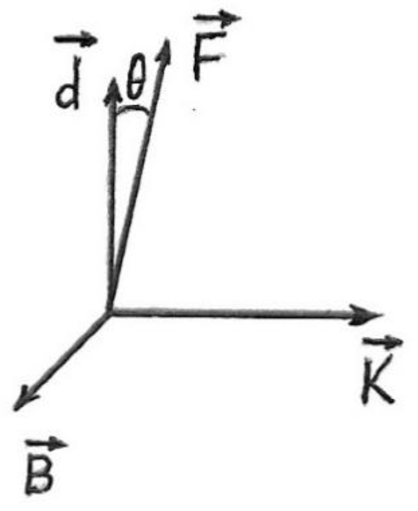
is the scaled detuning from the unperturbed position of the spectral line. Figure 5 presents the orientation of the wave amplitude vector F with respect to the magnetic field B, the pseudomomentum K, and the giant dipole moment d, the latter corresponding to the state within the additional potential well located at x₁ < 0, where x₁ is given by Equation (14).

Under the action of the field Fcosωt, any atomic state possessing a permanent electric dipole moment D manifests in the spectral line profile as a series of Blokhinzew-type satellites at the distances qω (q = ±1, ±2, ±3, …) from the line center (see, e.g., paper [15] and Chapter 3 in book [3]). The actual number of observed satellites depends, first of all, on the so-called modulation parameter

ε = DF/(ħω),

(19)

where DF stands for the scalar product (also known as the dot-product) of these two vectors. If ε << 1, then, at best, practically only the satellites at ±ω might be observed (though not necessarily observed if the spectral line broadening by other mechanisms is relatively large). However, in the case of the GEDM states (the states within the additional potential well) there would be practically always ε >> 1. This situation corresponds to the multi-satellite regime where there would be numerous satellites of significant intensities: The satellites of the maximum intensity would be at Δω ~ ±εω. In this case, even if the spectral line broadening by other mechanisms is relatively large, one could observe the envelope of multiple satellites (rather than individual satellites), the maximum intensity of the envelope being at Δω~±εω. More details and more precise formulas are presented in Chapter 3 of book [3].

Let us denote by g the share of hydrogen atoms that are in the GEDM states (the states within the additional potential well). We consider the case of a relatively weak electrostatic wave in a plasma, so that for hydrogen atoms that are not in the GEDM state, the corresponding modulation parameter from Equation (19) is much smaller than unity. This means that for the share (1 − g) of hydrogen atoms, the would be satellites are extremely weak and practically do not affect spectral line profiles (e.g., for ε~10⁻³, the relative intensity of the “strongest” satellites would be ~10⁻⁶). Then, the total spectral line profile can be represented in the form

S(w) = (1 − g) S₀(w) + gS₁(w),

(20)

where

S₁(w) = Σ J_p²(ε₁) S₀(w − p), ε₁ = e|x₀|(F cosθ)/(ħω),

(21)

In Equation (21), J_p(ε₁) is the Bessel functions and e is the electron charge. As for the function S₀(w) in Equations (20) and (21), it is the shape of the spectral line that would be at the absence of the electrostatic wave. It combines in the standard way the Doppler broadening and the Stark broadening by plasma ions and electrons, as well as the Zeeman effect (see, e.g., books [4,10]).

Below, as an example, we consider the situation where the electrostatic wave in a plasma is the upper hybrid wave propagating perpendicularly to the magnetic field B. Its well-known frequency is (see, e.g., book [17]):

ω = (ω_ce² + ω_pe²)^1/2.

(22)

Here

ω_ce = eB/(m_ec) = 1.76 × 10¹¹B(Tesla),

(23)

is the electron cyclotron frequency (c being the speed of light) and

ωpe = (4πe²N_e/m_e)^1/2 = 5.64 × 10⁴[N_e(cm⁻³)]^1/2

(24)

is the plasma electron frequency, where N_e is the electron density.

For simplicity of formulas, we consider the situation where ω_ce >> ω_pe, which is the case if

B >> B_cr(Tesla) = 3.21 × 10^–7 [N_e(cm⁻³)]^1/2.

(25)

In this case, the upper hybrid wave frequency ω reduces practically to the electron cyclotron frequency ω_ce.

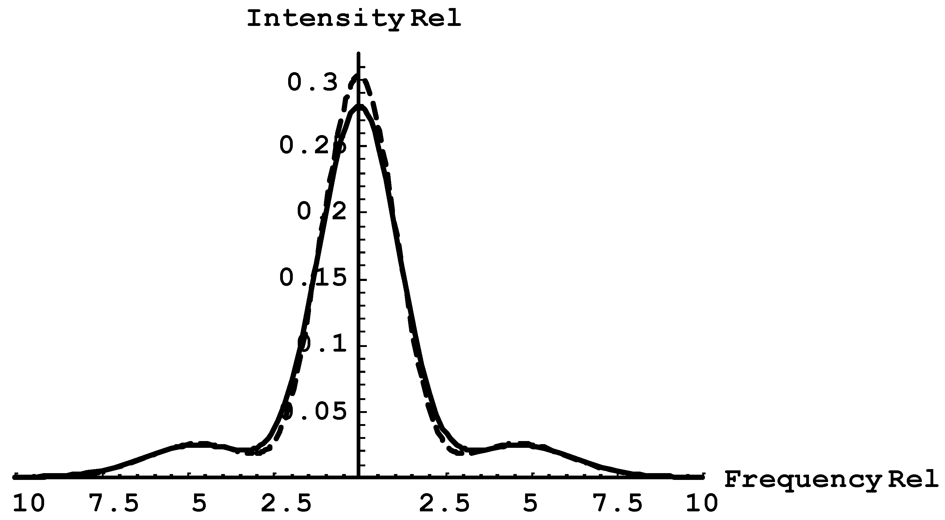
As an example, Figure 6 shows the total profiles S(Δω/ω) of the Ly-beta line (solid curve) and the Ly-alpha line (dashed curve) for the case where g = 0.25, the magnetic field B = 5 Tesla, the plasma temperature T = 3 eV, the electron density N_e = 3 × 10¹³ cm⁻³, the pseudomomentum K = 2.5 × 10⁻¹⁹ g cm/s = 1.25 at. units, and the projection of the amplitude vector of the upper hybrid wave on the giant dipole moment is F cosθ = 10 V/cm. In this case, |x₀| = 3.0 × 10⁻⁴ cm = 5.7 × 10⁴ at. units and ε = 6. We note that B = 5 Tesla, T = 3 eV, and N_e = 3 × 10¹³ cm⁻³ can correspond to the conditions of edge plasmas of tokamaks. The profiles S(Δω/ω) are area-normalized to unity.

It is seen that the quasi-satellites, i.e., the maxima of the envelope of multiple satellites, are located at the same distance (in the frequency scale) from the line center for both spectral lines, this distance being significantly greater than the wave frequency.

Actually, this is true for any two hydrogen lines. This is the distinctive feature of the situation where a share of hydrogen atoms is in the GEDM states. Indeed, if there were not such states and the wave amplitude were large enough for having significant intensities of multiple Blokhinzew-type satellites, the maxima of the satellite envelopes would be at different distances from the line center for different hydrogen lines (see, e.g., book [3], Chapter 3).

In other words, if one would observe quasi-satellites (at the distance from the line center Δω >> ω) in the experimental profile of just one hydrogen line, then both of the above interpretations would be possible. However, if one would observe the quasi-satellites at the same distance from the line center Δω >> ω in the experimental profiles of any two hydrogen lines, then the only possible interpretation would be as follows. First, it would be the manifestation of the presence of the GEDM states of hydrogen atoms. Second, this would constitute a supersensitive method for spectroscopic diagnostics of electrostatic waves in magnetized plasmas, namely, the waves of the amplitude as low as ~10 V/cm or even lower.

4. Discussion

We considered how the GEDM states manifest in the profiles of hydrogen spectral lines in the presence of a quasimonochromatic electrostatic wave of a frequency ω in a plasma. We demonstrated that, in this situation, hydrogen spectral lines can exhibit quasi-satellites, which are the envelopes of Blochinzew-type satellites.

We showed that the distinctive feature of such quasi-satellites is that their peak intensity is located at the same distance from the line center (in the frequency scale) for all hydrogen spectral lines, the distance being significantly greater than the wave frequency ω. At the absence of the GEDM (and for relatively strong electrostatic waves), the maxima of the satellite envelopes would be at different distances from the line center for different hydrogen lines.

We demonstrated that this effect would constitute a supersensitive diagnostic method. It would allow measuring the amplitude of electrostatic waves in plasmas down to ~10 V/cm or even lower. The observation of satellites of two spectral lines in a series should be feasible since the satellites were observed by various experimental groups at different plasma sources for a variety of the electron densities and temperatures (see, e.g., books [3,10,11] where the corresponding experiments were covered).

Finally, we note that this method would not work for diagnosing stochastic quasi-monochromatic waves in plasmas. This is because the maximum of the intensity of the envelope of the satellites, caused by such waves, is at the unperturbed wavelength of the spectral line (rather than being shifted to the wings) (see, e.g., paper [18] and Section 3.2.1 of the book [3]).