On the Temperature and Plasma Distribution of an Inductively Driven Xe-I₂-Discharge

Abstract

Inductively Coupled Plasma (ICP) discharges are part of intense research. Predicting different plasma parameters, like the distribution and temperature of the present species, is of great interest for many applications. Iodine- or halide-containing plasmas in particular have an important function, for example, in the development of mercury-free UV radiation sources. Therefore, a 2D simulation model of a xenon- and iodine-containing ICP was created by using the Finite Element Method (FEM) software COMSOL Multiphysics^®. The included species and the used reactions are presented in this paper. To verify the simulation in relation to the plasma distribution, the results were compared with measurements from literature. The temperature of the lamp vessel was measured in relation to the temperature distribution and also compared with the results of the simulation. It could be shown that the simulation reproduces the plasma distribution with a maximal deviation of ≈6.5% to the measured values and that the temperature distribution in the examined area can be predicted with deviations of up to ≈24% for long vessel dimensions and ≈3% for shorter dimensions. However, despite the deviating absolute values, the general plasma behaviour is reproduced by the simulation. The simulation thus offers a fast and cost-effective method to estimate an effective geometrical range of iodine-containing ICPs.

1. Introduction

In addition to use in plasma thrusters, a main application for iodine- or halide-containing plasmas are mercury-free radiation sources [1,2]. Besides the generation of radiation by using barrier discharges, ICPs for radiation generation were also investigated [3,4]. Because of certain properties, such as the vapour pressure, halide compounds in particular are suitable as a substitute for mercury [5]. Radiation sources containing halides are, therefore, still part of recent research [6]. An electrodeless ICP operation of the lamps provide access to use the full bandwidth of halide compounds as lamp fillings, without the need to consider electrode chemistry as life-limiting process [7].

However, the ignition and operation of inductive mercury-free radiation sources can be difficult [8]. Furthermore, the plasma and temperature distribution have important effects on the discharge. To achieve efficiencies similar to conventional mercury-containing systems, the lamp pressures must be in a comparable range [9]. The lamp pressure is directly dependent on the temperature of the coldest point of the lamp vessel. As the temperature distribution is related to the plasma distribution, this correlation will be considered in the following.

A direct comparison of a pure Xe discharge with a discharge containing a Xe-I${}_2$-mixture shows a difference in the plasma distribution even from the optical appearance. Therefore, a simulation model was developed to investigate this behaviour in more detail. For the simulation, the Finite Element Method (FEM) software COMSOL^® was used [10]. This software includes a module for ICP simulations. The simulation results were compared with the work of Barnes et al. [11] in relation to the plasma distribution. Furthermore, the results of the temperature distribution for the glass vessel were also compared with measurements on a lab system. The simulation model presented in the following shows a useful approximation of the plasma behaviour for future research.

2. Materials and Methods

The plasma model is represented by highly nonlinear coupled systems of differential equations. In order to approximate the plasma behaviour, it is possible to consider the system as a fluid model. This approach will be described more in detail below, as the used software applies the fluid model for simulation [12]. In the fluid model, the plasma is described as a fluid by averaged macroscopic quantities such as density, velocity and energy of the included species. The solution for the macroscopic quantities results from the continuity, momentum, and energy conservation equations. The result are the moment equations of the Boltzmann transport equation [13]. The Boltzmann transport equation assigns a distribution function $f_b=f_b(r,t,\nu )$ of the respective particle density to each species. This depends on the location r, the time t, as well as the velocity $\nu$ and is also dependent to the source or impact term $S\left(f_b\right)$. Thus, the transport equation is given by

$$\begin{array}{c}\hfill \frac{\partial f_b}{\partial t}+\nu ·\overrightarrow{\nabla }{f}_b+\frac{F}{m}·\frac{\partial f_b}{\partial \nu }=S\left(f_b\right)\end{array}$$

(1)

Here, m corresponds to the particle mass and F to the external force acting on the particles, for example, through electromagnetic fields. If the equation is now integrated over the velocity space, the continuity equation already mentioned results in

$$\begin{array}{c}\hfill \frac{\partial n}{\partial t}+\overrightarrow{\nabla }·\overrightarrow{\mathsf{\Gamma }}=S\end{array}$$

(2)

The number of changes due to collisions (e.g., ionization, recombination, etc.) as a function of time and place is given here by S and $\overrightarrow{\mathsf{\Gamma }}$ describes the particle flux. This can be given with help of the drift-diffusion approximation:

$$\begin{array}{c}\hfill \overrightarrow{\mathsf{\Gamma }}=-n\left(\mu \overrightarrow{E}\right)-D\overrightarrow{\nabla }n\end{array}$$

(3)

To determine the energy conservation equation, the transport equation is multiplied by $\frac{1}{2}m{\nu }^2$ and integrated over the velocity space. For the use of the energy, this leads to

$$\begin{array}{c}\hfill \frac{\partial n_{ϵ}}{\partial t}+\overrightarrow{\nabla }·\overrightarrow{{\mathsf{\Gamma }}_{ϵ}}=S_{ϵ}\end{array}$$

(4)

Analogous to the particle flux, the electron energy flux ${\overrightarrow{\mathsf{\Gamma }}}_{ϵ}$ can be calculated:

$$\begin{array}{c}\hfill {\overrightarrow{\mathsf{\Gamma }}}_{ϵ}=-n_{ϵ}\left({\mu }_{ϵ}\overrightarrow{E}\right)-D_{ϵ}\overrightarrow{\nabla }{n}_{ϵ}\end{array}$$

(5)

where all quantities are related to energy. Consequently, $n_{ϵ}$ is the electron energy density, ${\mu }_{ϵ}$ is the electron energy mobility and $D_{ϵ}$ is the corresponding diffusion coefficient of the electron energy. In the software, the quantities are related to the mean electron energy $\overline{ϵ}$ as follows [12]:

$$\begin{array}{cc}\hfill D_{ϵ}=& {\mu }_{ϵ}{T}_e\hfill \end{array}$$

(6)

$$\begin{array}{cc}\hfill {\mu }_{ϵ}=& \frac{5}{3}{\mu }_e\hfill \end{array}$$

(7)

$$\begin{array}{cc}\hfill n_{ϵ}=& n_e\overline{ϵ}\hfill \end{array}$$

(8)

$$\begin{array}{cc}\hfill T_e=& \frac{2}{3}\overline{ϵ}\hfill \end{array}$$

(9)

Here, $T_e$ describes the electron temperature and ${\mu }_e$ the mobility of the electrons. As part of the electron transport calculation, Equation (2) is calculated by the software as follows:

$$\begin{array}{c}\hfill \frac{\partial n}{\partial t}+\overrightarrow{\nabla }·{\overrightarrow{\mathsf{\Gamma }}}_e=R_e-\left(\overrightarrow{u}·\overrightarrow{\nabla }\right)n_e\end{array}$$

(10)

with the vector of fluid velocity $\overrightarrow{u}$, and the electron flux:

$$\begin{array}{c}\hfill {\overrightarrow{\mathsf{\Gamma }}}_e=-n_e\left({\mu }_e\overrightarrow{E}\right)-D_e\overrightarrow{\nabla }{n}_e\end{array}$$

(11)

The source term of the electrons $R_e$ is obtained for all reactions j from the sum of their rate coefficients $k_j$, their mass fraction $x_j$, as well as the neutral particle density $n_n$ and the electron density $n_e$:

$$\begin{array}{c}\hfill R_e=\sum _{j=1}^M{x}_j{k}_j{n}_n{n}_e\end{array}$$

(12)

For this purpose, the rate coefficients can be calculated from the energy-dependent impact cross sections $\sigma \left(ϵ\right)$. COMSOL Multyphysics^® uses the approach:

$$\begin{array}{c}\hfill k_j=\sqrt{\frac{2q}{m_e}}{\int }_0^{\infty }\sigma \left(ϵ\right)ϵf\left(ϵ\right)dϵ\end{array}$$

(13)

The energy-dependent impact cross sections $\sigma \left(ϵ\right)$ are available for many materials and reactions in various databases. The correspondence of the energy conservation Equation (4) for the electron energy density is given in the software as

$$\begin{array}{c}\hfill \frac{\partial n_{ϵ}}{\partial t}+\overrightarrow{\nabla }·\overrightarrow{{\mathsf{\Gamma }}_{ϵ}}=S_{ϵn}-\left(\overrightarrow{u}·\overrightarrow{\nabla }\right)n_{ϵ}+\frac{\left(Q+Q_{gen}\right)}{q}\end{array}$$

(14)

Here, Q and $Q_{gen}$ correspond to the energy input from an external and a general heat source. $S_{ϵn}$ describes the energy gain or loss due to inelastic collisions. $S_{ϵn}$ is formed by the sum of the energy loss $\Delta {ϵ}_j$ due to collisions occurring over all reactions j:

$$\begin{array}{c}\hfill S_{ϵn}=\sum _{j=1}^P{x}_j{k}_j{n}_n{n}_e\Delta {ϵ}_j\end{array}$$

(15)

It is obvious that the rate coefficients $k_j$ and thus the energy-dependent impact cross sections $\sigma \left(ϵ\right)$ play a decisive role in the simulation of the system. Even in a pure Xe-plasma, several hundreds to thousand reactions already take place, some simplifications have to be made. To limit the complexity of the model and still achieve a good approximation of the plasma behaviour, the modeling was initially limited to the most essential reactions. The reactions used are listed in

Table 1. Overview of the reactions and data sources used for the simulation.

Xenon Collision Reactions
No.	Process		Reaction		$\mathsf{\Delta }\mathbf{\epsilon }\left[\mathbf{eV}\right]$	Source
1	Elastic	$\mathrm{Xe}+e$	⟶	$\mathrm{Xe}+e$		[14]
2	Excitation	$\mathrm{Xe}+e$	⟶	$\mathrm{Xe}\left(6s_2\right)+e$	8.31	[15]
3	Excitation	$\mathrm{Xe}+e$	⟶	$\mathrm{Xe}\left(6s_1\right)+e$	8.43	[16]
4	Ionisation	$\mathrm{Xe}+e$	⟶	${\mathrm{Xe}}^{+}+2e$	12.12	[17]
5	Stepwise ionisation	$\mathrm{Xe}\left(6s_2\right)+e$	⟶	${\mathrm{Xe}}^{+}+2e$	3.44	[18]
Xenon Relaxation and Surface Reactions
No.	Process		Reaction		$\mathsf{\Delta }\mathbf{\epsilon }\left[\mathbf{eV}\right]$	Source
6	Relaxation ${}^1$	$\mathrm{Xe}\left(6s_1\right)$	⟶	$\mathrm{Xe}+h\nu$	−8.43	[19]
7	Recombination	${\mathrm{Xe}}^{+}$	⟶	$\mathrm{Xe}$
8	Relaxation	$\mathrm{Xe}\left(6s_1\right)$	⟶	$\mathrm{Xe}$
9	Relaxation	$\mathrm{Xe}\left(6s_2\right)$	⟶	$\mathrm{Xe}$
Iodine Collision Reactions
No.	Process		Reaction		$\mathsf{\Delta }\mathbf{\epsilon }\left[\mathbf{eV}\right]$	Source
10	Dissociative attachment	${\mathrm{I}}_2+e$	⟶	${\mathrm{I}}^{-}+\mathrm{I}$		[20]
11	Elastic	$\mathrm{I}+e$	⟶	$\mathrm{I}+e$		[21]
12	Ionisation	$\mathrm{I}+e$	⟶	${\mathrm{I}}^{+}+2e$	10.45	[22]
Iodine Surface Reactions
No.	Process		Reaction		$\mathsf{\Delta }\mathbf{\epsilon }\left[\mathbf{eV}\right]$	Source
13	Recombination	${\mathrm{I}}^{+}$	⟶	I
14	Decay	${\mathrm{I}}^{-}$	⟶	I
15	Recombination	$\mathrm{I}+\mathrm{I}$	⟶	${\mathrm{I}}_2$

¹ For this reaction the reaction rate of k_j = 2.73 · 10⁸ s⁻¹ was used.

. The reactions are linked in Table 1 with their data sources [14,15,16,17,18,19,20,21,22]. It has to be noted that for a more compact nomenclature of the excited states of Xe the notation of Sommerer [23] was used.

With the used software it was not possible to include the evaporation of the halide in this simulation. For this reason, it was assumed that the material already is completely in the gas phase at the time of ignition. For this purpose, the I${}_2$-vapor pressure curve [24] as well as the lamp volume and the I${}_2$-filling quantity were used to determine the temperature at complete evaporation. The underlying geometries and filling parameters here are listed in

Table 2. Lamp and coil geometry for the I${}_2$ simulation.

Lamp Geometry	Unit	Value	Coil Geometry	Unit	Value
Inner diameter	[mm]	54	Inner diameter	[mm]	59
Outer diameter	[mm]	56	Outer diameter	[mm]	67
Length	[mm]	78	Length	[mm]	75
Volume	[cm${}^3$]	111	Frequency	[MHz]	3
Filling pressure	[Pa]	100	Windings		8
Starting gas		Xe
Filling material		I${}_2$
Amount of solid	[mg]	1.0
Calculated initial pressure	[Pa]	190

. Subsequently, the pressure difference $\Delta p$ to the real initial pressure was determined with the temperature and the particle number of the starting gas as well as the I${}_2$-filling quantity according to the ideal gas law. This was used as initial pressure to simulate the discharge. An overview of the pressure curves obtained in this way can be seen in Figure 1.

By means of this procedure, it is now possible to simulate the parameters of the discharge numerically without including the evaporation. The disadvantage of this approach is that the simulation can only be expected to provide reliable approximations of the plasma behaviour from the point at which an unsaturated operation is reached. Nevertheless, the simulation model provides a good estimation of the plasma parameters, as described below.

3. Results and Discussion

The following section is divided into two subsections. In the first subsection, the results are presented and discussed in relation to the plasma distribution. The second subsection describes the effect of the plasma distribution on the temperature distribution on the glass vessel as well as gas temperature distribution in the plasma.

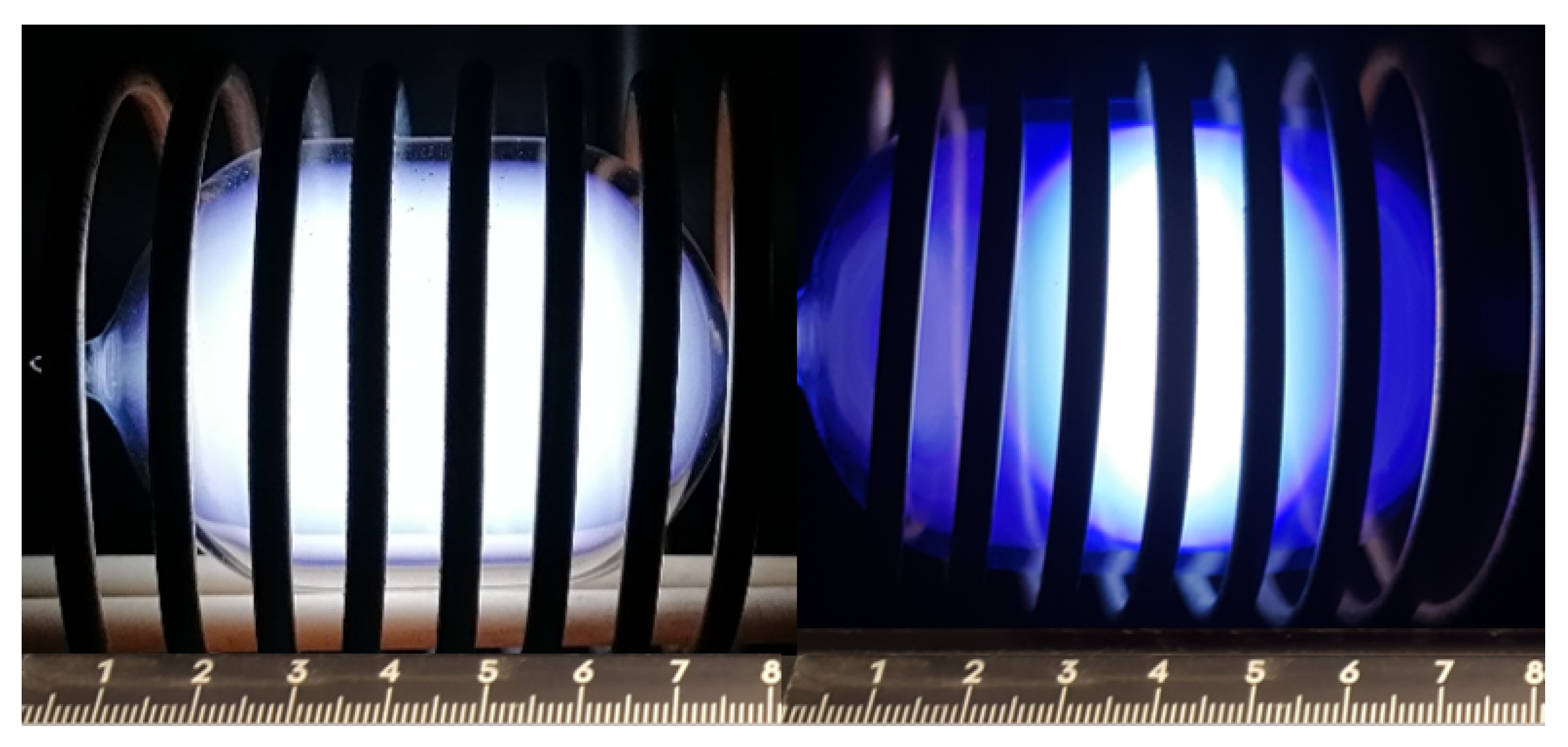
3.1. Plasma Distribution

By directly comparing an I${}_2$-containing Xe discharge to a pure Xe discharge, several differences are noticeable. As shown in Figure 2, the electron density behaves clearly different. For example, the electron density in the Xe discharge at 400 W input power reaches a mean value of $n_e=6.8·{10}^{14}$ cm${}^{-3}$. The I${}_2$-containing discharge has a lower mean electron density with only $n_e=4.8·{10}^{10}$ cm${}^{-3}$.

This significant deviation at the same input power, geometry, and pressure can be justified by reaction 10 in Table 1. This reaction is due to the high electronegativity of iodine and the resulting possibility of dissociative attachment of electrons to form anions. Through this process, the electron density is significantly reduced compared to the pure Xe plasma. In the shown case, the mean electron density is reduced by approximately 4 orders of magnitude. A shift in the electron density distribution in contrast to the pure Xe discharge is also clear in Figure 2. This can be explained by the previously mentioned process too. The different behaviour becomes particularly clear by comparing the electron density distribution with the I${}^{-}$- and the I-distribution. Figure 3 shows the mentioned distributions.

The I${}^{-}$ distribution shows the increase in particle density on the edge regions. If the radial I${}_2$ distribution is considered, the highest concentration is also reached on the edge regions. This behaviour in I${}_2$-containing inductive discharges is known and based on the recombination of dissociated iodine atoms at the wall [11]. To verify the simulation, a model was created with the geometry and parameters as described by Barnes et al. in [11]. A comparison of the radial I${}_2$-distribution between the simulation carried out and the measurements of is shown in Figure 4.

The irregularly distributed simulated points in Figure 4 are based on the meshing of the model. The figure shows that the simulation approximates the measurements well. To determine the deviation, the measured values were interpolated and the maximum deviation was determined. The maximum deviation results in the curve slope with ≈6.5% to the measured values. A comparison with the simulation results of the geometry and parameters used in this paper is also shown. The results indicate that the general plasma behaviour with an increasing I${}_2$-density at the edges of the lamp vessel can also be assumed here. The described and simulated behaviour has direct effects on the plasma. This is particularly evident in the temperature distribution, which is explained more in detail in the next section.

3.2. Temperature Distribution

In relation to the temperature distribution in the lamp systems, the dimension of the lamp vessels play a decisive role. With a given frequency, power, pressure, and coil, only the geometry remains as a parameter to influence the temperature distribution. In lamps containing halides, the filling components condense at the coldest point of the system. To generate medium to high pressures, the aim is to create a temperature distribution that is as homogeneous as possible. However, this is only partly achievable due to the behaviour of the plasma. It has been observed that in the case of halide-containing discharges, the plasma tends to form a sphere which can already be seen in Figure 5.

Here, the temperature behaviour is already visually observable by the plasma distribution. This behaviour means that the coldest point is always at the ends of the lamp due to the plasma behaviour. As the hottest point is therefore in the middle of the lamp, the coldest point is also determined by the lamp length. Therefore, temperature measurements were carried out at different lamp lengths. A thermographic camera was used to measure the lamp temperature (A325, FLIR Systems, Wilsonville, OR, USA). This method allows to monitor the temperature on the entire surface of the lamp vessel and to identify the hottest and the coldest point on the surface. The values used were measured after thermal stabilization of the lamp. These measurements can be seen in Figure 6. Note that with this method only the temperatures on the outer glass vessel can be recorded.

The measurement shows that the behaviour has a significant influence on the temperature distribution. From the hottest point in the center of the lamp, the temperature drops significantly towards the ends of the lamp. Despite the different lengths, the lamp bodies have a similar temperature distribution. For illustration, the quotient $T_q$ of the measured maximum temperature $T_{max}$ and the minimum temperature $T_{min}$ is compared. $T_q$ results as

$$T_q=\frac{T_{max}}{T_{min}}$$

(16)

In order to achieve a homogeneous temperature distribution on the outer glass vessel, a geometry should be chosen, so that it has the smallest possible value of $T_q$. Since the temperature decreases from the center along the length of the lamp, the shortest lamp length results in the smallest temperature ratio from the hottest to the coldest point. In order to verify the simulation model, the simulated temperature quotient was compared to the measured one. The results are shown in Figure 7.

The comparison shows a large deviation of the simulation from the measurement at longer lamp lengths with a maximal deviation of ≈24%. For smaller lamp lengths, deviations of ≈3% are achieved. From the simulation and the measurement, it can be seen that the temperature quotient $T_q$ approaches a homogeneous distribution for shorter lamp lengths. As shown in Figure 8, the lamp length has only a small influence on the temperature distribution in the plasma.

The simulation shows that even with longer lamp geometries, the plasma is still concentrated in the center of the lamp, this behaviour considers to be consistent with the results in Figure 5. This means that it is not possible to select a lamp geometry of arbitrary length if a homogeneous temperature distribution over the entire glass vessel of the plasma is desired.

4. Conclusions

In this work, a 2D model for the simulation of Xe-I${}_2$ plasmas was presented. The simulation results were compared with other publications in relation to the plasma distribution. The temperature distribution was also simulated and compared with own experimental results. It could be shown that the simulation can reproduce the measurements from the literature in terms of the plasma distribution with a maximum deviation of ≈6.5%. The results suggest that also other plasma parameters such as the plasma impedance, which is influenced by the contained species, could be determined by the simulation with small deviations as well. Therefore, the simulation could be a useful tool for designing appropriate power supplies.

The simulation of the temperature distribution deviates significantly from the measured values for longer geometries. For small lamp lengths, the simulation results match the measurements with a deviation of ≈3%. A precise consideration of the validity limits beyond the areas analyzed needs further investigation. Nevertheless, the results show that the simulation reproduces the general temperature behaviour and could be used to estimate reasonable lamp geometries.

References

1. Grondein, P.; Lafleur, T.; Chabert, P.; Aanesland, A. Global model of an iodine gridded plasma thruster. Phys. Plasmas 2016, 23, 033514. [Google Scholar] [CrossRef]
2. Shchedrin, A.; Kalyuzhnay, A. Numerical Simulation of Plasma Kinetics in Low-Pressure Discharge in Mixtures of Helium and Xenon with Iodine Vapours. Numer. Simul. Phys. Eng. Process. 2011, 257. [Google Scholar] [CrossRef] [Green Version]
3. Avdeev, S.M.; Zvereva, G.N.; Sosnin, E.A.; Tarasenko, V.F. XeI barrier discharge excilamp. Opt. Spectrosc. 2013, 115, 28–36. [Google Scholar] [CrossRef]
4. Shuaibov, A.K.; Grabovaya, I.A.; Gomoki, Z.T.; Kalyuzhnaya, A.G.; Shchedrin, A.I. Output characteristics and parameters of the plasma from a gas-discharge low-pressure ultraviolet source using helium-iodine and xenon-iodine mixtures. Tech. Phys. 2009, 54, 1819–1824. [Google Scholar] [CrossRef]
5. Käning, M.; Hitzschke, L.; Schalk, B.; Berger, M.; Franke, S.; Methling, R. Mercury-free high pressure discharge lamps dominated by molecular radiation. J. Phys. D Appl. Phys. 2011, 44, 224005. [Google Scholar] [CrossRef] [Green Version]
6. Mayor-Smith, I.; Templeton, M.R. Development of a mercury–free ultraviolet high–pressure plasma discharge for disinfection. Water Environ. J. 2021, 35, 41–54. [Google Scholar] [CrossRef] [Green Version]
7. Wharmby, D.O. Electrodeless lamps for lighting: A review. IEE Proc. A Sci. Meas. Technol. 1993, 140, 465. [Google Scholar] [CrossRef]
8. Tim, G.; Qihao, J.; Fabian, D.; Santiago, E.; David, K.; Rainer, K. Reducing the Transition Hysteresis of Inductive Plasmas by a Microwave Ignition Aid. Plasma 2019, 2, 341–347. [Google Scholar] [CrossRef] [Green Version]
9. Phillips, R. Sources and Applications of Utraviolet Radiation; Acad. Pr: London, UK, 1983. [Google Scholar]
10. COMSOL Multiphysics® v. 55; COMSOL AB: Stockholm, Sweden. Available online: www.comsol.com (accessed on 8 November 2021).
11. Barnes, P.N.; Kushner, M.J. Formation of XeI(B) in low pressure inductive radio frequency electric discharges sustained in mixtures of Xe and I 2. J. Appl. Phys. 1996, 80, 5593–5597. [Google Scholar] [CrossRef] [Green Version]
12. COMSOL. Comsol Plasma Module User’s Guide v. 55; COMSOL AB: Stockholm, Sweden, 2020. [Google Scholar]
13. Meiners, A. Entwicklung, Charakterisierung und Anwendungen Nichtthermischer Luft-Plasmajets. Ph.D. Thesis, Georg-August-Universität, Göttingen, Germany, 2011. [Google Scholar]
14. Hayashi Database. Available online: https://us.lxcat.net/cache/618927e7ceed8/ (accessed on 12 November 2020).
15. Biagi-v7.1. Available online: https://us.lxcat.net/cache/618928fdbba3d/ (accessed on 12 November 2020).
16. MAGBOLTZ, S. Biagi.12. Available online: https://us.lxcat.net/cache/618929767de6c/ (accessed on 12 November 2020).
17. TRINITI Database. Available online: https://us.lxcat.net/cache/6189287ab0ca0/ (accessed on 12 November 2020).
18. SIGLO Database. Available online: https://us.lxcat.net/cache/618929f34b485/ (accessed on 12 November 2020).
19. Kramida, A.; Ralchenko, Y. NIST Atomic Spectra Database, NIST Standard Reference Database 78; National Institute of Standards and Technology: Gaithersburg, MD, USA, 1999. [CrossRef]
20. Biondi, M.A.; Fox, R.E. Dissociative Attachment of Electrons in Iodine. III. Discussion. Phys. Rev. 1958, 109, 2012–2014. [Google Scholar] [CrossRef]
21. Zatsarinny, O.; Bartschat, K.; Garcia, G.; Blanco, F.; Hargreaves, L.R.; Jones, D.B.; Murrie, R.; Brunton, J.R.; Brunger, M.J.; Hoshino, M.; et al. Electron-collision cross sections for iodine. Phys. Rev. A 2011, 83, 107. [Google Scholar] [CrossRef] [Green Version]
22. Ali, M.A.; Kim, Y.K. Ionization cross sections by electron impact on halogen atoms, diatomic halogen and hydrogen halide molecules. J. Phys. B At. Mol. Opt. Phys. 2008, 41, 145202. [Google Scholar] [CrossRef]
23. Sommerer, T.J. Model of a weakly ionized, low-pressure xenon dc positive column discharge plasma. J. Phys. D Appl. Phys. 1996, 29, 769–778. [Google Scholar] [CrossRef]
24. Hansen, S.; Getchius, J.; Steward, R.; Brumleve, T. Vapor Pressure of Metal Bromides and Iodides: With Selected Metal Chlorides and Metals, 2nd ed.; APL Engineered Materials, Inc.: Urbana, IL, USA, 2006. [Google Scholar]
Figure 1. Pressure curve over the temperature of a discharge with 100 Pa of Xe as well as 1 mg of I 2 . The green marked area corresponds to the area of an unsaturated discharge.
Plasma 04 00037 g001
Figure 2. Comparison of the electron density distribution at 400 W input power with 3 MHz and an initial pressure of 190 Pa. Left: Xe discharge. Right: I 2 -Xe-discharge.
Plasma 04 00037 g002
Figure 3. Comparison of different particle density distributions of the I 2 -Xe plasma at 400 W input power. Left: Electron density. Center: Atomic iodine density. Right: I -density.
Plasma 04 00037 g003
Figure 4. I 2 -particle density distribution along the lamp radius in the middle of the vessel. Comparison of the measurements of Barnes et al. [11], indicated with n B m ; a simulation using the same parameters and geometry, indicated with n B s ; and the simulation with the geometry and parameters presented in this paper, indicated as n s .
Plasma 04 00037 g004
Figure 5. Comparison of the plasma distribution of pure gas- to halide-filled lamp systems at 400 W input power. Left: Xe-filled lamp system. Right: Xe-I 2 -filled lamp system.
Plasma 04 00037 g005
Figure 6. Measurement of the temperature distributions for different lamp lengths. The zero was set at the hottest point.
Plasma 04 00037 g006
Figure 7. Comparison of the simulation and measurements of the temperature quotient T q .
Plasma 04 00037 g007
Figure 8. Comparison of plasma temperature distribution with different lamp lengths. Here, a coil with 15 windings was simulated to reproduce the real system for the measurement.
Plasma 04 00037 g008