Article

Adaptive Active Disturbance Rejection Control for Vehicle Steer-by-Wire under Communication Time Delays

1
Department of Automated Manufacturing, Al Khwarizmi College of Engineering, University of Baghdad, Baghdad 10071, Iraq
2
School of Science, Computing and Engineering Technology, Swinburne University of Technology, Melbourne 3122, Australia
3
Electrical Engineering College, Shandong University of Aeronautics, Binzhou 256600, China
*
Author to whom correspondence should be addressed.
Appl. Syst. Innov. 2024, 7(2), 22; https://doi.org/10.3390/asi7020022
Submission received: 25 January 2024 / Revised: 21 February 2024 / Accepted: 5 March 2024 / Published: 8 March 2024
(This article belongs to the Section Control and Systems Engineering)

Abstract

:
In this paper, an adaptive active disturbance rejection control is newly designed for precise angular steering position tracking of the uncertain and nonlinear SBW system with time delay communications. The proposed adaptive active disturbance rejection control comprises the following two elements: (1) An adaptive extended state observer and (2) an adaptive state error feedback controller. The adaptive extended state observer with adaptive gains is employed for estimating the unmeasured velocity, acceleration, and compound disturbance which consists of system parameter uncertainties, nonlinearities, exterior disturbances, and time delay in which the observer gains are dynamically adjusted based on the estimation error to enhance estimation performances. Based on the accurate estimations of the adaptive extended state observer, the proposed adaptive full state error feedback controller is equipped with variable gains driven by the tracking error to develop control precision. The integration of the advantages of the adaptive extended state observer and the adaptive full state error feedback controller can improve the dynamic transient and static steady-state effectiveness, respectively. To assess the superior performance of the proposed adaptive active disturbance rejection control, a comparative analysis is conducted between the proposed control scheme and the classical active disturbance rejection control in two different cases. It is worth noting that the active disturbance rejection control serves as a benchmark for evaluating the performance of the proposed control approach. The results from the comparison studies executing two simulated cases validate the superiority of the suggested control, in which estimation, tracking response rate, and steering angle precision are greatly improved by the scheme proposed in this article.

1. Introduction

From approximately 1980s till now, steer-by-wire (SBW) systems have garnered significant attention from researchers in the domain of control application [1]. SBW systems employ electric motors and corresponding driving control systems as an alternative to mechanical linkages [2,3]. To be specific, to improve the stability and dependability of steering vehicles, the shaft connecting the steering wheel and the front wheels is removed [4]. Instead, an electric motor which is denoted as the steering motor is utilized to drive the front wheels. Furthermore, to allow drivers a sense of various tyre self-aligning forces, a feedback motor is mounted near the steering wheel. However, various uncertainties, including parameter variations of the SBW model and external disturbances induced by various road conditions, pose challenges to conventional control algorithms such as proportional-derivative control. These uncertainties prevent the front wheels from accurately following the driver’s intended actions and even make the system unstable. Therefore, the enhancement of the front wheels’ tracking accuracy and robustness against uncertainties emerge as crucial research topics in the SBW systems [5].
To bolster the tracking precision and robustness of various sources of uncertainty, the disturbance/uncertainty estimation and attenuation (DUEA) techniques have been garnering significant attention over the past several decades. It is worth noting that active disturbance rejection control (ADRC), as well as disturbance observer-based control (DOBC), fall under the umbrella of DUEA techniques [6], i.e., an observation methodology is established to estimate the disturbances or uncertainties, with the estimation results then utilized to compensate for uncertainties within a robust controller. In [7], the ADRC is effectively utilized to ensure precise control of the angular position of the front wheels, enabling them to accurately follow the movements of the steering wheel against uncertainties such as the self-aligning torque. To enhance the controller’s robustness even further, sliding mode control (SMC) is seamlessly integrated into the ADRC in [8]. To enhance the convergence rate of the SMC, the fractional-order SMC is introduced in the SBW system to enhance the integral and derivative actions, thereby increasing the parameter optimization space and improving tracking performance [4]. In these references, the extended state observer (ESO) is adopted in ADRC to compensate for uncertainties. Due to the potential presence of extensive unknown nonlinearities and uncertainties in SBW systems, refs. [9,10] considered the application of neural networks (NNs) to enhance the SBW systems’ uncertainty estimation performance. The underlying rationale is that NNs possess the remarkable capability to approach various functions with arbitrary precision under specific conditions. Please notice that the controller gains mentioned in the literature above are constant, i.e., they are fixed values and determined before operating the control algorithms.
Adaptive control belongs to crucial control methodology to deal with time-varying model parameters [2,11]. In addition, it can be seamlessly integrated with various control algorithms in the SBW systems [12,13,14,15,16,17,18,19]. In [12], a prior equation is adopted to estimate and compensate for the self-aligning torque. Moreover, an adaptive law is tailored to determine the gain of this equation. The outcome of the prior equation is delivered to a feedback motor, enabling it to produce a responsive force that replicates the ’road feels’ for the driver. In addition, it serves as a crucial uncertainty compensation in the fast non-singular terminal SMC (FNTSMC). This uncertainty compensation component effectively mitigates the impact of a self-aligning torque. However, as the prior equation may contain noise and uncertainty and it cannot be used to estimate unavailable system states such as angular velocity of the steering motor, an adaptive sliding mode observer (ASMO) as well as a Kalman filter (KF) are employed in [15] to improve estimation performance of SBW system states. To further improve the estimation rate, an adaptive fixed-time state observer (AFTSO) is proposed to compute the front wheels’ speed in [17]. An adaptive SMC (ATSMC) terminal is proposed in [19]. In this work, the bounds of the system parametric uncertainty and the external disturbances are compensated by the adaptive laws in the reaching law of ATSMC. Given that disturbances in SBW systems can be categorized as a predictable part and a bounded unknown component, ref. [14] utilizes the Luenberger observer to estimate the former. In [13], the adaptive law is applied to determine the output layer parameters of the extreme learning machine (ELM) which is designed to compensate for the lumped uncertainty. As the precise bounds on some state-dependent uncertainties of the SBW systems may not be known, ref. [18] suggests the implementation of an adaptive control approach that eliminates the need for prior knowledge of uncertainty structures and bounds. Unfortunately, the aforementioned references fail to consider the negative impact of communication time delays in SBW systems, which may hinder the practical implementation of these methods.
In terms of SBW systems, the control input is voltage which is utilized to regulate the steering motor, while the angular position of the front wheels serves as the feedback [12]. However, the introduction of the CAN bus in these systems introduces communication time delays in both the control input (denoted as input delay) and the feedback signal (denoted as output delay) [20,21]. Since the input and output delays can considerably affect control performance [22,23], it is imperative to consider them during the controller design process. Thus, ref. [21] introduces a layered time-delay robust control strategy (LTDRCS) to address large random time delays in SBW systems. Nevertheless, this strategy does not account for uncertainty estimation and compensation, and the selection of control parameters can be complex. In another recent study [24], the time-delayed knowledge of control input and system states is utilized to compute uncertainties. However, this approach necessitates precise knowledge of the past values of control input and system states, thereby posing practical implementation challenges.
The human–machine interface (HMI) has found widespread applications in many automated systems, including those pertaining to SBW systems [25]. However, in highly automated systems, the design of the HMI is primarily influenced by technological advancements, rather than the expertise of the individuals who drive the vehicles. In practice, drivers may not fully comprehend the operations performed through the HMI [26]. In scenarios such as the emergence of traffic conditions, the safety of drivers is compromised. As a potential solution, it is imperative to develop HMIs for the SBW systems that offer intuitive and user-friendly information specifically tailored for drivers to enhance driving experience, usability, and safety. Another practical challenge for the SBW system lies in its fault-tolerant capability. Specifically, all components of the steering system should possess fault-tolerant features to accommodate at least one failure [27]. One potential solution to this challenge is to employ multiple identical units operating in parallel. In the event of a failure in one unit, the backup units can seamlessly take over, ensuring continued operation. However, this solution comes with added costs and results in an increase in system volume. An alternative approach to enhancing reliability without adding weight or cost to the system is to utilize estimation techniques, including the implementation of state observers [27].
In this paper, motivated by the published work of time-varying ADRC design in [28], a novel time-varying adaptive gain ADRC is proposed for the uncertain nonlinear SBW plant under communication time delays. The proposed AADRC has two components: the adaptive ESO (AESO) and adaptive full-state error feedback control (AFSEFBC). The main contributions are summed up as follows:
  • Large time delays in a communication channel that the second-order SBW suffers are considered, therein a first-order Taylor series expansion is introduced to address the time delays. However, the order of SBW becomes three; thus, the increase in system order makes the control tasks more complicated. To solve the complexity arising from the Taylor approximation, we propose a novel active disturbance rejection control (AADRC) for the time-delayed SBW subject to system uncertainties and disturbances from external factors.
  • Because of consideration and approximation of the time delays, the overall disturbances acting on the SBW become very large. To overcome this issue, we lump the nonlinearities, uncertainties, and external disturbances of the SBW that are separated from the total disturbances. Such separation of disturbances makes the feasibility of application of the novel AADRC which is a combination of AESO and AFSEFBC.
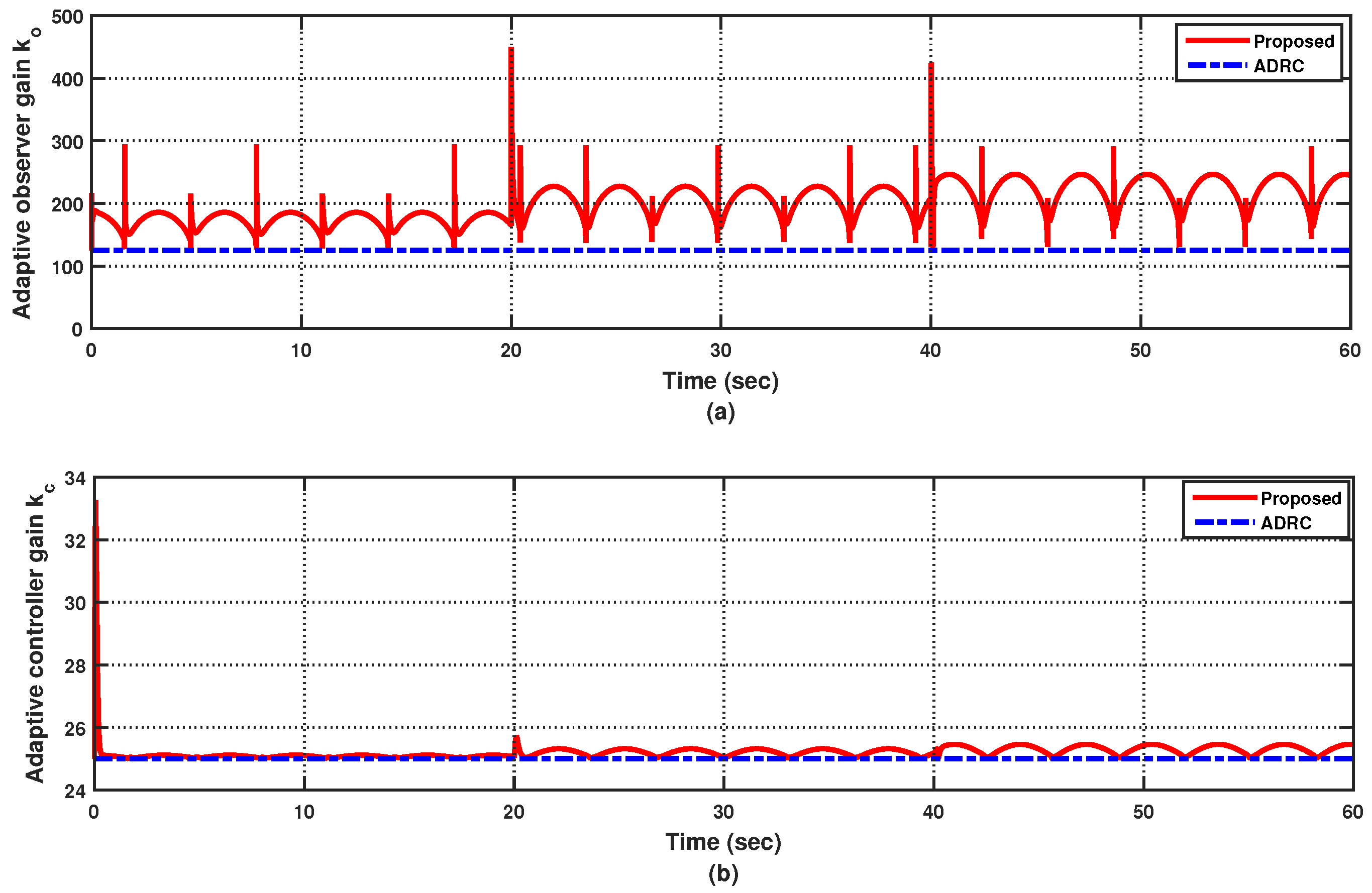
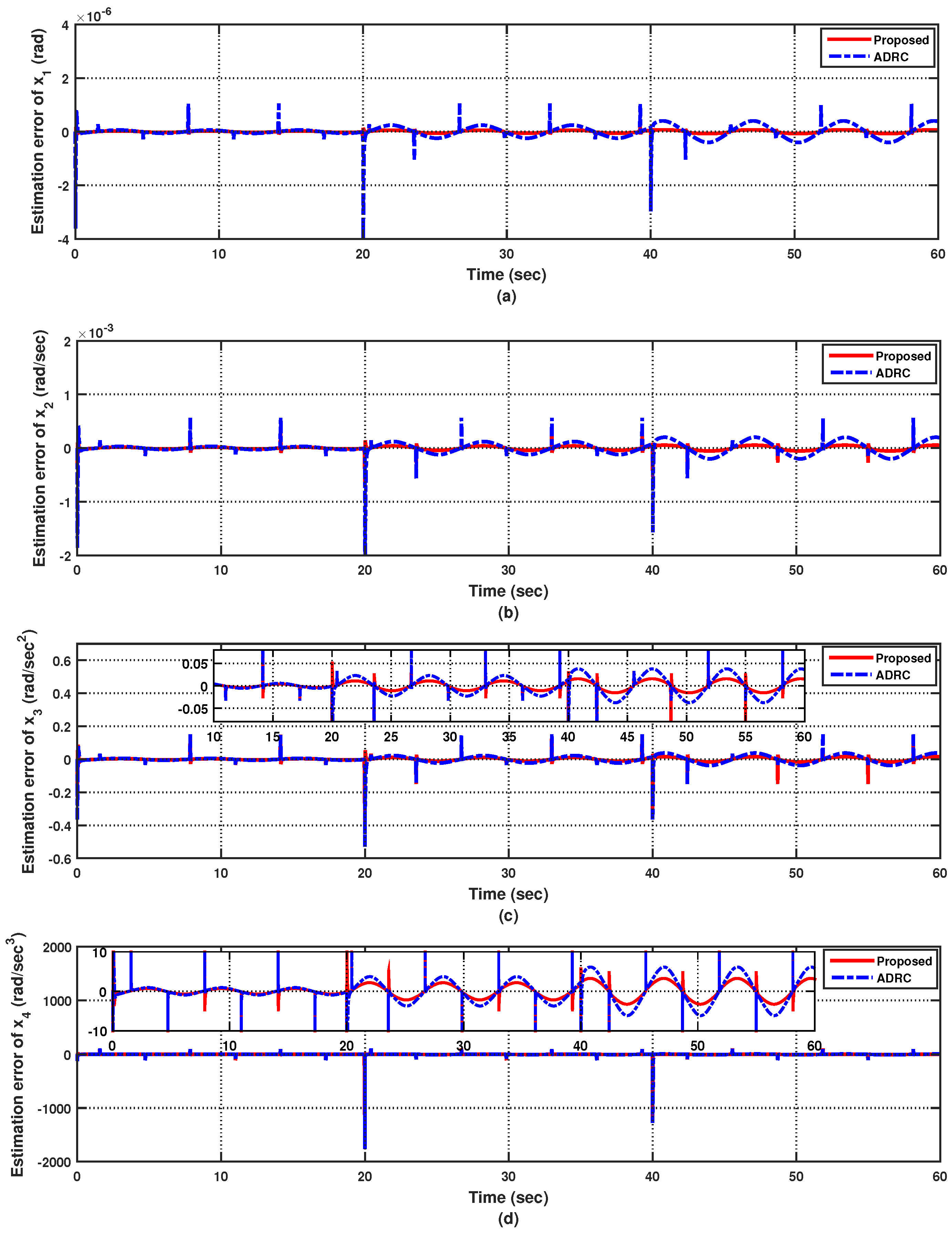
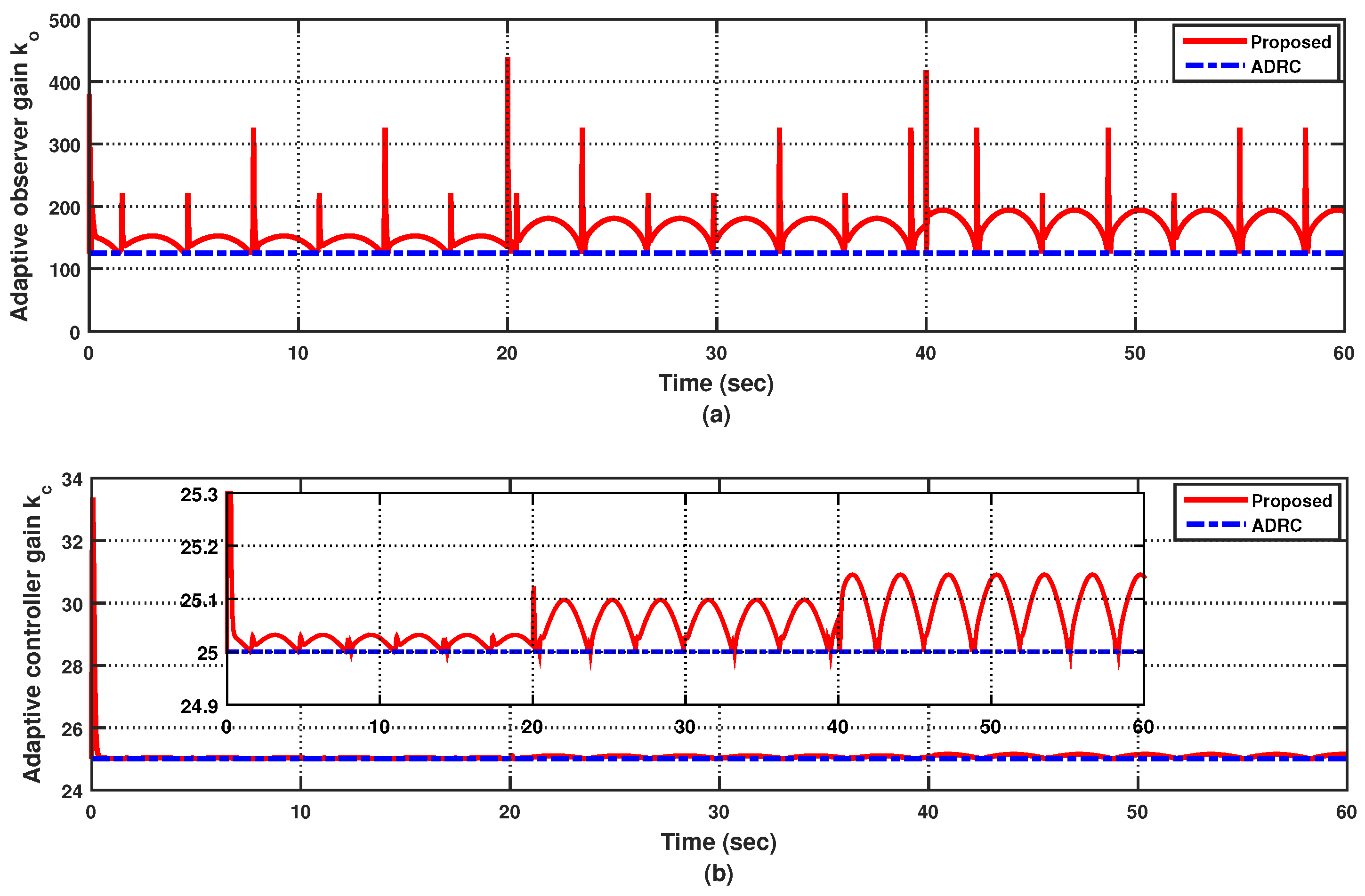
  • A novel AESO is proposed to estimate unmeasured velocity and acceleration, as well as the lumped disturbance with better estimation precision, low computation cost, and minimum peak phenomenon. Adaptive gains of the AESO are updated online based on a position estimation error to improve estimation performance.
  • A novel AFSEFBC is improved to enhance the trajectory tracking efficiency of the angular steering position of the front wheel, in which its gains are adjusted online according to the position tracking error, and thus the angular steering position is improved in terms of lesser overshoot and better steady state.
  • The boundedness of the estimation and the tracking error of the closed-loop stability of the AESO and AFSEFBC, respectively, is rigorously analyzed.
Finally, two simulation cases with a comparison with the standard ADRC are carried out to show the validity of the suggested AADRC scheme.
The remainder of this text is structured as follows: Section 2 introduces the SBW plant represented by the benchmark simulation model. Section 3 presents the novel adaptive ADRC design procedure for the time-delayed SBW system, which is divided into subsections of designing AESO and AFSEFBC. In this section, the boundedness of estimation and tracking errors of the AESO and AFSEFBC, respectively, are analyzed. Then, in Section 4, the efficiency and feasibility of the proposed control scheme are validated by simulation results from the simulative SBW vehicle. Finally, Section 5 describes the conclusions of this full text with future work.

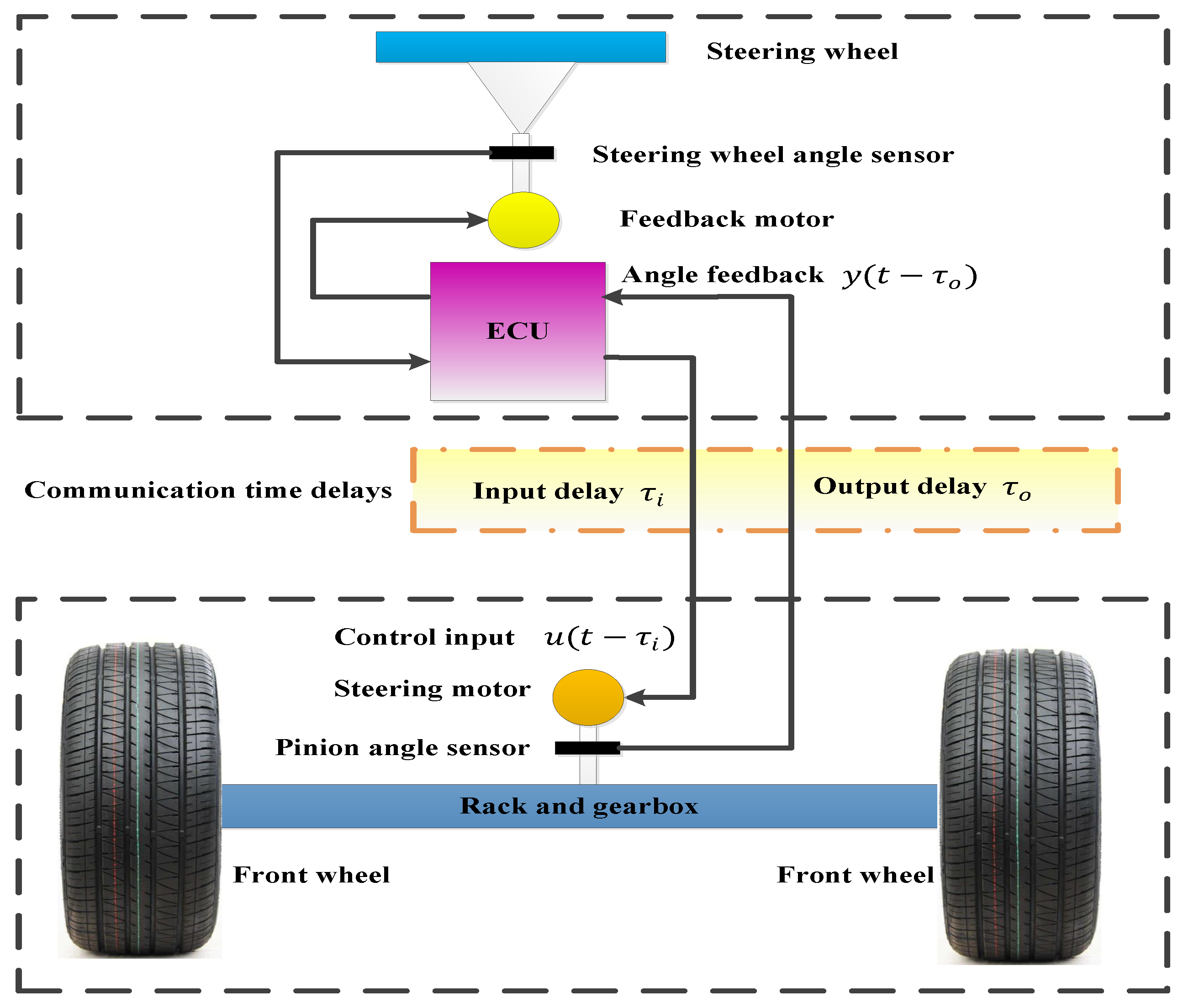
2. SBW Plant Dynamical Modeling

2.1. Structure of the SBW Plant

Figure 1 illustrates the schematic system of the SBW. It is composed of three main parts: the middle part contains the communication time delays, the upper part is the hand/steering wheel that interfaces with the drivers, and the lower part is the steering actuator module that produces the vehicle’s steering responses. A steering motor takes the place of the mechanical link between the steering wheel and the steering actuation, as opposed to traditional hydraulic or electrical power steering systems. The driving command for the steering motor and the angular feedback are both transmitted through signal wires in the SBW system’s operating principle. The key concern for the SBW system is high-precision tracking control of the front wheels to follow its corresponding reference of the steering wheel provided by drivers to ensure precise steering efficiency.

2.2. Dynamical Modeling of the Nominal SBW Plant with Uncertainties

The differential equation of motion for the SBW plant can be expressed as follows using the simplified model of the SBW system described in [29]:
J e θ ¨ s + B e θ ˙ s = κ u τ c τ sel κ = κ 1 · κ 2 · κ 3 · κ 4 τ c = ξ f sign ( θ ˙ s )
where θ s , θ ˙ s , and θ ¨ s , are, respectively, the angular position, velocity, and acceleration of the steering motion of the front wheels; u indicates the steering motor unit’s voltage torque that is designed by the proposed controller; τ s e l is the self-aligning torque applied to the steering system; τ c is the frictional torque caused by the Coulomb friction; and sign ( · ) is the standard signum function. Table 1 lists all of the other system parameters and their corresponding descriptions, values, and units. Additionally, Table 1 provides the scaling factors related to κ along with their respective descriptions and values.
It should be noted that, for the purposes of this study, κ can be regarded as a constant because, at least for the duration of our investigation, its value does not change noticeably over time. Nonetheless, the nonlinearities and external disturbances of the model may lead to unpredictable and fluctuating system parameters [2]. The system temperature fluctuations, erratic external road loads that result in tiny deformations in the steering system, and other factors can all contribute to these parameter variations. The parametric uncertainties can be regarded as bounds, according to [2], and are given here with corresponding bounds.
| Δ J e | = | J e J e 0 | Δ ¯ J e ; ( Δ ¯ J e = 0.1 J e 0 ) | Δ B e | = | B e B e 0 | Δ ¯ B e ; ( Δ ¯ B e = 0.1 B e 0 ) | Δ ξ f | = | ξ f ξ f 0 | Δ ¯ ξ f ; ( Δ ¯ ξ f = 0.1 ξ f 0 )
where J e 0 , B e 0 , and ξ f 0 represent the nominal components of the SBW model parameters; Δ J e , Δ B e , and Δ ξ f denote the uncertain parts of the SBW model parameters; Δ ¯ J e , Δ ¯ B e , and Δ ¯ ξ f refer to the upper bounds of the corresponding model parameters.
The velocities of the front wheels cannot always be measured due to practical constraints of the SBW system. Moreover, a front-wheel camber angle that is too inadequate may arise from the absence of weight distribution on the front wheels [30]. Consequently, during the steering process, the tires might not sense exact self-aligning torques. In our investigation, we assume that the tire slip angles are small. Therefore, to approximate the self-aligning torque, a hyperbolic tangent function can be used [31,32] as
τ sel = ρ τ tan h ( θ s )
where ρ τ is the time-varying coefficient related to various road statuses; it is given elaborately in Simulation Outcomes section. In addition, we define function tan h ( · ) as in the following expression:
tan h ( z ) = e 2 z 1 e 2 z + 1 .
Regarding the model uncertainties in (2) with external disturbances d ( t ) that the SBW plant dynamic is subject to, the differential motion equation of this SBW plant in (1) can be expressed as
( J e 0 + Δ J e ) θ ¨ s + ( B e 0 + Δ B e ) θ ˙ s = κ u ( ξ f 0 + Δ ξ f ) sign ( θ ˙ s ) τ sel + d ( t )
which can be concisely rearranged to have
θ ¨ s = B e 0 J e 0 θ ˙ s + κ J e 0 u + D ( θ s , t )
where
D ( θ s , t ) = 1 J e 0 [ ξ f 0 sign ( θ ˙ s ) Δ J e θ ¨ s Δ B e θ ˙ s Δ ξ f sign ( θ ˙ s ) τ sel + d ( t ) ]
and D ( x , t ) R represents the lumped disturbance, including model uncertainties, external disturbances, etc.
We define x 1 = θ s and x 2 = θ ˙ s to be the SBW system states; thus, the state space form of the nonlinear second-order perturbed systems SBW modeled in (6) is as follows:
x ˙ 1 = x 2 x ˙ 2 = F 0 ( t , x ) + b 0 u + + D ( x , t ) y = x 1
with
F 0 ( x , t ) = B e 0 J e 0 θ ˙ s = a 20 θ ˙ s ; and b 0 = κ J e 0
where vector x = [ x 1 , x 2 ] T R 2 represents the system states, y R stands for the output of the SBW plant, u R is the AADRC input to be designed, and F 0 ( x , t ) R is the nominal dynamic of the SBW system.

2.3. Dynamical Modeling of the Time-Delayed SBW Plant with Uncertainties

The connection between the steering wheel located in the upper section and the steering motor located in the lower section is made through the transmission channel, as seen in Figure 1. Time delays of τ i for the input and τ o for the output are introduced by this connection. The uncertain SBW system presented in (7) can be reformulated as follows by accounting for the time delays in the transmission channel:
x ˙ 1 ( t ) = x 2 ( t ) x ˙ 2 ( t ) = F 0 ( t , x ) + b 0 u ( t τ i ) + D ( x , t ) y = x 1 ( t τ o ) .
As stated in [33], the overall delay, τ , is determined by summing the input delay, τ i , and the output delay, τ o , which is the time-varying parameter. At this point, the SBW system’s dynamical modeling in (8) is rethought by
x ˙ 1 ( t ) = x 2 ( t ) x ˙ 2 ( t ) = F 0 ( t , x ) + b 0 u ( t τ ) + D ( x , t ) y = x 1 ( t )
where τ = τ i + τ o is the total time delay that the uncertain and disturbed SBW is subject to.

2.4. Time-Delay Approximation by Taylor Series

To cope with the time delays that uncertain SBW system (9) suffers, this SBW plant under the overall input delay term b 0 u ( t τ ) is approximated by utilizing first-order Taylor series expansion. The detailed approximation of the time-delayed SBW system is elaborately given herein. We recall the acceleration state of System Dynamics (9) as follows:
x ˙ 2 ( t ) = a 20 x 2 ( t ) + b 0 u ( t τ ) + D ( x , t ) .
Taking the Laplace transformation of the above Dynamics (10) leads to
X 1 ( S ) S 2 = a 20 X 1 ( S ) S + b 0 u ( s ) e τ S + D ( S )
By combining the terms with X 1 ( S ) in (11), we have
( S 2 + a 20 S ) X 1 ( S ) = b 0 u ( s ) e τ S + D ( S )
which is divided by e τ S to have the following dynamics:
( S 2 + a 20 S ) e τ S X 1 ( S ) = b 0 u ( s ) + D ( S ) e τ S
where time delay operator e τ S is approximated using the following first-order Taylor series expansion:
e τ S = 1 / ( 1 + τ S ) .
Accordingly, the simplification of the above formula is rendered as follows:
( S 2 + a 20 S ) ( 1 + τ S ) X 1 ( S ) = b 0 u ( s ) + D ( S ) ( 1 + τ S ) .
For further simplification, Dynamics (15) become
( τ S 3 + ( 1 + a 20 τ ) S 2 + a 20 S X 1 ( S ) = b 0 u ( S ) + D ( S ) + τ S D ( S ) .
The final dynamics of the Laplace transformation in (16) can be rearranged as follows:
τ S 3 X 1 ( S ) = ( 1 + a 20 τ ) S 2 + a 20 S X 1 ( S ) + b 0 u ( S ) + D ( S ) + τ S D ( S ) .
Taking the Laplace inverse of the above Dynamics (17) results in
τ x 1 ( t ) = x ¨ 1 ( t ) a 20 τ x ¨ 1 ( t ) a 20 x ˙ 1 ( t ) + b 0 u ( t ) + D ( t ) + τ D ˙ ( t ) .
With considering the variation of time delay Δ τ in Dynamical System (18), we obtain
( τ 0 + Δ τ ) x 1 ( t ) = x ¨ 1 ( t ) a 20 ( τ 0 + Δ τ ) x ¨ 1 ( t ) a 20 x ˙ 1 ( t ) + b 0 u ( t ) + D ( t ) + τ D ˙ ( t )
which can be represented by
τ 0 x 1 ( t ) = ( 1 + a 20 τ 0 ) x ¨ 1 ( t ) a 20 x ˙ 1 ( t ) + b 0 u ( t ) Δ τ x 1 ( t ) a 20 Δ τ x ¨ 1 ( t ) + D ( t ) + τ D ˙ ( t ) .
Based on the dynamics in (20), we can reformulate the high-order derivative system dynamics as follows:
x 1 ( t ) = ( 1 + a 20 τ 0 ) τ 0 x ¨ 1 ( t ) a 20 τ 0 x ˙ 1 ( t ) + b 0 τ 0 u ( t ) Δ τ τ 0 x 1 ( t ) a 20 Δ τ τ 0 x ¨ 1 ( t ) + 1 τ 0 D ( t ) + τ τ 0 D ˙ ( t ) .
To this end, SBW system (9) can be expressed as third-order dynamics that can be written in the following compact state space form:
x ˙ 1 ( t ) = x 2 ( t ) x ˙ 2 ( t ) = x 3 ( t ) x ˙ 3 ( t ) = f 0 ( x , t ) + b 0 u ( t ) + ζ ( x , t ) y = x 1 ( t )
where
f 0 ( x , t ) = ( 1 + a 20 τ 0 ) τ 0 x 3 ( t ) a 20 τ 0 x 2 ( t ) ζ ( x , t ) = Δ τ τ 0 x ˙ 3 ( t ) a 20 Δ τ τ 0 x 3 ( t ) + 1 τ 0 D ( t ) + τ τ 0 D ˙ ( t )
and x = x 1 = θ s , x 2 = θ ˙ s , x 3 = θ ¨ s is the new state vector of approximated SBW system (22).
This paper aims to develop a control methodology for Dynamic Model (22) to regulate the angular position of the front wheel, θ s , to be a desired range of the hand wheel so that steering responses can still be satisfied regardless of the uncertain dynamics, disturbances, and input and output delays in the transmission mechanism.
Two factors make control construction and stability analysis challenging: (1) the dimensionality of the SBW is higher in a third-order system due to the adoption of the Taylor approach, (2) the SBW is subject to uncertain communication delays in addition to parametric uncertainties and external disturbances, and (3) only the output angular position of the SBW plant x 1 can be measured from a position encoder that is time-delayed by a certain amount.
Assumption 1.
The first time derivative of lumped disturbance ζ ( x , t ) in Dynamics (22) is postulated to be bounded, i.e., | ζ ˙ ( x , t ) | K 1 , where K 1 > 0 is the constant.
Remark 1.
Time delay τ affecting SBW dynamics (9) is approximated using a first-order Taylor series expansion, i.e., e τ S = 1 / ( 1 + τ S ) [34,35]. This expansion can treat the process as a delay-free system, but the SBW system order is increased by one. More importantly, in this work, we propose a robust control for the accurate steering performance of the SBW by handling not only the time-delay communication but also the increased order resulting from the approximation of that time delay by Taylor expansion. Furthermore, the approximated third-order mathematical model (22) of the second-order SBW system (9) contributes to easing the control design procedure and enhancing the control performance of the SBW in the presence of the time delay.

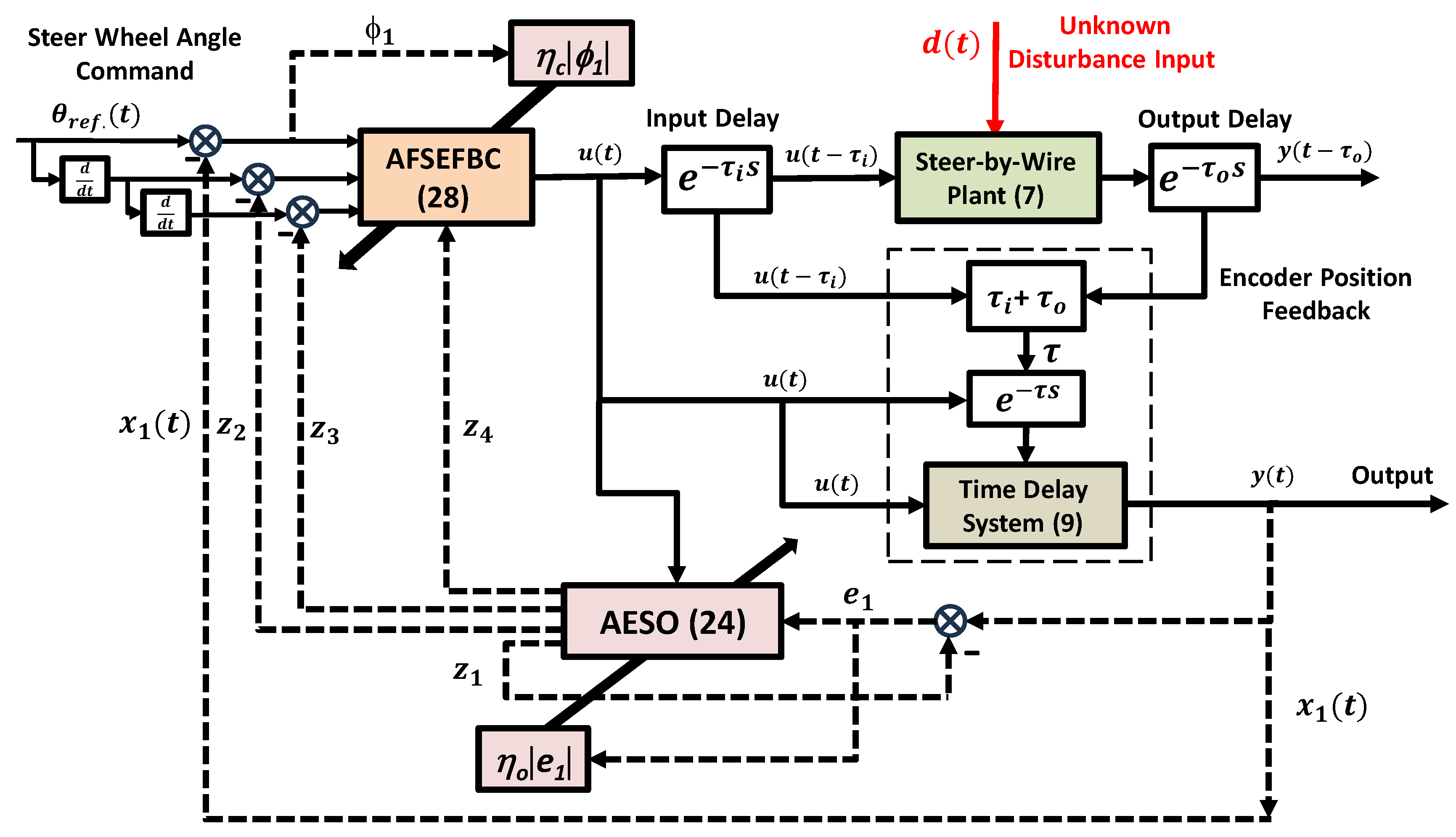
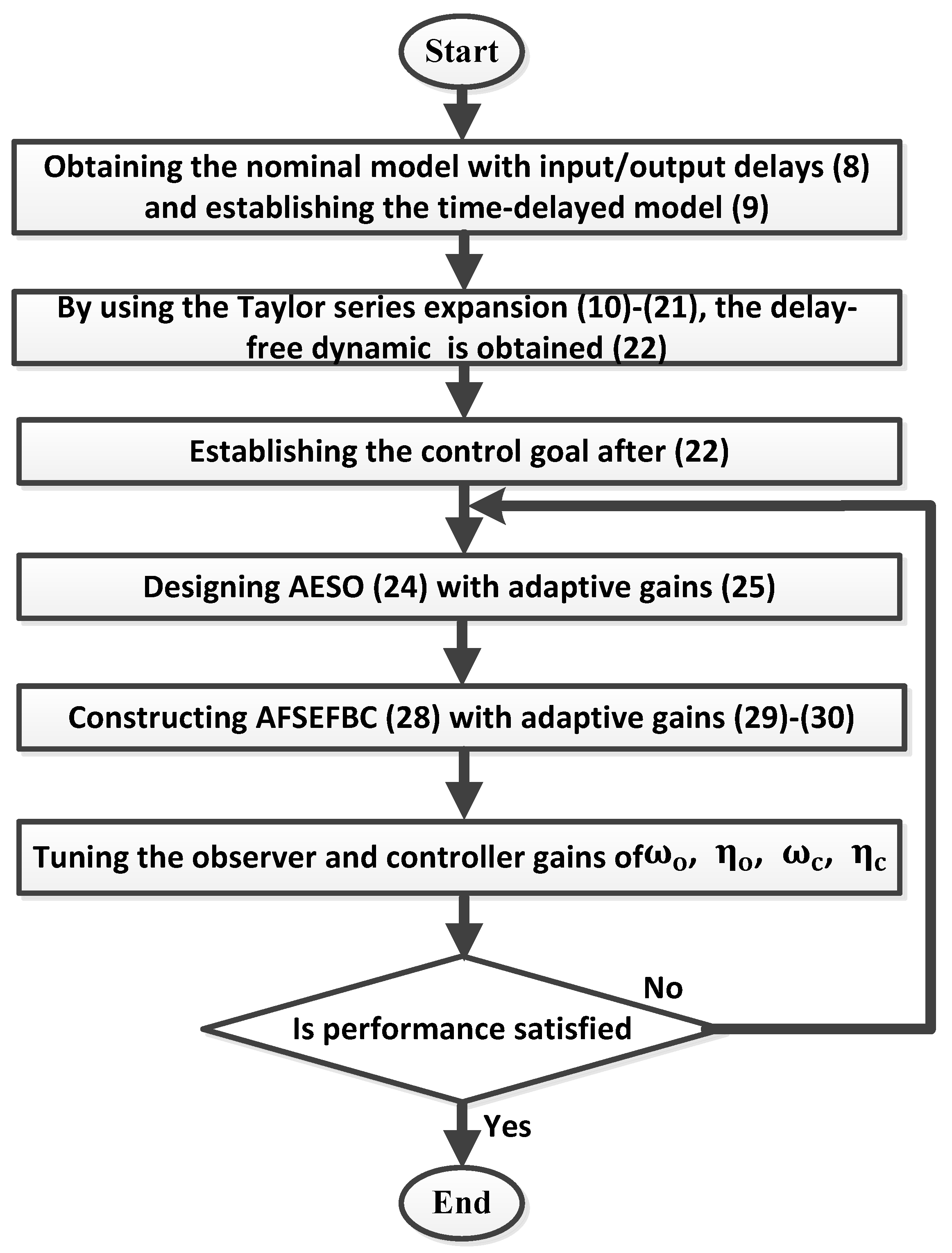
3. Proposed Controller Design and Stability Analysis

In this section, a novel adaptive ADRC (AADRC) approach is established for the time-delayed SBW plant (22), in which the AADRC is constituted from an adaptive full state error feedback control (AFSEFBC) and adaptive extended state observer (AESO). The overall configuration of our designed control scheme is shown in Figure 2, including the AESO and the AFSEFBC, where the adaptive gains of the AESO and the AFESFBC are, respectively, driven by the estimation, and the tracking error of the angular position of SBW dynamics in (8) are constructed to develop the control performance according to [28].

3.1. Construction of the AESO Estimator

In this subsection, the novel AESO is designed for estimating the unmeasured states and the lumped disturbances, ζ ( x , t ) . Defining ζ ( x , t ) as a new extended state x 4 ( t ) with o ( x , t ) ζ ˙ ( x , t ) , nonlinear SBW system (8) is extended as follows:
x ˙ 1 ( t ) = x 2 ( t ) x ˙ 2 ( t ) = x 3 ( t ) x ˙ 3 ( t ) = x 4 ( t ) + f o ( x , t ) + b 0 u ( t ) x ˙ 4 ( t ) = o ( x , t ) .
For the extended system dynamics given in (23), the AESO is designed as
e 1 ( t ) = x 1 ( t ) z 1 ( t ) z ˙ 1 ( t ) = z 2 ( t ) + 4 ω o + g o ( e 1 ( t ) ) e 1 ( t ) z ˙ 2 ( t ) = z 3 ( t ) + 6 ω o + g o ( e 1 ( t ) ) 2 e 1 ( t ) z ˙ 3 ( t ) = z 4 ( t ) + 4 ω o + g o ( e 1 ( t ) ) 3 e 1 ( t ) + b 0 u ( t ) z ˙ 4 ( t ) = ω o + g o ( e 1 ( t ) ) 4 e 1 ( t )
where e 1 ( t ) is the estimation error, z i ( t ) , i = 1 , 2 , 3 , 4 are the estimates of system state x i , i = 1 , 2 , 3 , lumped disturbance x 4 = ζ , and observer bandwidth ω o > 0 . In addition, adaptive gain g ( e 1 ( t ) ) is defined as
g o ( e 1 ( t ) ) = η o | e 1 ( t ) |
where ω o > 0 represents the basic observer bandwidth and η o > 0 is the observer accuracy factor which is used to increase the estimation accuracy of the AESO.

3.2. Construction of AFSEFBC

In this subsection, the AFESFBC is designed to attain satisfactory tracking efficiency. The tracking state error vector of the SBW system, ϕ ( t ) = ϕ 1 ( t ) , ϕ 2 ( t ) , ϕ 3 ( t ) T , is presented by
ϕ 1 ( t ) = y d ( t ) x 1 ( t ) ϕ 2 ( t ) = y ˙ d ( t ) x ˙ 1 ( t ) = y ˙ d ( t ) x 2 ( t ) ϕ 3 ( t ) = y ¨ d ( t ) x ¨ 1 ( t ) = y ¨ d ( t ) x 3 ( t )
where y d stands for the desirable reference signal. Based on (26) and networked time-delayed SBW system (22), the tracking error dynamic is determined as
ϕ ˙ 1 ( t ) = ϕ 2 ( t ) ϕ ˙ 2 ( t ) = ϕ 3 ( t ) ϕ ˙ 3 ( t ) = y d ( t ) f 0 ( t ) b 0 u ( t ) ζ ( x , t ) .
It is noteworthy that the tracking error, ϕ 1 ( t ) , is formally defined in (26), the estimation error, e 1 ( t ) , is precisely delineated in (24), and the lumped uncertainty is exhibited in (6). Furthermore, the lumped uncertainty naturally resides within the plant model, whereas the estimation error serves as the foundation for designing the AESO, and the tracking error is utilized in the design of the AFSEFBC.
According to the AESO (24), the AFSEFBC, u ( t ) , for the dynamical error system in (27) is designed in (24),
u ( t ) = 1 b 0 y d ( t ) + λ 1 ( ϕ 1 ( t ) ) ϕ 1 ( t ) + λ 2 ( ϕ 1 ( t ) ) ϕ ^ 2 ( t ) + λ 3 ( ϕ 1 ( t ) ) ϕ ^ 3 ( t ) f 0 ( z i , t ) z 4 ( t )
where ϕ ^ 2 ( t ) = y ˙ d ( t ) z 2 ( t ) and ϕ ^ 3 ( t ) = y ¨ d ( t ) z 3 ( t ) are, respectively, the estimates of velocity and acceleration tracking error and variables z 2 and z 3 are the states estimated by the AESO. Here, the variable gains are designed as
λ 1 ( ϕ 1 ( t ) ) = ( ω c + g c ( ϕ 1 ( t ) ) ) 3 λ 2 ( ϕ 2 ( t ) ) = 3 ( ω c + g c ( ϕ 1 ( t ) ) ) 2 λ 3 ( ϕ 3 ( t ) ) = 3 ( ω c + g c ( ϕ 1 ( t ) ) )
and
g c ( ϕ 1 ( t ) ) = η c | ϕ 1 ( t ) |
where ω c > 0 is the basic control bandwidth and η c > 0 is the control accuracy factor, which is used to increase the tracking accuracy of the AFSEFBC.
Remark 2.
It is worth pointing out that the proposed adaptive extended state observer AESO in (24) and the proposed adaptive full state error feedback control AFSEFBC (28) work together in the novel adaptive ADRC approach for the time-delayed SBW dynamics. For controlling the steering angle of the SBW as the desired driver hand–wheel angle, the proposed control process starts with preparing the estimation of unmeasured states and the lumped disturbances by the AESO, in which those estimates are required in designing the control law of the AFSEFBC (28). In addition, the AESO is employed to estimate the lumped disturbance that is compensated for in the control law in (28). With the aid of estimations, the proposed AESO-based AFSEFBC is then synthesized to constitute the AADRC scheme, which is used to deal with time-varying disturbances and time delays.
To further help understand the proposed control scheme and ease the practical design process, the corresponding flowchart is presented in Figure 3.

3.3. Stability Proof

This subsection involves the proof of the boundedness of the closed-loop stability under the suggested observer and controller as follows:

3.3.1. Convergence of the AESO

Theorem 1.
Based on Assumption 1 stating that the boundedness of the first derivative of lumped disturbance o = ζ ˙ ( x , t ) is by | o | K 1 , the estimation errors of the AESO are bounded by e K 2 , where K 2 is the positive constant.
Proof of Theorem 1.
With the assistance of extended System Dynamics (23) and AESO Dynamics (24), the estimation error dynamics can be determined as
e ˙ 1 ( t ) = e 2 ( t ) 4 ( ω o + g o ( e 1 ( t ) ) ) e 1 ( t ) e ˙ 2 ( t ) = e 3 ( t ) 6 ( ω o + g o ( e 1 ( t ) ) ) 2 e 1 ( t ) e ˙ 3 ( t ) = e 4 ( t ) 4 ( ω o + g o ( e 1 ( t ) ) ) 3 e 1 ( t ) e ˙ 4 ( t ) = ω o + g o ( e 1 ( t ) ) 4 e 1 ( t ) o ( t )
where e i = x i z i for i = 1 , 2 , 3 , 4 represent the estimations errors. Let us define time-varying observer gains which are a function of the position estimation error as
β 1 ( e 1 ) = 4 ( ω o + g o ( e 1 ( t ) ) ) = 4 ω ¯ o β 2 ( e 1 ) = 6 ( ω o + g o ( e 1 ( t ) ) ) 2 = 6 ω ¯ o 2 β 3 ( e 1 ) = 4 ( ω o + g o ( e 1 ( t ) ) ) 3 = 4 ω ¯ o 3 β 4 ( e 1 ) = ( ω o + g o ( e 1 ( t ) ) ) 4 = ω ¯ o 4
where ω ¯ o > 0 and ω ¯ o ω o . Accordingly, the observer gains in (32) can be rewritten in the vector form as follows:
β 1 ( e 1 ) , β 2 ( e 1 ) , β 3 ( e 1 ) , β 4 ( e 1 ) = 4 ω ¯ o , 6 ω ¯ o 2 , 4 ω ¯ o 3 , ω ¯ o 4 .
Using (33), estimation Error Dynamics (31) can be reformulated by the following compact form:
e ˙ ( t ) = A o e ( t ) + B o o t
where
e = e 1 ( t ) e 2 ( t ) e 3 ( t ) e 4 ( t ) , A o = 4 ω ¯ o 1 0 0 6 ω ¯ o 2 0 1 0 ω ¯ o 3 0 0 1 4 ω ¯ o 4 0 0 0 , B o = 0 0 0 1 .
From (34), we have
e ( t ) = e A o t e ( 0 ) + 0 t e A o ( t τ ) B o o x ( τ ) , τ d τ
where matrix A o is stable Hurwitz, matrix T is invertible real. Accordingly, A o can be expressed by
A o = T diag { ω ¯ o , ω ¯ o , ω ¯ o , ω ¯ o } T 1
where ω ¯ o ( ω ¯ o > 0 ) for i = 1 , 2 , 3 , 4 , stands for the eigenvalues of the proposed AESO.
Then, we have
e A o t = T diag { e ω ¯ o , e ω ¯ o , e ω ¯ o , e ω ¯ o } T 1 .
In addition, using m -norm, the inequality of the exponential of the Hurwitz matrix A o can be given by
e A o t ϕ ( 0 ) e ω ¯ o t
where β is the positive constant.
From (38) and the assumption of | o | K 1 , we can derive the inequality of closed-loop dynamics in (35) as follows:
e A o t e ( 0 ) = e A o t e ( 0 ) + 0 t e A o ( t τ ) B o o x ( τ ) , τ d τ e A o t e ( 0 ) + 0 t e A o ( t τ ) B o o x ( τ ) , τ d τ β e ω ¯ o t e ( 0 ) + B o o x ( τ ) , τ 0 t e A o ( t τ ) β e ω ¯ o t e ( 0 ) + K 1 B o β ω ¯ o ( 1 e ω ¯ o t ) β e ( 0 ) + K 1 B o β ω ¯ o = K 2 .

3.3.2. Convergence of the AFSEFBC

Theorem 2.
We consider that SBW model (8) can track the bounded input reference, x d ( t ) ; if the estimation errors satisfy
lim t e ( t ) = 0
and the adaptive gains are chosen to meet (29), that tracking errors ϕ i for i = 1 , 2 , 3 also converge to zero.
Proof of Theorem 2.
Based on the tracking error trajectories defined in (26), the control effort of the AFSEFBC in (28) is reformulated by
u ( t ) = 1 b 0 y d ( t ) + ε ϕ ( t ) ε e ( t ) f 0 ( z i , t ) ζ ( x , t )
where
ε ϕ ( t ) = λ 1 ( ϕ 1 ( t ) ) ϕ 1 ( t ) + λ 2 ( ϕ 1 ( t ) ) ϕ 2 ( t ) + λ 3 ( ϕ 1 ( t ) ) ϕ 3 ( t ) ε e ( t ) = λ 2 ( ϕ 1 ( t ) ) e 2 ( t ) + λ 3 ( ϕ 1 ( t ) ) e 3 ( t ) e 4 ( t ) .
We let the time-varying controller gains be
λ 1 ( ϕ 1 ) = ( w c + η c | ϕ 1 | ) 3 = w ¯ c 3 λ 2 ( ϕ 1 ) = 3 ( w c + η c | ϕ 1 | ) 2 = 3 w ¯ c 2 λ 3 ( ϕ 1 ) = 3 ( w c + η c | ϕ 1 | ) = 3 w ¯ c
where ω ¯ c > 0 and ω ¯ c ω c . Those gains in (44) can be rewritten as in the following row vector form:
λ 1 ( ϕ 1 ) , λ 2 ( ϕ 1 ) , λ 3 ( ϕ 1 ) = ω ¯ c 3 , 3 ω ¯ c 2 , 3 ω ¯ c
Then, according to (27) and (28), the closed-loop control SBW plant can be expressed as follows:
ϕ ˙ 1 ( t ) = ϕ 2 ( t ) ϕ ˙ 2 ( t ) = ϕ 3 ( t ) ϕ ˙ 3 ( t ) = ε ϕ ( t ) + ε e ( t ) f 0 e ( e , t )
where f 0 e ( e , t ) = f 0 ( x , t ) f 0 ( z , t ) which is presumed to be bounded by | f 0 e ( e , t ) | and the above dynamics can be written in the following compact form:
ϕ ˙ ( t ) = A c ( t ) ϕ ( t ) + B c h c ( t )
where B c = 0 0 1 T , h c ( t ) ε e ( t ) f 0 e ( e , t ) .
A c ( t ) = 0 1 0 0 0 1 ω ¯ c 3 3 ω ¯ c 2 3 ω ¯ c .
From (40), observation errors e i ( t ) , i = 1 , 2 , 3 are bounded; thus, the term c ( t ) is also bounded, and we have
c ( t ) = ε e ( t ) f e 0 ( e , t ) 3 ω ¯ c 2 | e 2 ( t ) | + 3 ω ¯ c | e 3 ( t ) | + | f 0 e ( e , t ) | = c max .
From (45), we have
ϕ ( t ) = e A c t ϕ ( 0 ) + 0 t e A c ( t τ ) B c c e ( τ ) , τ d τ
where A c is also a Hurwitz matrix, thus satisfying
e A t ϕ ( 0 ) β e ω ¯ c t .
As a result, there is the following inequality about ϕ ( t ) :
e A c t ϕ ( 0 ) = e A c t ϕ ( 0 ) + 0 t e A c ( t τ ) B c c e ( τ ) , τ d τ e A c t ϕ ( 0 ) + 0 t e A c ( t τ ) B c c e ( τ ) , τ d τ β e ω ¯ c t ϕ ( 0 ) + B c c e ( τ ) , τ 0 t e A c ( t τ ) β e ω ¯ c t ϕ ( 0 ) + K 2 B c β ω ¯ c ( 1 e ω ¯ c t ) .
On the basis of the assumption given in (40), it can be concluded that the boundedness of ϕ ( t ) is as follows:
lim t ϕ ( t ) = 0 .
From Proof in Section 3.3.1 and Section 3.3.2, with the integration of the AESO and the control action of the AFSEFBC, dynamic closed-loop Tracking Error System (45) is bounded, thus the closed-loop stability dynamic is guaranteed. □
Remark 3.
If g o ( e 1 ( t ) ) = g c ( ϕ 1 ( t ) ) = 0 , the proposed AADRC (28), (24) can be reduced to the well-known ADRC scheme, in which its ESO element is designed as follows:
e 1 ( t ) = x 1 ( t ) z 1 ( t ) z ˙ 1 ( t ) = z 2 ( t ) + 4 ω o e 1 ( t ) z ˙ 2 ( t ) = z 3 ( t ) + 6 ω o 2 e 1 ( t ) z ˙ 3 ( t ) = z 4 ( t ) + 4 ω o 3 e 1 ( t ) + b 0 u ( t ) z ˙ 4 ( t ) = ω o 4 e 1 ( t ) .
In addition, the control law of the FSEFBC with fixed gains is employed as follows:
u ( t ) = 1 b 0 λ 1 ϕ 1 ( t ) + λ 2 ϕ ^ 2 ( t ) + λ 3 ϕ ^ 3 ( t ) z 4 ( t )
in which its gains are tuned according to the following fixed control gains given by
λ 1 = ω c 3 λ 2 = 3 ω c 2 λ 3 = 3 ω c .
The basic ADRC designed in (48) and (49) is used for a comparison purpose that could be fair owing to similar architecture in constructing both proposed AADRC and comparative ADRC. The proposed AADRC approach is expected to perform better than the baseline ADRC in terms of the estimation and tracking performance as discussed in the subsequent section of simulation results.

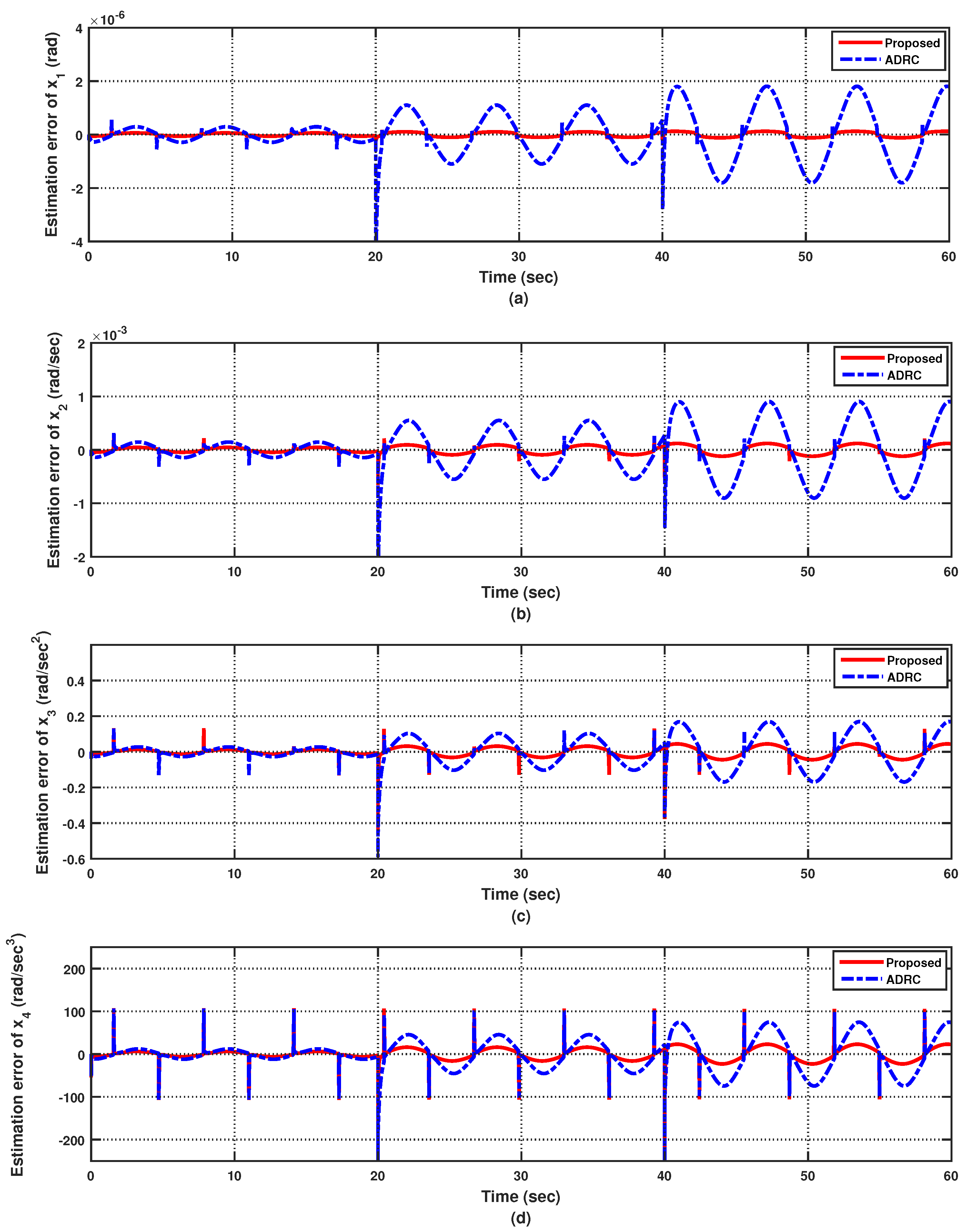
4. Simulation Design and Analysis

To validate the proposed AADRC method, simulations are conducted using MATLAB/SIMULINK 2021. The computer configuration which is utilized for the simulation is presented as follows: i5-2500 CPU @ 3.30 GHz and 4 GB of RAM. The model parameters of the SBW system (1) are detailed in Table 1. Moreover, to demonstrate the superiority of the proposed AFSEFBC with AESO, a comparative analysis, which is conducted between the proposed approach and the benchmark ADRC method [36], is presented in this section. To ensure a fair comparison, both methods utilize an identical sampling time of T s = 4 × 10 3 s. Furthermore, Table 2 provides the tuned controller and observer gains for both the proposed control scheme and the ADRC. Afterward, we detail the simulation outcomes and correlative examinations across two diverse scenarios. In these two cases, the angle of the front wheels is controlled to track a sinusoidal trajectory. It is important to note that, for the sake of comparing the robustness of various controllers, the controller and observer gains are held constant across the two cases. Moreover, both the Coulomb friction torque as expressed in τ c in (1) and the self-aligning torque τ s e l as given in (3) are taken into account in these two cases. To account for the various road conditions throughout the simulation, ρ τ is utilized to determine τ s e l as outlined below:
ρ τ = 155 , 0 < t 20 s , Road with snow 585 , 20 < t 40 s , Road with wet asphalt 960 , 40 < t 60 s , Road with dry asphalt .

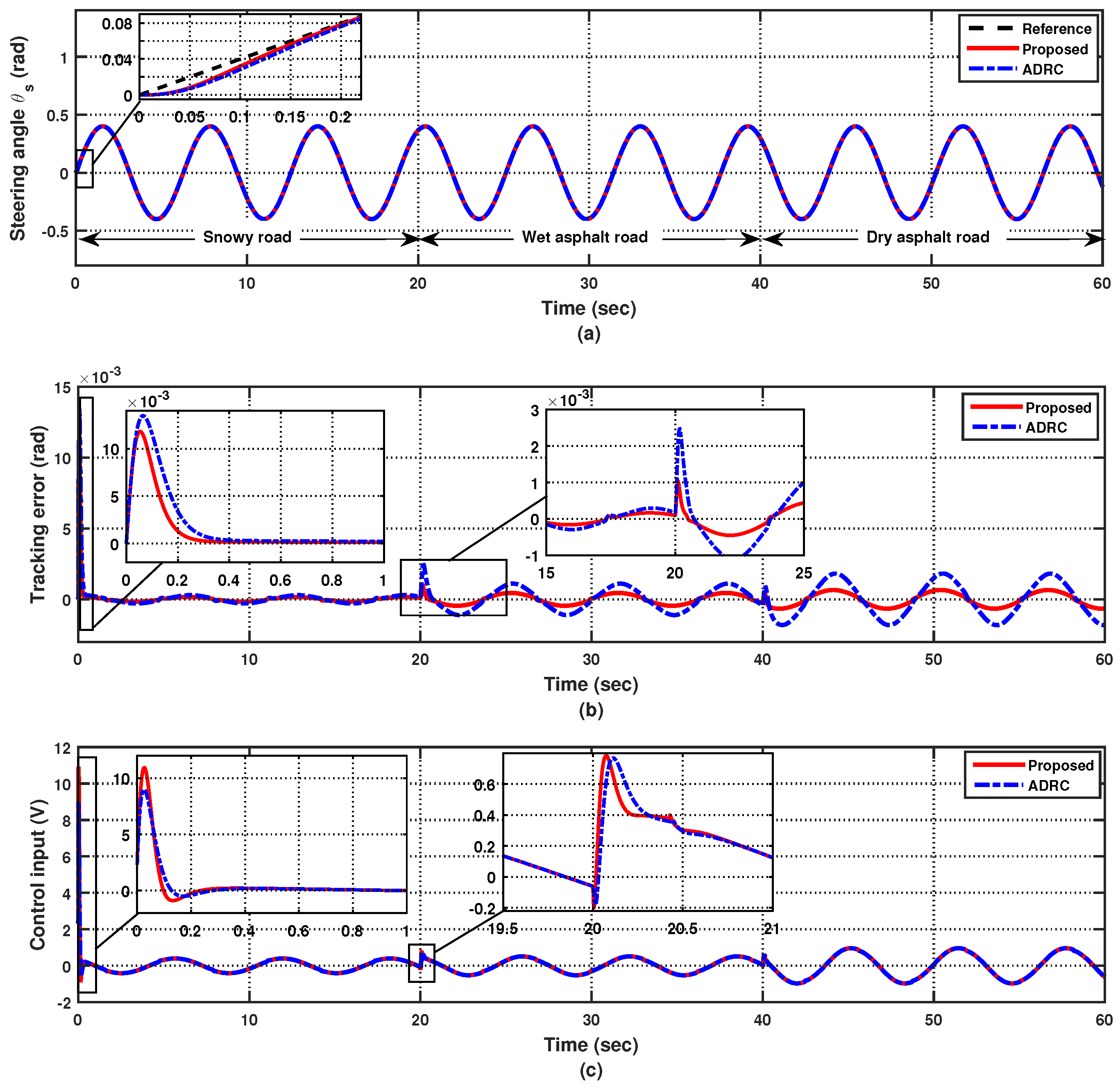
4.1. Case 1: Nominal SBW System with Nonlinearity under the Fixed Input and Output Time Delay

In the first case, the SBW system’s tracking performance is assessed under the nominal nonlinear SBW dynamics in the presence of fixed communication time delays. To investigate this case, both the parametric uncertainties as expressed in (2) and external disturbance d ( t ) as given in (5) are set to zero. Furthermore, the input and output time delays as illustrated in Figure 1 are assigned values of τ i = 5 × 10 3 s and τ o = 5 × 10 3 s, respectively. Thus, the sum of τ i and τ o matches the sampling time T s . In Figure 4a–d, the estimation errors for x 1 , x 2 , x 3 , and x 4 are presented, highlighting the superior estimation performance of the proposed algorithm when compared to the benchmark ADRC method. It is evident that estimation errors x 1 , x 2 , x 3 , and x 4 of the proposed algorithm are lower than those of the comparison approach. In addition, the estimation error in the proposed approach converges faster. Moreover, it is observed that some spikes occur in the estimation errors in both methods due to the observer gains’ dependency on the discrepancy between x 1 and its estimation. Nevertheless, the AESO exhibits a faster convergence rate compared to the ESO in the comparative method, with estimation errors being smaller in the proposed approach. In Figure 5a–c, the trajectories of steering angle θ s , the tracking error of θ s , and control input u ( t ) are displayed under both the proposed algorithm and the comparative method. In Figure 5a,b, it is evident that the convergence rate achieved under the proposed control method outperforms that of the ADRC. Furthermore, the tracking error in the proposed algorithm is reduced, as the impact of time delays is effectively mitigated by the AESO in the proposed control approach. In addition, Figure 5c clearly illustrates that the proposed control approach exhibits a more expeditious response in the control input when compared to the ADRC. To achieve a comprehensive understanding of the proposed control scheme, Figure 6a,b presents adaptive gain k c of the AGSEFBC and adaptive gain k o of the AESO, respectively, along with the corresponding fixed gains of ESO in the ADRC. By comparing Figure 4a and Figure 6a, Figure 5b and Figure 6b, it can be observed that adaptive gains k c and k o vary in response to the estimation error of x 1 and the tracking error of θ s , respectively. In contrast, it is evident that the gains in the ADRC remain fixed, as illustrated in Figure 6a,b.

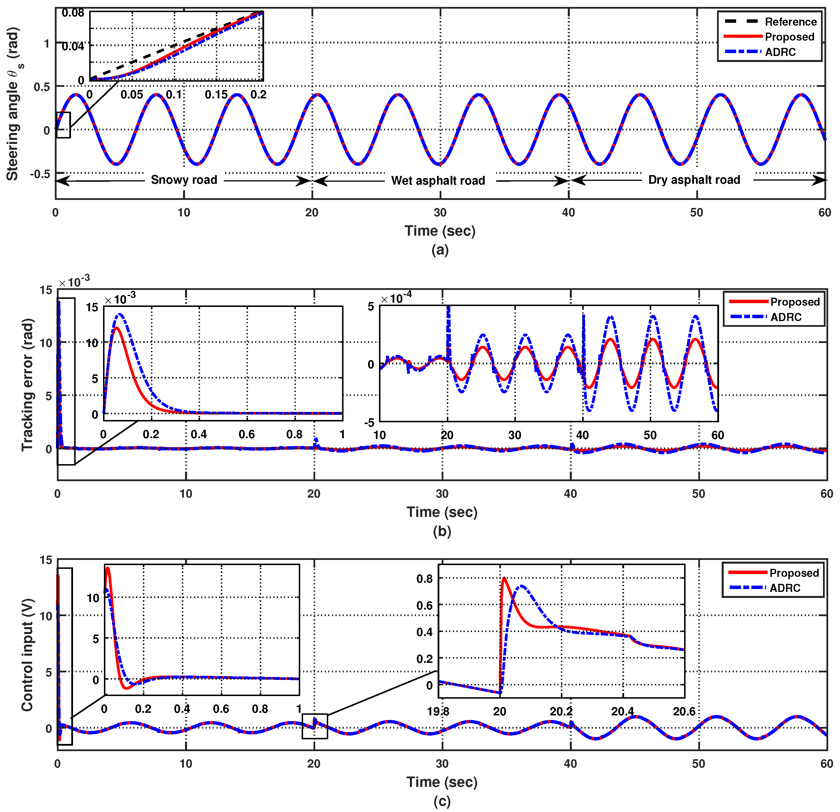
4.2. Case 2: Uncertain SBW System with Nonlinearity under Input and Output Time-Varying Delay

In comparison to Case 1, parameter uncertainties such as inertia, damping, and Coulomb fraction variations are newly considered in Case 2, which are specified in (2). Accordingly, the inertia, damping, and Coulomb fraction variations are formulated by Δ ¯ J e = 0.1 J e 0 , Δ ¯ B e = 0.1 B e 0 , and Δ ¯ ξ f = 0.1 ξ f 0 , respectively, as in (2). In addition, the external disturbance acting on the SBW dynamics modeled in (5) is defined by d ( t ) = sin ( t ) . The time-varying communication delays consist of a fixed component, i.e., τ i = 2 × 10 2 s for the control input and τ o = 2 × 10 2 s for the front wheels’ angle feedback, and a varying component with an upper bound of 5 × 10 3 for both input and out delays. Please note that the sum of the input and output delays significantly exceeds sampling time T s in Case 2. In Figure 7a–d, the estimation errors for x 1 , x 2 , x 3 , and x 4 are depicted. In Case 2, we notice that the performance of the proposed algorithm consistently surpasses the ADRC with respect to estimation, as it exhibits a quicker convergence rate and smaller estimation errors even under large time delays. In Figure 8a–c, it is clear that the tracking error of θ s in the proposed control remains smaller than that of the ADRC. Furthermore, the convergence rate of the tracking error and the response rate of the control input in the proposed control are faster than the comparative ADRC. By comparing Figure 7a and Figure 9a, Figure 8b and Figure 9b, it can be observed that adaptive gains k c and k o in Case 2 exhibit a broader range than those in Case 1 to counteract the existence of parameter uncertainties, external disturbance, and significant time-varying delays. Thus, the adaptive gains in the proposed AADRC scheme can adaptively update to maintain good performance, whereas the estimation and tracking performance of the ADRC are not as good as the proposed one due to the ADRC’s fixed controller and observer gains.
To sum up, it is worth mentioning from Cases 1 and 2 that adaptive mechanisms used in (25) and (30) are, respectively, used to update gains of Observer (24) and Controller (28) elements, which play a focal role in contributing and improving not only the peaking reduction in transient region and the accuracy steady as shown in Figure 5b and Figure 8b. The reason for the adaptive mechanisms’ contribution is that the adaptive gains of both the proposed observer and controller are, respectively, functions of the estimation and tracking errors, in which those gains increase when the errors become bigger and vice versa. As depicted in Figure 6 and Figure 9, both the proposed observer and controller gains increase largely in the transient region to compensate for the peaking phenomenon in the estimation and tracking trajectories in that region. In addition, those gains continue increasing at different times in the steady-state region, especially when the errors occur largely in that region, leading to the enhancement of observation and tracking accuracy. Furthermore, these adaptively increased gains bring strong robustness as demonstrated in Case 2 compared to the well-known ADRC with fixed gains.
Consequently, according to the results extracted from Cases 1 and 2, the advantages of the proposed AADRC methodology are highlighted by and summarized into the following: (1) Better estimation accuracy with a lesser peak pheromone of the estimated states, uncertainties, and disturbances; even the time-delayed SWB order increases by one due to the use of Taylor transformation; (2) Strong robustness in effectively handling not only the detrimental effects of the parametric uncertainties, nonlinearities, and external disturbances but also input and output time delays induced from the networked control SBW system and variations in those time delays; and (3) Improvement in the transient and steady-state performances of the output tracking trajectory of the SWB system with time-delay communications.

5. Conclusions

In this paper, the novel AADRC scheme is designed for the SBW with disturbances and time delays induced by the transmission channel to improve the transient rate and steady-state tracking accuracy of the steer angle performance. To diminish the impacts of large time delays in communication, Taylor series expansion is employed for the time-delayed second-order SBW system. Then, the impact of not only uncertainties, disturbances, and time delays is diminished, but also the increased order by the Taylor transformation is well dealt with by the proposed AADRC approach. The novel AADRC scheme comprises the AESO and AFSEFBC elements. First, the AESO is built to observe unmeasured velocity, acceleration states, and the lumped disturbance, in which adaptive gains of the AESO are varied online according to the estimation error of the steering angle to minimize the peaking of the estimation. Second, the AFSEFBC is constructed to attain steering tracking control, in which its gains are driven depending on the tracking error of the steering angle. Finally, the convergence and boundedness analysis of the closed-loop dynamics of both the AESO and AFSEFBC are mathematically presented in the presence of large time delays and unknown disturbances. Simulation outcomes verify the superiority of the proposed control algorithm in comparison to the well-known ADRC technique with fixed gains.
Future research should focus on the potential applications of the proposed control strategy to other x-by-wire technologies (i.e., x-by-wire including drive/brake-by-wire systems) with time delays induced from the NCSs and other automobile applications, such as automobile electronic throttle systems subject to more sophisticated probability density function distribution disturbances describing the influence of uncertainty propagation on those systems. More specifically, despite the challenges associated with obtaining an accurate mathematical representation of lumped uncertainty in practice, we can still leverage statistical methods to model this uncertainty as a random input to the system. Utilizing probability density functions, we can approximate and analyze the corresponding system output triggered by this uncertainty [37].

Author Contributions

Conceptualization, K.R., Z.C. and Z.M.; methodology, K.R. and Z.C.; software, K.R.; validation, K.R., Y.Z., Z.C. and Z.M.; formal analysis, K.R. and Y.Z.; investigation, K.R., Z.C. and Y.Z.; resources, Z.C. and Z.M.; writing—original draft preparation, Y.Z. and K.R.; writing—review and editing, K.R., Y.Z., Z.C. and Z.M.; visualization, Y.Z., K.R., Z.C. and Z.M.; supervision, Z.C. and Z.M.; project administration, Z.C. All authors have read and agreed to the published version of the manuscript.

Funding

This work was supported in part by the Australian Research Council Discovery Project under Grant DP190101557.

Informed Consent Statement

Not applicable.

Data Availability Statement

Data sharing is not applicable to this article.

Acknowledgments

Kamal Rsetam would like to appreciate the Republic of Iraq/Ministry of Higher Education and Scientific Research and the University of Baghdad/Al Khwarizmi College of Engineering for granting a Research Fellowship.

Conflicts of Interest

The authors declare no conflicts of interest.

References

  1. Wang, H.; Man, Z.; Shen, W.; Cao, Z.; Zheng, J.; Jin, J.; Tuan, D. Robust Control for Steer-by-Wire Systems With Partially Known Dynamics. IEEE Trans. Ind. Inform. 2014, 10, 2003–2015. [Google Scholar] [CrossRef]
  2. Sun, Z.; Zheng, J.; Man, Z.; Wang, H. Robust control of a vehicle steer-by-wire system using adaptive sliding mode. IEEE Trans. Ind. Electron. 2015, 63, 2251–2262. [Google Scholar] [CrossRef]
  3. Zhang, G.; Wang, X.; Li, L.; Shao, W. Design and applications of steering angle tracking control with robust compensator for steer-by-wire system of intelligent vehicle. IFAC-PapersOnLine 2021, 54, 221–227. [Google Scholar] [CrossRef]
  4. Shi, Q.; He, S.; Wang, H.; Stojanovic, V.; Shi, K.; Lv, W. Extended state observer based fractional order sliding mode control for steer-by-wire systems. IET Control Theory Appl. 2023. [Google Scholar] [CrossRef]
  5. Ye, Q.; Wang, R.; Cai, Y.; Chadli, M. The stability and accuracy analysis of automatic steering system with time delay. ISA Trans. 2020, 104, 278–286. [Google Scholar] [CrossRef]
  6. Yang, J.; Chen, W.; Li, S.; Guo, L.; Yan, Y. Disturbance/Uncertainty Estimation and Attenuation Techniques in PMSM Drives—A Survey. IEEE Trans. Ind. Electron. 2017, 64, 3273–3285. [Google Scholar] [CrossRef]
  7. Xiong, L.; Jiang, Y.; Fu, Z. Steering Angle Control of Autonomous Vehicles Based on Active Disturbance Rejection Control. IFAC-PapersOnLine 2018, 51, 796–800. [Google Scholar] [CrossRef]
  8. Sun, Z.; Zheng, J.; Man, Z.; Wang, H.; Lu, R. Sliding mode-based active disturbance rejection control for vehicle steer-by-wire systems. IET Cyber-Phys. Syst. Theory Appl. 2018, 3, 1–10. [Google Scholar] [CrossRef]
  9. Wang, H.; Xu, Z.; Do, M.; Zheng, J.; Cao, Z.; Xie, L. Neural-network-based robust control for steer-by-wire systems with uncertain dynamics. Neural Comput. Appl. 2015, 26, 1575–1586. [Google Scholar] [CrossRef]
  10. Zhang, J.; Wang, H.; Ma, M.; Yu, M.; Yazdani, A.; Chen, L. Active front steering-based electronic stability control for steer-by-wire vehicles via terminal sliding mode and extreme learning machine. IEEE Trans. Veh. Technol. 2020, 69, 14713–14726. [Google Scholar] [CrossRef]
  11. Benosman, M. Model-based vs data-driven adaptive control: An overview. Int. J. Adapt. Control Signal Process. 2018, 32, 753–776. [Google Scholar] [CrossRef]
  12. Sun, Z.; Zheng, J.; Wang, H.; Man, Z. Adaptive fast non-singular terminal sliding mode control for a vehicle steer-by-wire system. IET Control Theory Appl. 2017, 11, 1245–1254. [Google Scholar] [CrossRef]
  13. Ye, M.; Wang, H. Robust adaptive integral terminal sliding mode control for steer-by-wire systems based on extreme learning machine. Comput. Electr. Eng. 2020, 86, 106756. [Google Scholar] [CrossRef]
  14. Wu, J.; Zhang, J.; Nie, B.; Liu, Y.; He, X. Adaptive Control of PMSM Servo System for Steering-by-Wire System With Disturbances Observation. IEEE Trans. Transp. Electrif. 2022, 8, 2015–2028. [Google Scholar] [CrossRef]
  15. Iqbal, J.; Zuhaib, K.; Han, C.; Khan, A.; Ali, M. Adaptive Global Fast Sliding Mode Control for Steer-by-Wire System Road Vehicles. Appl. Sci. 2017, 7, 738. [Google Scholar] [CrossRef]
  16. Yang, H.; Liu, W.; Li, C.; Fan, Y. An adaptive hierarchical control approach of vehicle handling stability improvement based on Steer-by-Wire Systems. Mechatronics 2021, 77, 102583. [Google Scholar] [CrossRef]
  17. Wang, Y.; Luo, G.; Wang, D. Observer-based fixed-time adaptive fuzzy control for SbW systems with prescribed performance. Eng. Appl. Artif. Intell. 2022, 114, 105026. [Google Scholar] [CrossRef]
  18. Shukla, H.; Roy, S.; Gupta, S. Robust Adaptive Control of Steer-by-wire Systems under Unknown State-dependent Uncertainties. Int. J. Adapt. Control Signal Process. 2022, 36, 198. [Google Scholar] [CrossRef]
  19. Wang, H.; Man, Z.; Kong, H.; Zhao, Y.; Yu, M.; Cao, Z.; Zheng, J.; Do, M.T. Design and implementation of adaptive terminal sliding-mode control on a steer-by-wire equipped road vehicle. IEEE Trans. Ind. Electron. 2016, 63, 5774–5785. [Google Scholar] [CrossRef]
  20. Shah, M.B.N.; Husain, A.R.; Aysan, H.; Punnekkat, S.; Dobrin, R.; Bender, F.A. Error handling algorithm and probabilistic analysis under fault for CAN-based steer-by-wire system. IEEE Trans. Ind. Inform. 2016, 12, 1017–1034. [Google Scholar] [CrossRef]
  21. Zhang, B.; Zhao, W.; Wang, C.; Lian, Y. Layered Time-delay Robust Control Strategy for Yaw Stability of SBW Vehicles. IEEE Trans. Intell. Veh. 2023; early access. [Google Scholar]
  22. Chuei, R.; Zheng, Y.; Cao, Z.; Man, Z. Improved sliding mode observer based repetitive control for linear systems with time-varying input and state delays. Int. J. Adapt. Control. Signal Process. 2023; early access. [Google Scholar]
  23. Lu, Y.; Liang, J.; Wang, F.; Yin, G.; Pi, D.; Feng, J.; Liu, H. An active front steering system design considering the CAN network delay. IEEE Trans. Transp. Electrif. 2023, 9, 5244–5256. [Google Scholar] [CrossRef]
  24. Yang, Y.; Yan, Y.; Xu, X. Fractional order adaptive fast super-twisting sliding mode control for steer-by-wire vehicles with time-delay estimation. Electronics 2021, 10, 2024. [Google Scholar] [CrossRef]
  25. Chakirov, R.; Vagapov, Y.; Gaede, A. Active sidestick for steer-by-wire systems. J. Electr. Electron. Eng. 2010, 3, 43–46. [Google Scholar]
  26. Paolo, P.; Peter, M.; Norah, N. Fluid Interface Concept for Automated Driving. HCI Mobil. Transp. Automot. Syst. Autom. Driv. In-Veh. Exp. Des. 2020, 12212, 114–115. [Google Scholar]
  27. Mortazavizadeh, S.; Ghaderi, A.; Ebrahimi, M.; Hajian, M. Recent Developments in the Vehicle Steer-by-Wire System. IEEE Trans. Transp. Electrif. 2020, 6, 1226–1235. [Google Scholar] [CrossRef]
  28. Chen, B.M.; Lee, T.H.; Peng, K.; Venkataramanan, V. Composite nonlinear feedback control for linear systems with input saturation: Theory and an application. IEEE Trans. Autom. Control 2003, 48, 427–439. [Google Scholar] [CrossRef]
  29. Yih, P.; Gerdes, J.C. Modification of vehicle handling characteristics via steer-by-wire. IEEE Trans. Control Syst. Technol. 2005, 13, 965–976. [Google Scholar] [CrossRef]
  30. Rajamani, R. Vehicle Dynamics and Control; Springer: New York, NY, USA, 2012. [Google Scholar]
  31. Wang, H.; Kong, H.; Man, Z.; Cao, Z.; Shen, W. Sliding mode control for steer-by-wire systems with AC motors in road vehicles. IEEE Trans. Ind. Electron. 2013, 61, 1596–1611. [Google Scholar] [CrossRef]
  32. Baviskar, A.; Wagner, J.R.; Dawson, D.M.; Braganza, D.; Setlur, P. An adjustable steer-by-wire haptic-interface tracking controller for ground vehicles. IEEE Trans. Veh. Technol. 2008, 58, 546–554. [Google Scholar] [CrossRef]
  33. Wu, Q.; Yu, L.; Wang, Y.W.; Zhang, W.A. LESO-based position synchronization control for networked multi-axis servo systems with time-varying delay. IEEE/CAA J. Autom. Sin. 2020, 7, 1116–1123. [Google Scholar] [CrossRef]
  34. Li, P.; Zhu, G.; Zhang, M. Linear Active Disturbance Rejection Control for Servo Motor Systems With Input Delay via Internal Model Control Rules. IEEE Trans. Ind. Electron. 2021, 68, 1077–1086. [Google Scholar] [CrossRef]
  35. Cao, W.; Wang, L.; Li, J.; Peng, C.; Zhou, J.; He, H. Analysis and Design of Drivetrain Control for the AEV With Network-Induced Compounding-Construction Loop Delays. IEEE Trans. Veh. Technol. 2021, 70, 5578–5591. [Google Scholar] [CrossRef]
  36. Han, J. From PID to Active Disturbance Rejection Control. IEEE Trans. Ind. Electron. 2009, 56, 900–906. [Google Scholar] [CrossRef]
  37. Zhang, Z.; Wang, J.; Jiang, C.; Huang, Z. A new uncertainty propagation method considering multimodal probability density functions. Struct. Multidiscip. Optim. 2019, 60, 1983–1999. [Google Scholar] [CrossRef]
Figure 1. Schematic SBW system with communication time delays.
Asi 07 00022 g001
Figure 2. Configuration of the proposed AADRC for the SBW system.
Asi 07 00022 g002
Figure 3. Flowchart of the proposed AADRC scheme.
Asi 07 00022 g003
Figure 4. Estimation error responses for the nominal system with nonlinearity under the input time delay, τ i = 5 × 10 3 s, and the output time delay, τ o = 5 × 10 3 s (Case 1).
Asi 07 00022 g004
Figure 5. Tracking responses for the nominal system with nonlinearity under the input time delay, τ i = 5 × 10 3 s, and the output time delay, τ o = 5 × 10 3 s (Case 1).
Asi 07 00022 g005
Figure 6. Adaptive gains (where k o = ω ¯ o , k c = ω ¯ c ) of the proposed scheme for the nominal system under input delay τ i = 5 × 10 3 s and output delay τ o = 5 × 10 3 s (Case 1).
Asi 07 00022 g006
Figure 7. Estimation error responses for the uncertain system under the input time delay, τ i = 2 × 10 2 s, the output time delay, τ o = 2 × 10 2 s, and delay variation Δ τ = 5 × 10 3 s (Case 2).
Asi 07 00022 g007
Figure 8. Tracking responses for the uncertain system under the input time delay, τ i = 2 × 10 2 s, the output time delay, τ o = 2 × 10 2 s, and delay variation Δ τ = 5 × 10 3 s (Case 2).
Asi 07 00022 g008
Figure 9. Adaptive gains (where k o = ω ¯ o , k c = ω ¯ c ) of the proposed scheme for the uncertain system under the input delay, τ i = 2 × 10 2 s, output delay τ o = 2 × 10 2 s, and delay variation Δ τ = 5 × 10 3 s (Case 2).
Asi 07 00022 g009
Table 1. Value of the SBW system.
SymbolsDescriptionsValuesUnits
J e Equivalent inertial moment of the SBW system85.5kgm2
B e Equivalent viscous damping friction of the SBW system218.8Nms/rad
ξ f Coulomb friction constant4.2Nm
κ 1 Scale factor to account for transmitting from the linear motion of the rack to the steering angle of front wheels6.0-
κ 2 Gear ratio between the pinion and rack system3.0-
κ 3 Gear ratio of the gear head8.5-
κ 4 Scale factor accounting for converting from the input voltage of steering motor to the output torque of the steering motor1.8-
Table 2. Parameters of Control Schemes in All Cases.
ControlProposedADRC
Parameters(24)–(28)(48) and (49)
ω c 2525
k c 700-
ω o 125125
k o 1 × 10 9 -
Disclaimer/Publisher’s Note: The statements, opinions and data contained in all publications are solely those of the individual author(s) and contributor(s) and not of MDPI and/or the editor(s). MDPI and/or the editor(s) disclaim responsibility for any injury to people or property resulting from any ideas, methods, instructions or products referred to in the content.

