
A Comparison of Three Simulation Techniques for Modeling the Fan Blade–Composite Abradable Rub Strip Interaction in Turbofan Engines

Abstract
:
1. Introduction
2. Metrics for the Description of the Blade–ARS Interaction
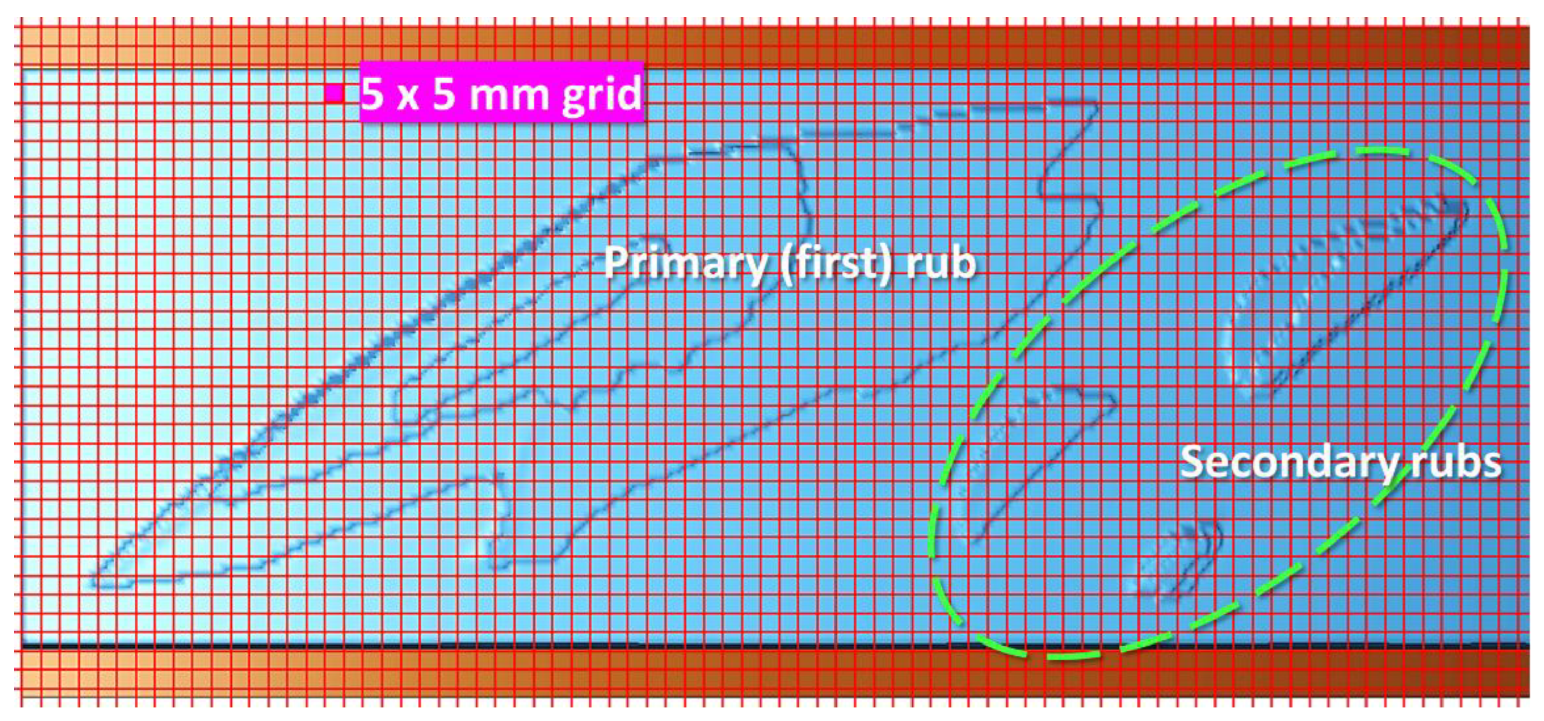
2.1. Rub Morphology
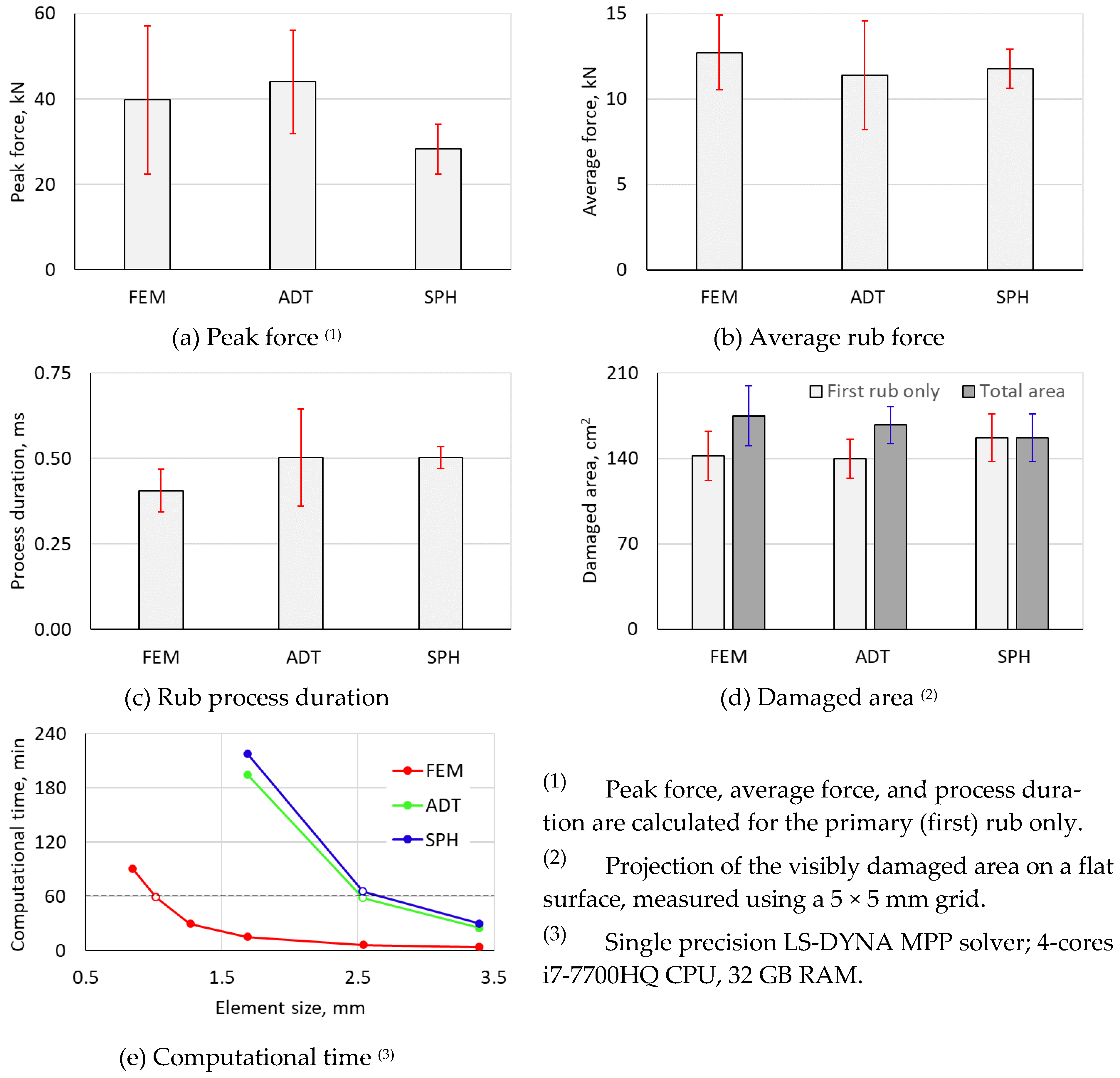
2.2. Damaged Area
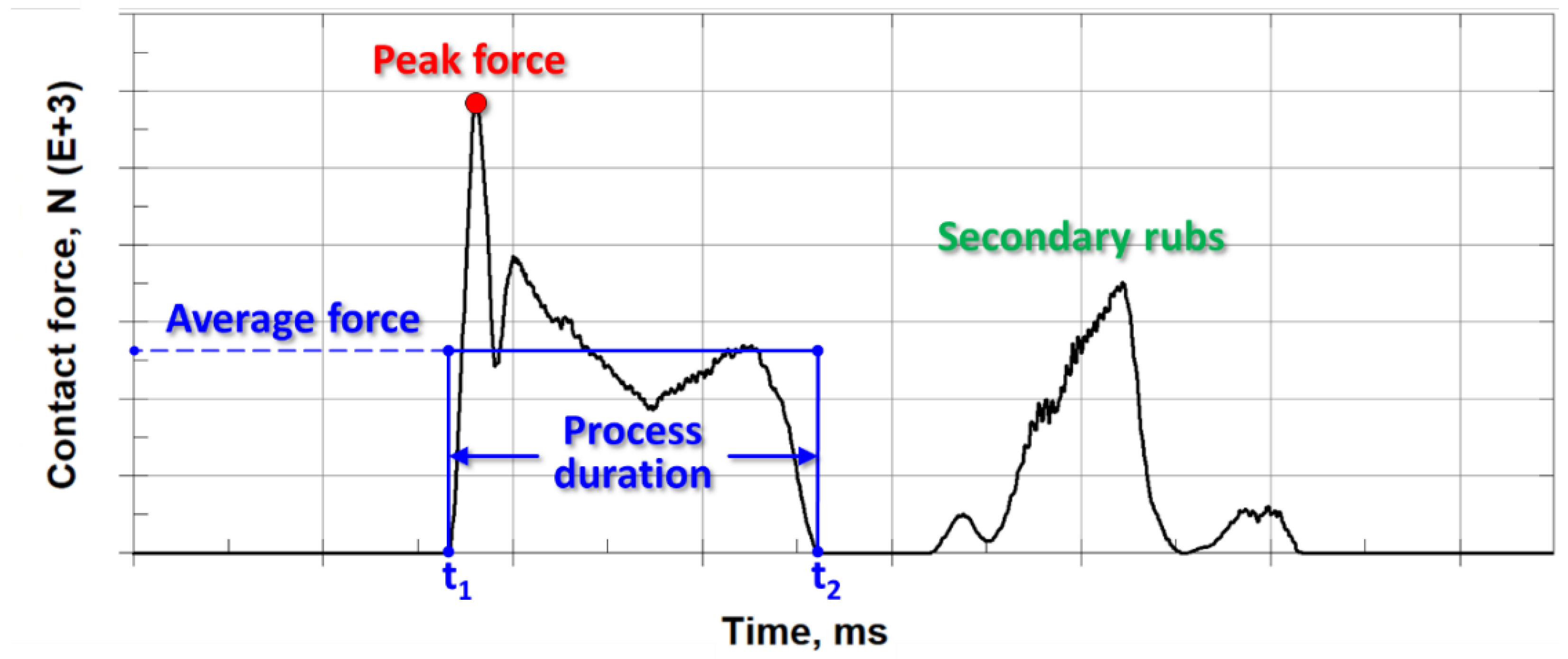
2.3. Peak Force
2.4. Process Duration
2.5. Average Force
3. Material Modeling
3.1. Experimental Observations and Modeling Implications
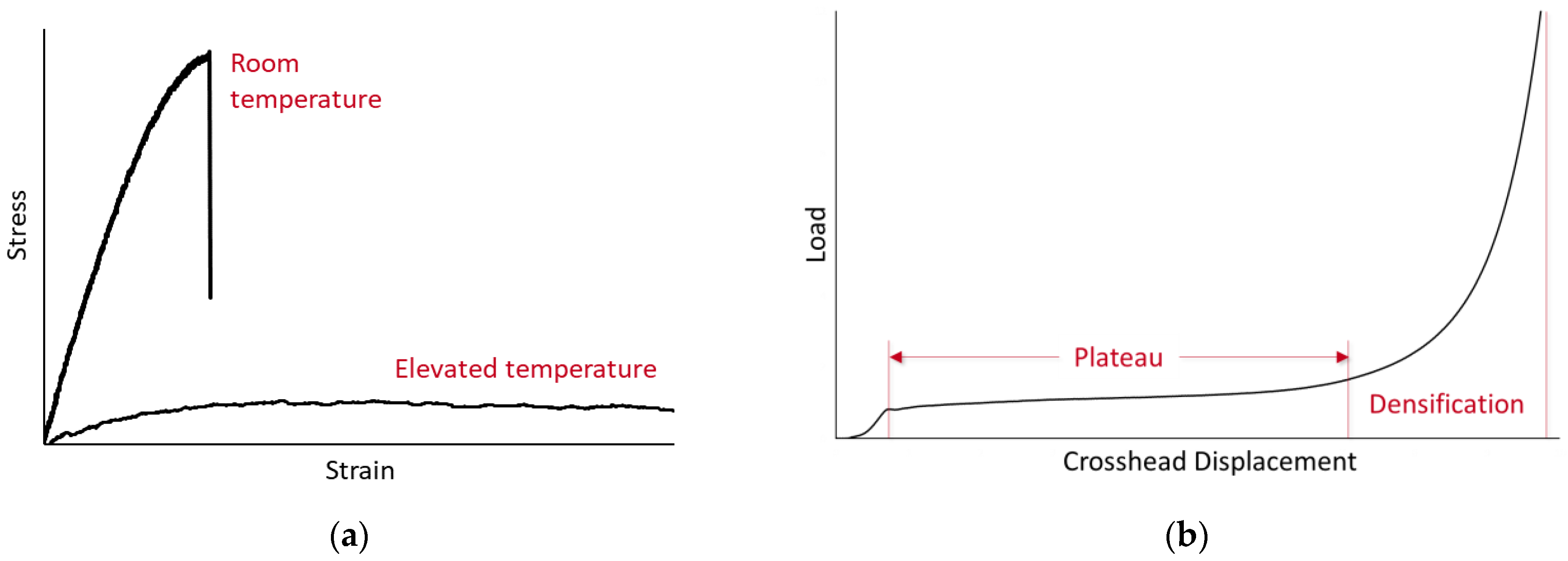
- Temperature dependence of properties, owing to the known influence of heat on the behavior of polymers (softening, plasticization). Experimental uniaxial tension curves for an abradable rub strip material at room temperature (RT) and an elevated temperature (ET) corresponding to the glass transition region of its polymer matrix are shown in Figure 5a. As can be deduced from the figure, at ET the material exhibits nearly elastic–perfectly plastic behavior with the strength of only a fraction of its RT value. Near or above Tg, the abradable strength drops to “structurally insignificant” values, usually of the order of only a few megapascals.
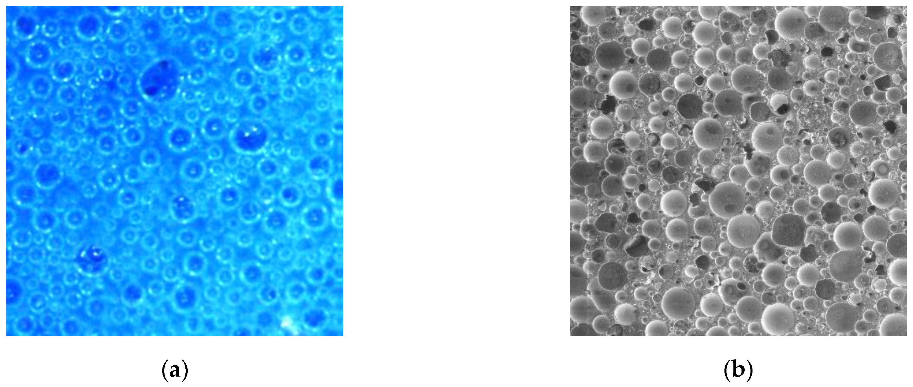
- Compaction under compressive loading, due to the progressive collapse of hollow glass microspheres, resulting in significant volume changes until densification. An experimental curve depicting the behavior of an abradable under confined compression loading is shown in Figure 5b. The pore collapse corresponds to the plateau stage on the curve.
3.2. Strength Model
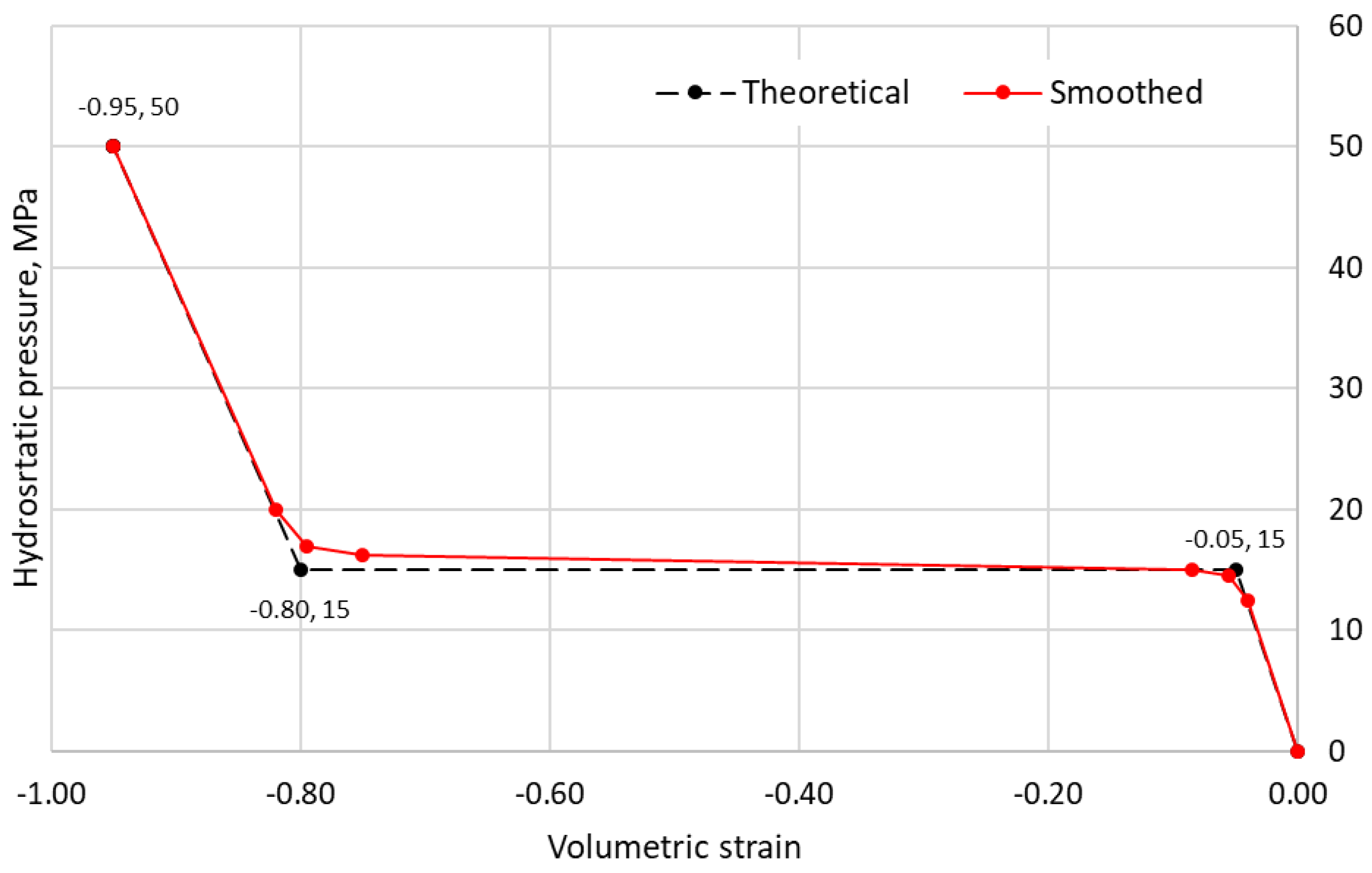
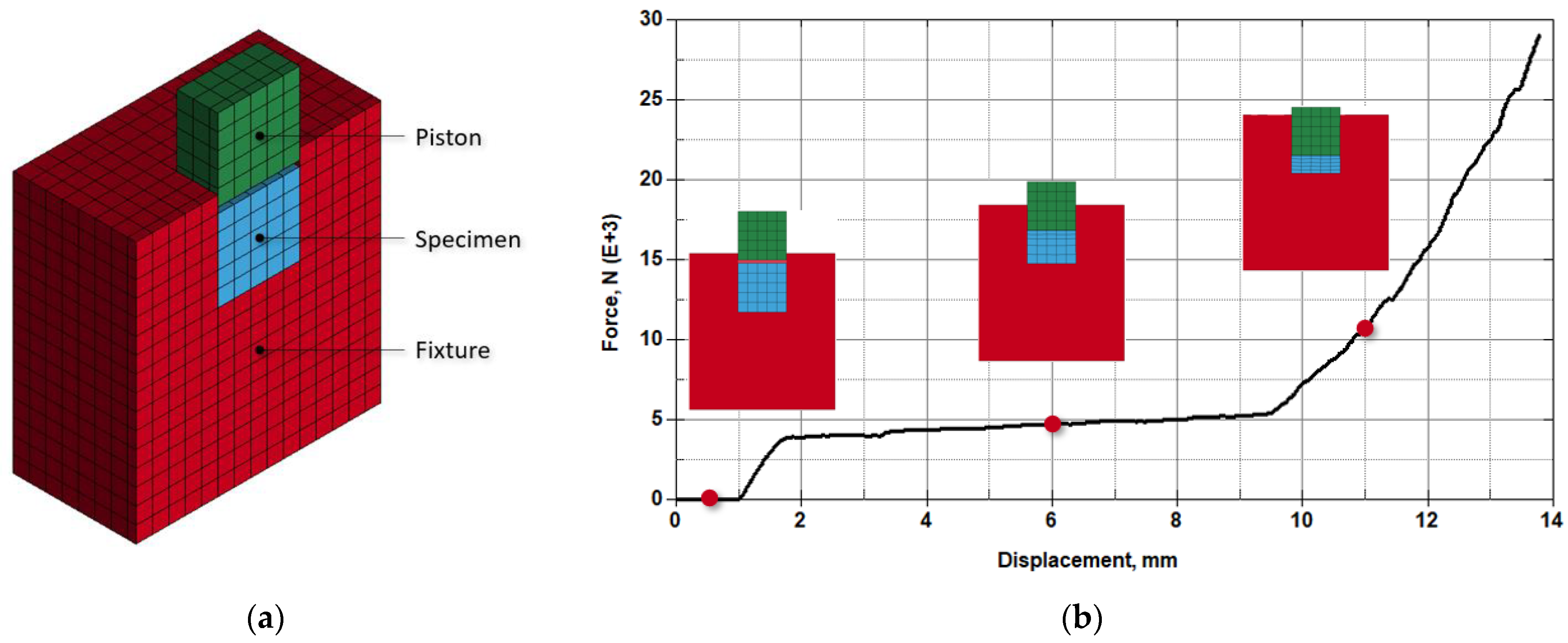
3.3. Equation of State
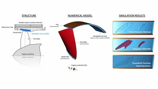
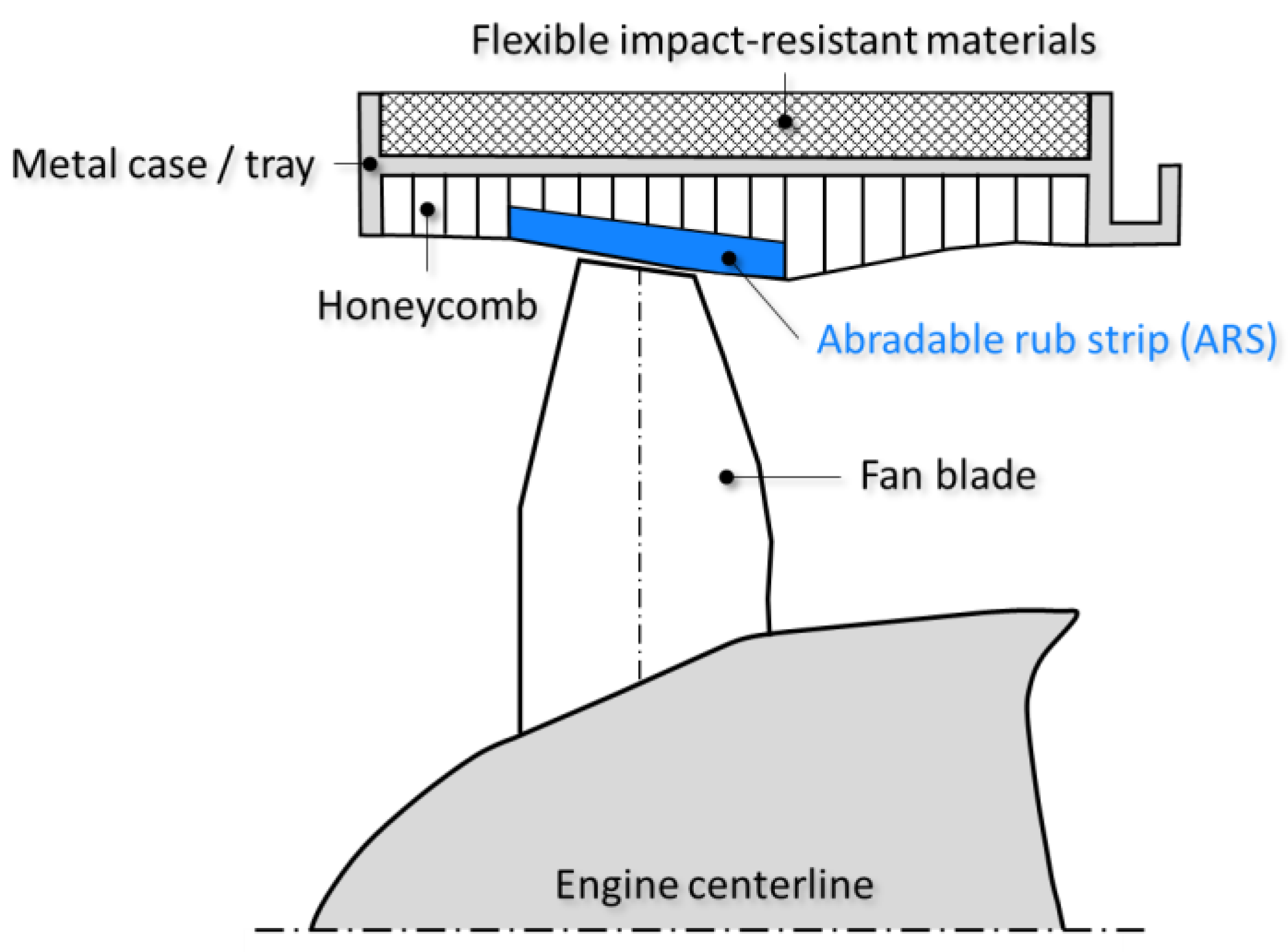
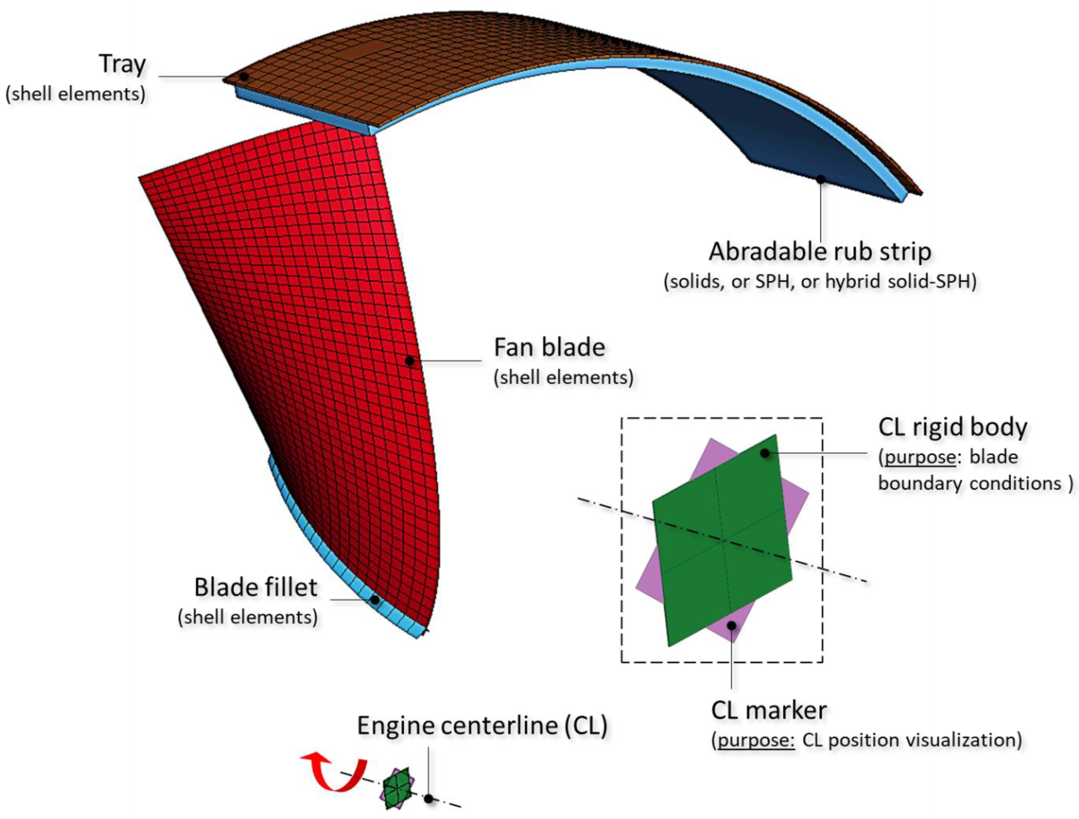
4. Simulation Model
4.1. General Description
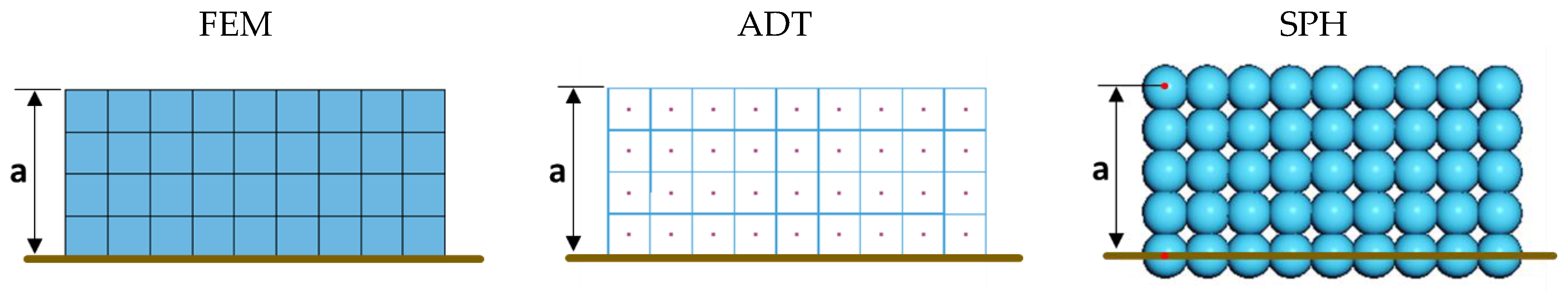
4.2. Numerical Schemes
- Finite Element Method (FEM) with the element erosion. This approach usually provides a good balance between simulation accuracy and computational efficiency in impact problems; however, its applicability may vary depending on the levels of deformation experienced by elements in simulations. In addition, identifying erosion strain—a non-physical parameter determining the upper limit of deformation that an element can tolerate before removal from simulation—is often non-trivial.
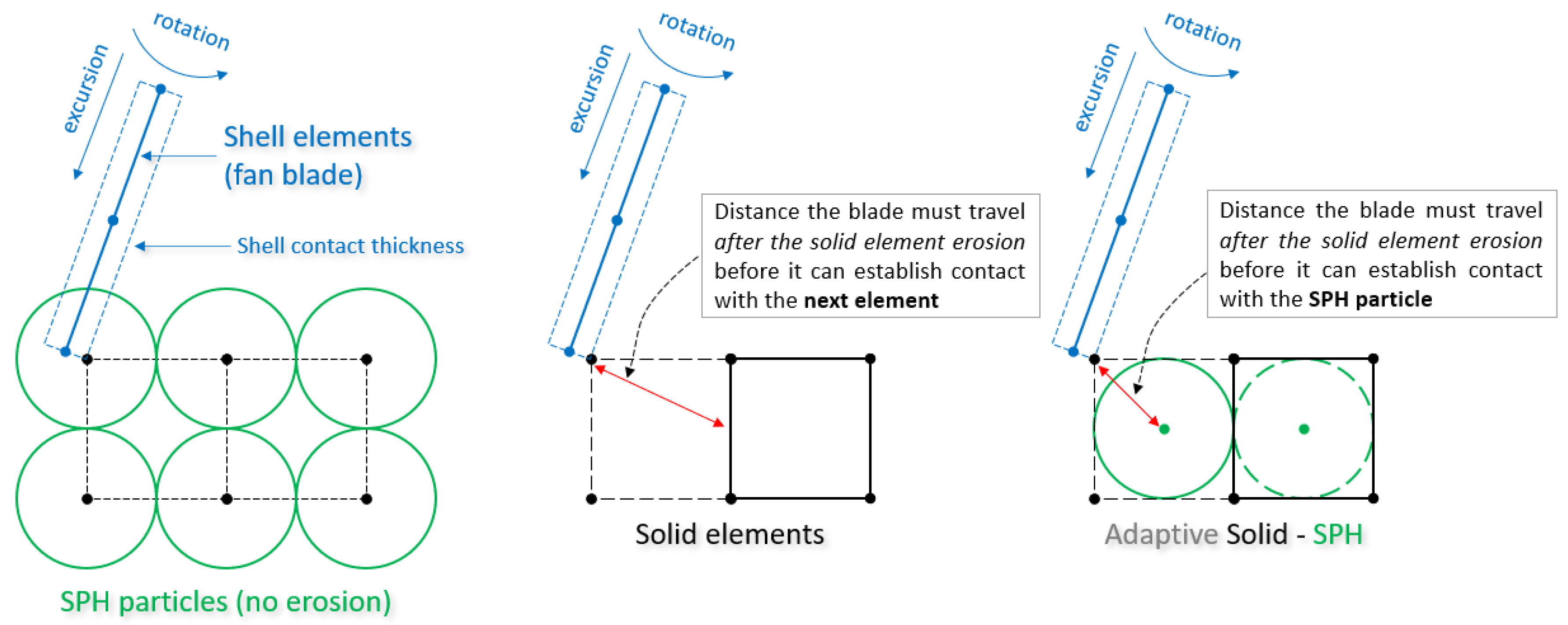
- Smoothed Particles Hydrodynamics (SPH) meshless technique, in which the continuum is modeled as the arbitrary lattice of interacting particles/interpolation points. This method eliminates mesh tangling problems inherent to the Lagrangian finite element method and does not require an erosion algorithm, which often makes it very suitable for high-speed impact problems. The SPH method is, however, known to be more computationally expensive compared to FEM. Therefore, further study was required to decide if the cost–benefit ratio of this method makes it a suitable replacement for FEM in the considered problem.
- Adaptive (Hybrid) FEM/SPH formulation, which permits the adaptive conversion of finite elements to SPH particles at high deformation levels when the traditional finite element method becomes inefficient. In this method, the SPH particles replacing the failed solid Lagrangian elements inherit all the nodal and integration point quantities of the failed solid elements. Potential benefits of this technique, that required evaluation, are the reduced sensitivity to erosion strain compared to the traditional FEM, and a possible reduction in computational time compared to SPH.
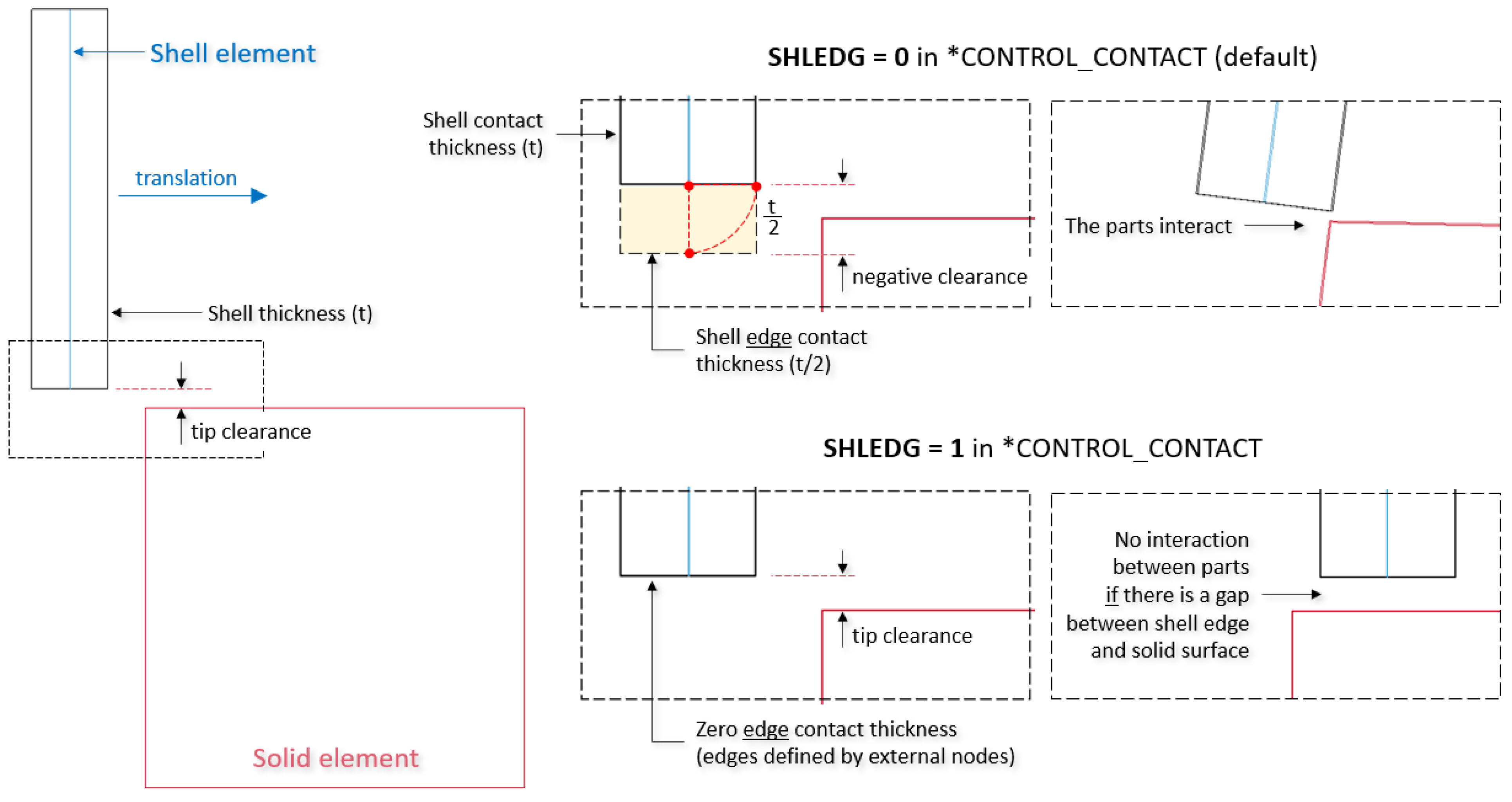
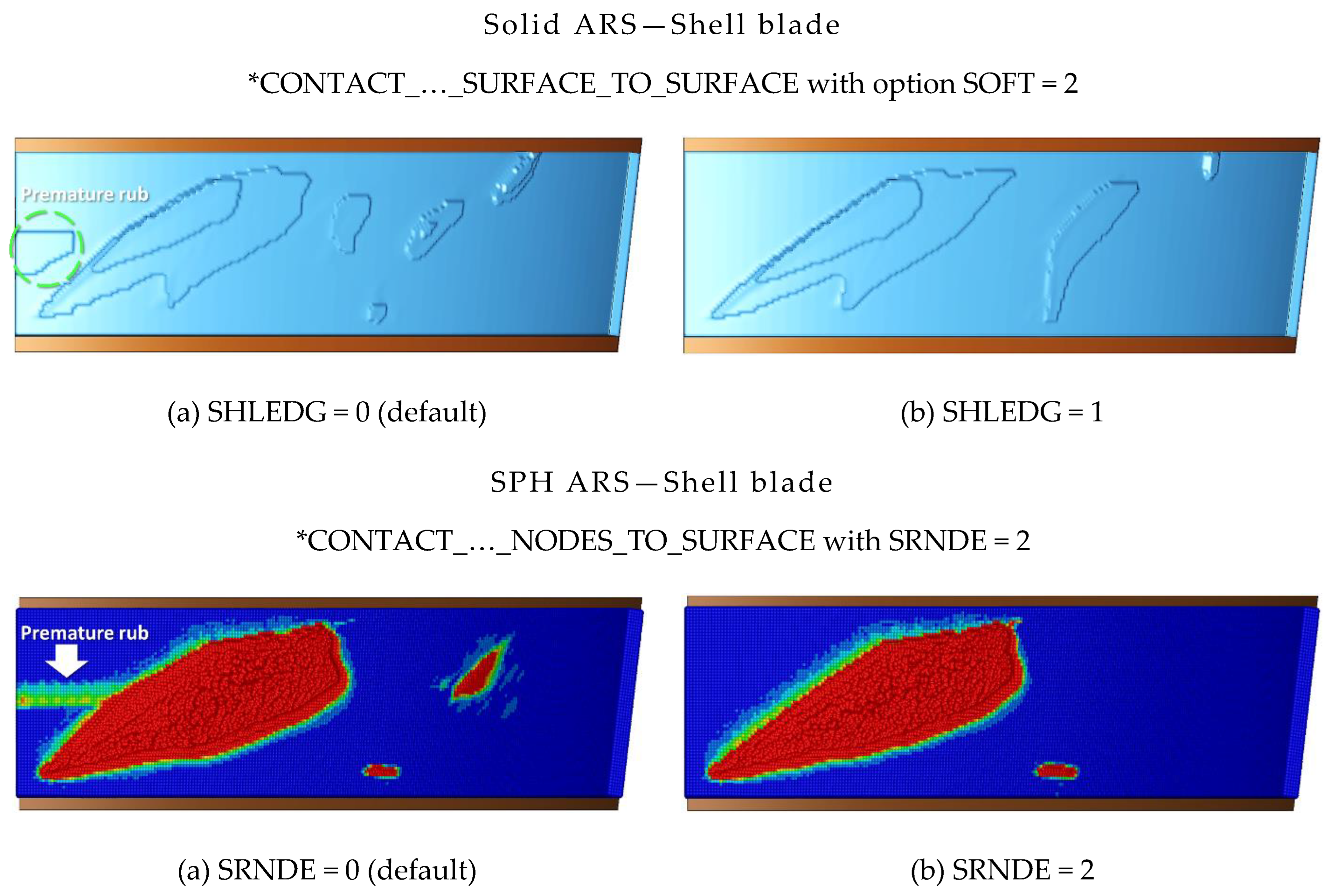
4.3. Contact Modeling
5. Results and Discussion
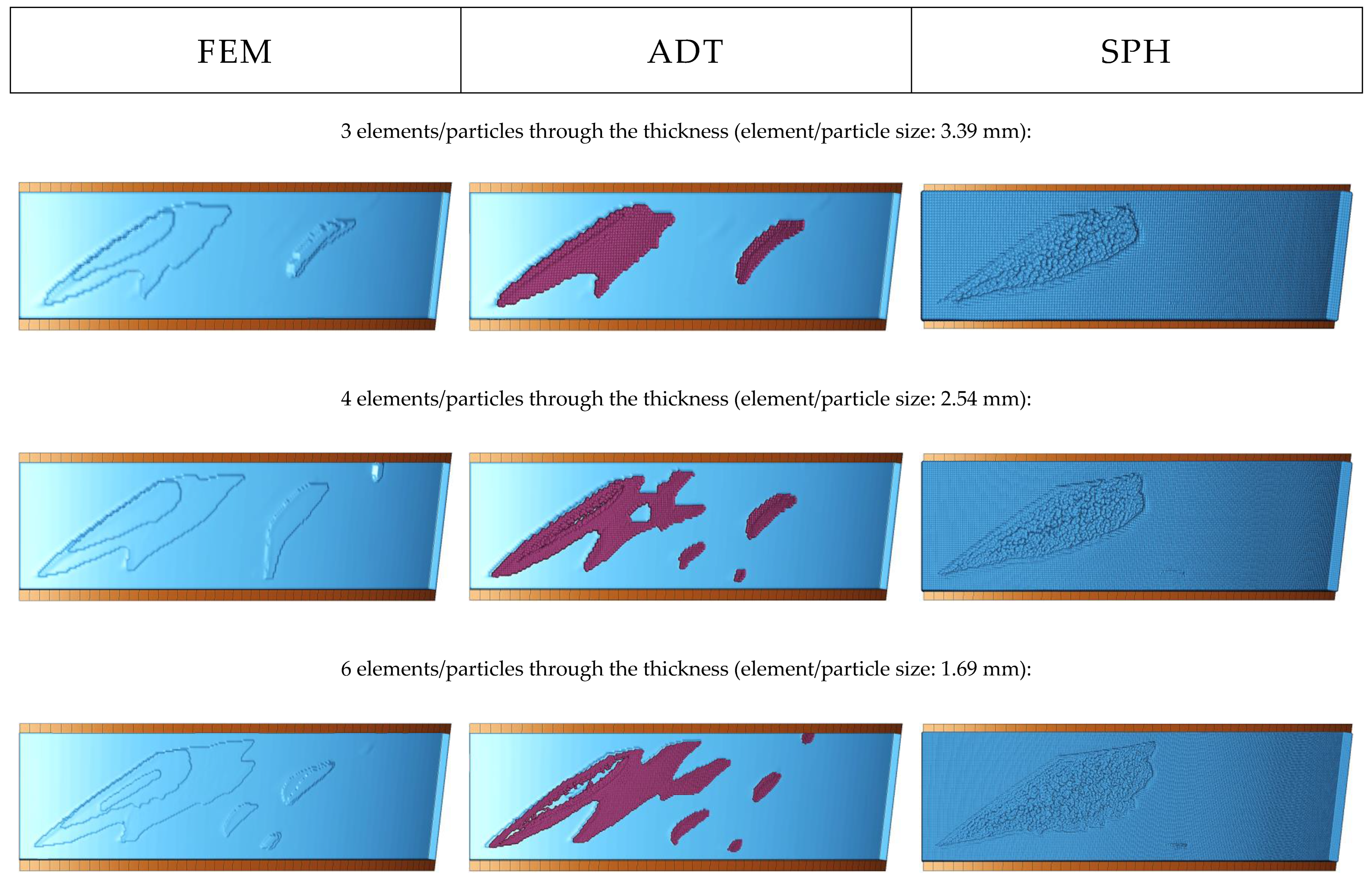
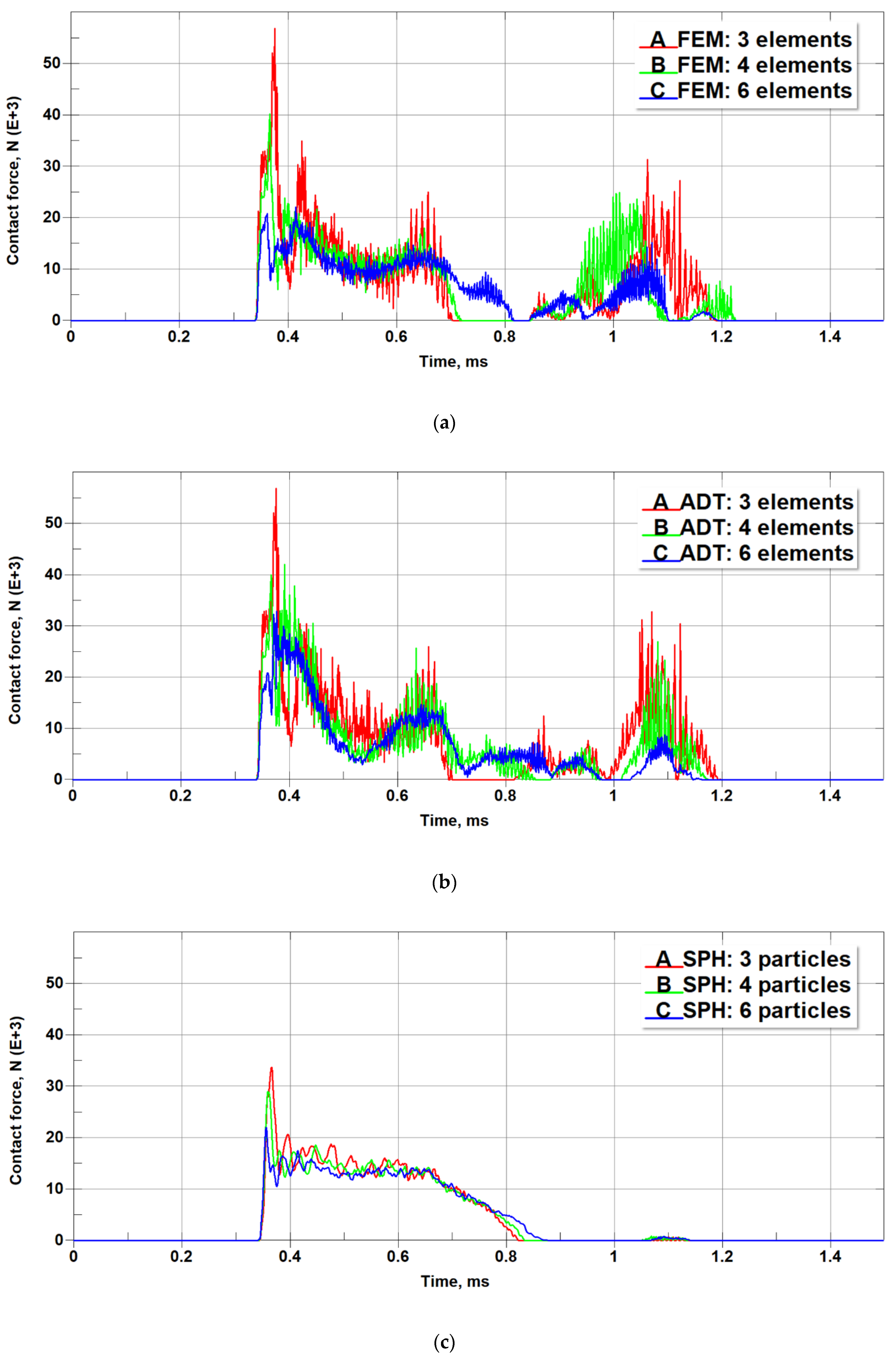
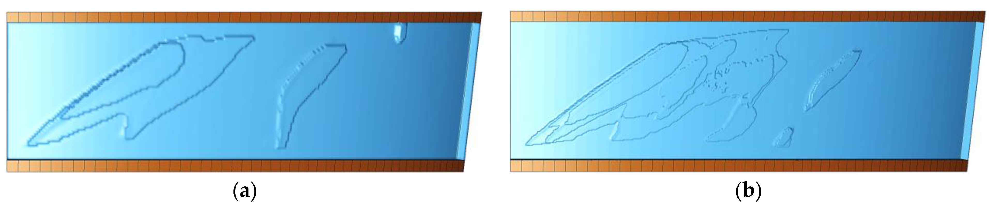
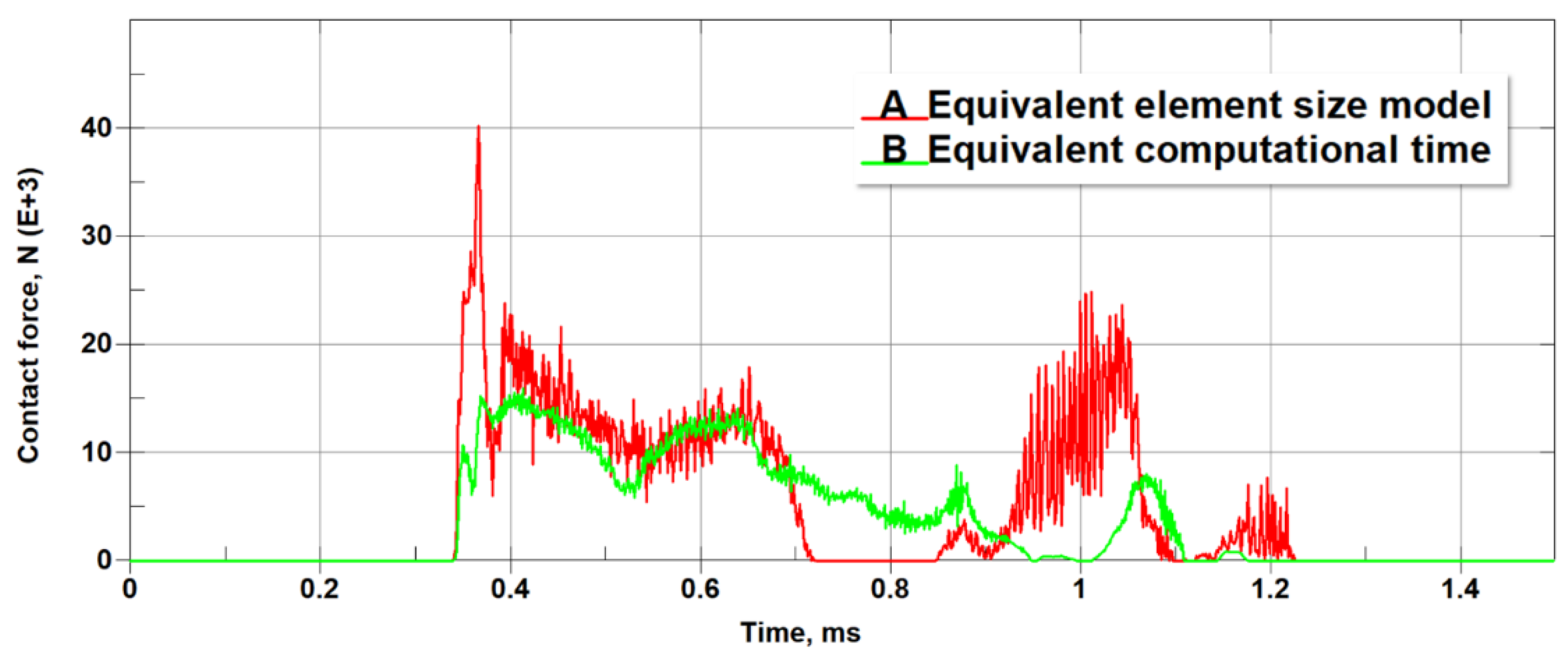
5.1. Mesh Sensitivity
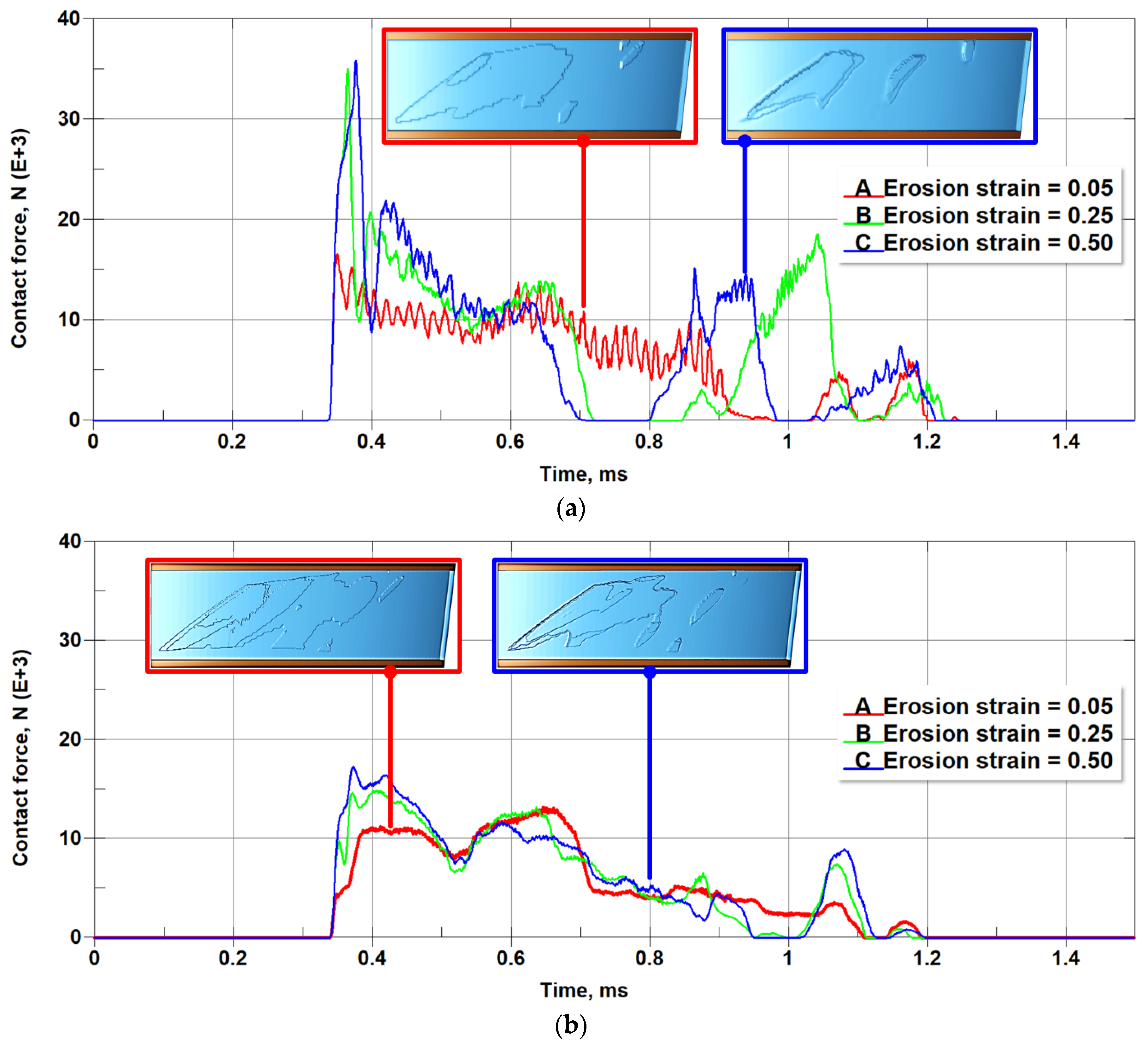
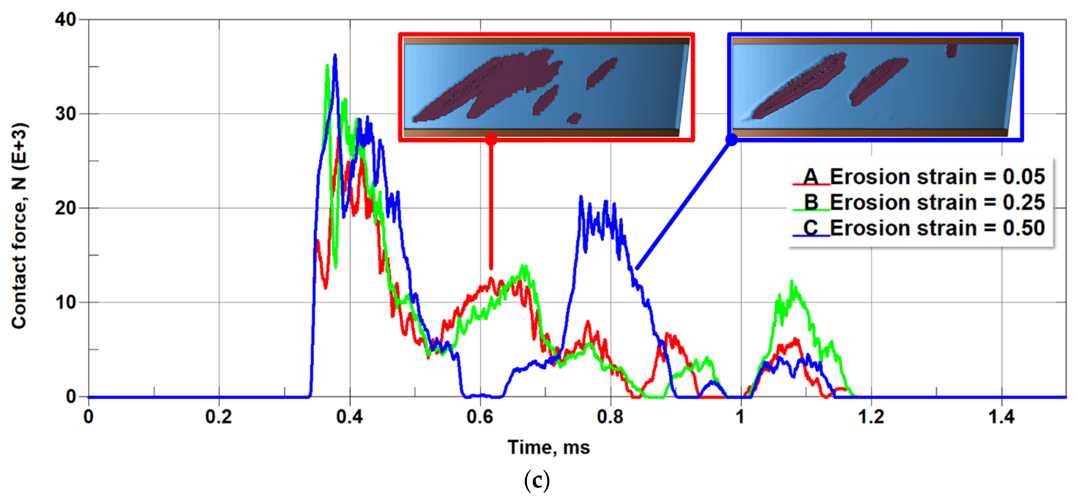
5.2. Sensitivity to Non-Physical Parameters: Element Erosion Strain and Number of Neighboring Particles
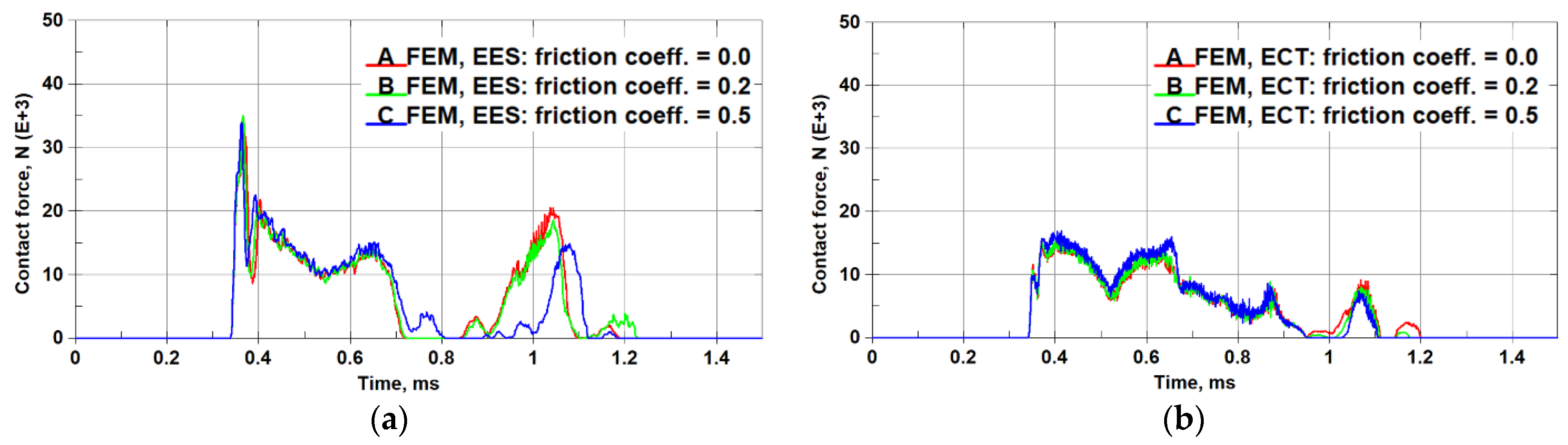
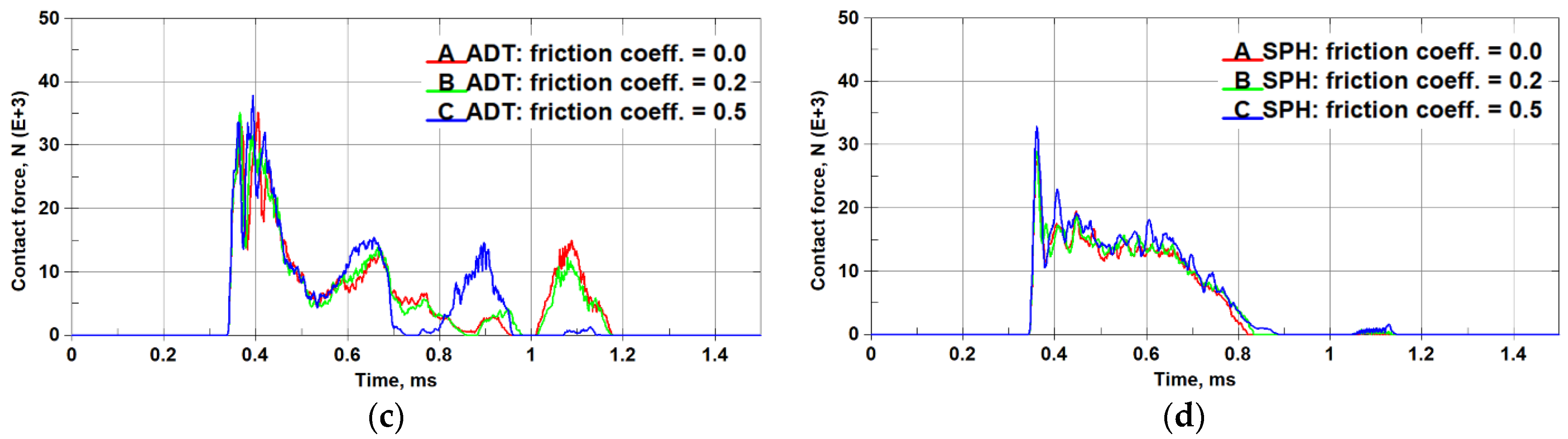
5.3. Sensitivity to Process Parameters: Incursion Depth and Friction Coefficient
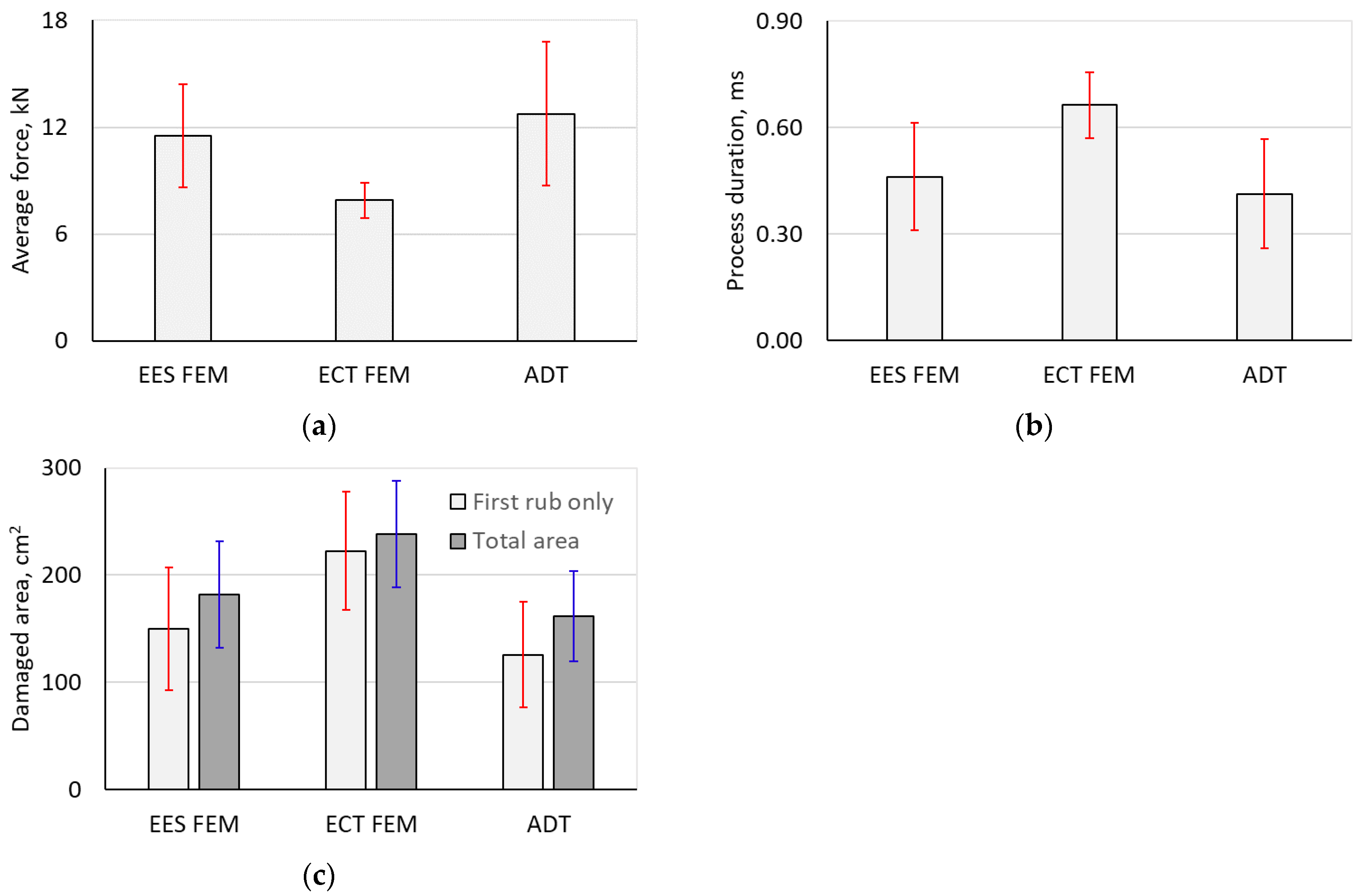
- Large oscillations were noted on the F-t plots of the FEM EES and ADT models (4 elements through the ARS thickness) and, thus, required data filtering. Such effects were not seen with the FEM ECT (10 elements through the thickness) and SPH (4 particles through-the-thickness) models.
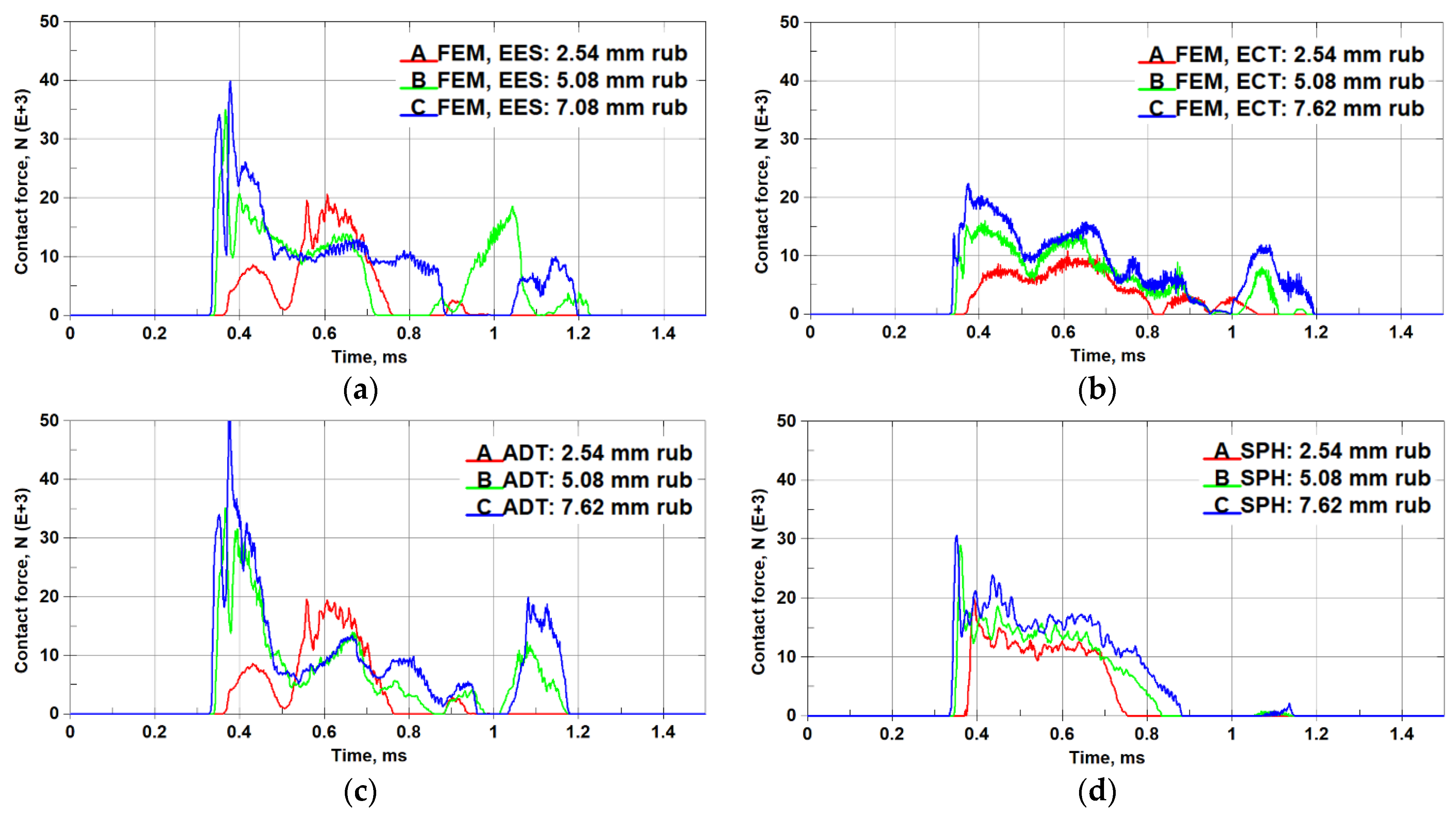
- The FEM (both EES and ECT) and ADT models predicted deep secondary rubs for all three considered incursion depth scenarios. Notably, predictions of the initiation of the secondary rubs, their duration, and force magnitudes are not consistent between the three models (see Figure 20a–c). In contrast, although secondary rubs were also predicted by the SPH model, their magnitudes are negligibly small compared to the primary (first) rub for all the considered rub depths, as can be seen in Figure 20d.
- The shapes/profiles of the F-t curves in the case of the 2.54 mm rub, as predicted by the FEM (both EES and ECT) and ADT models, are notably different from those predicted for the deeper rubs (see Figure 20a–c). In contrast, the SPH model predicted similar “impulse” shapes for all three rub depths (Figure 20d).
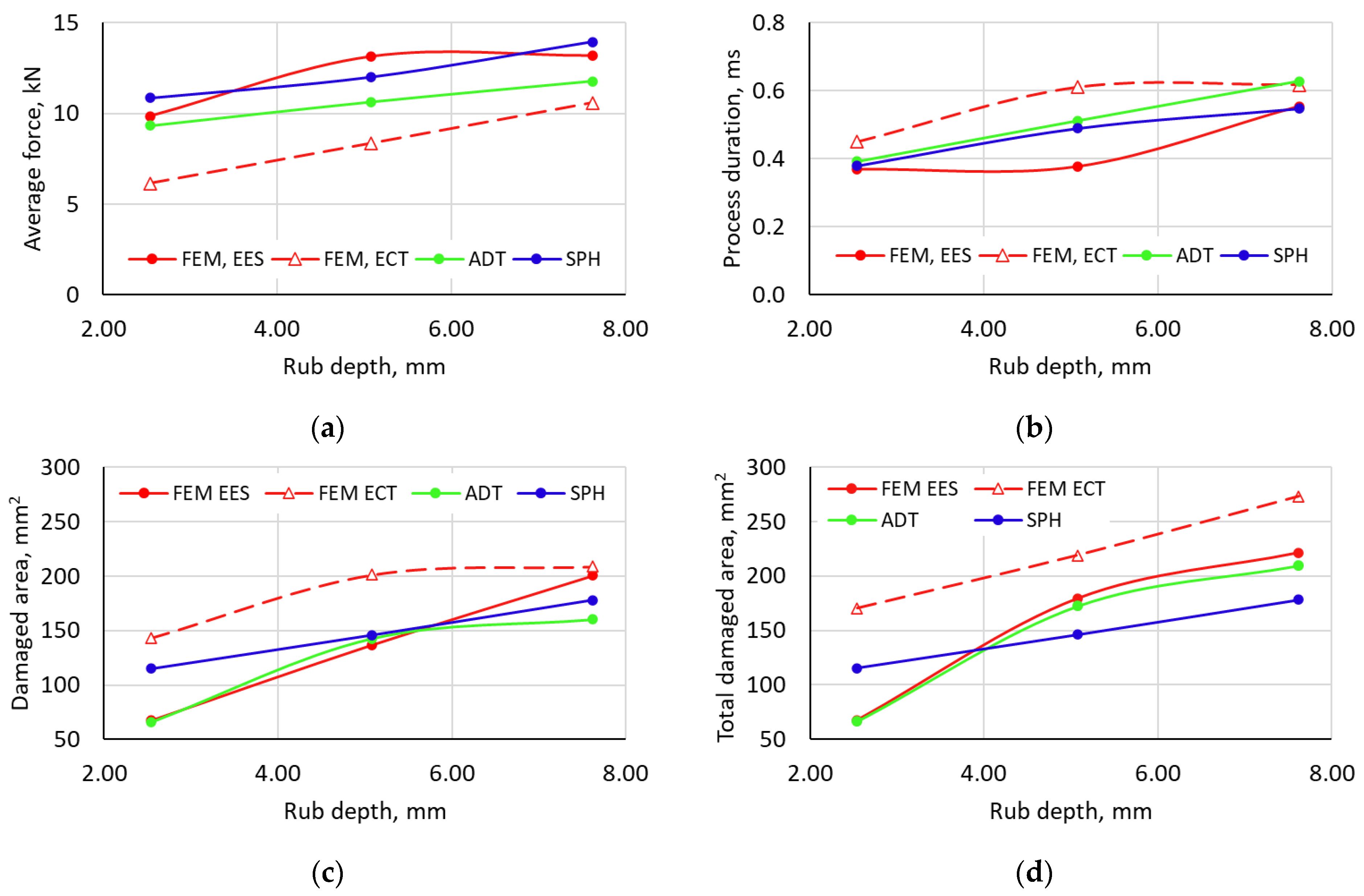
- The SPH model consistently predicts a linear or nearly linear increase in all metrics (average force, process duration, and damaged area) with increase in the rub depth. Such consistency is not seen with all other models.
- With increase in incursion, the FEM ECT model predicts a notably non-linear change to the first rub damage (almost no difference for 5.08 mm and 7.62 mm rubs) and a linear change in the total damaged area. The opposite is true for the FEM EES model.
- The contact force predicted by the FEM ECT model is generally lower compared to the predictions of the other models.
- The predictions of the total damaged area with all incursion depths are notably different for the SPH and the FEM ECT models.
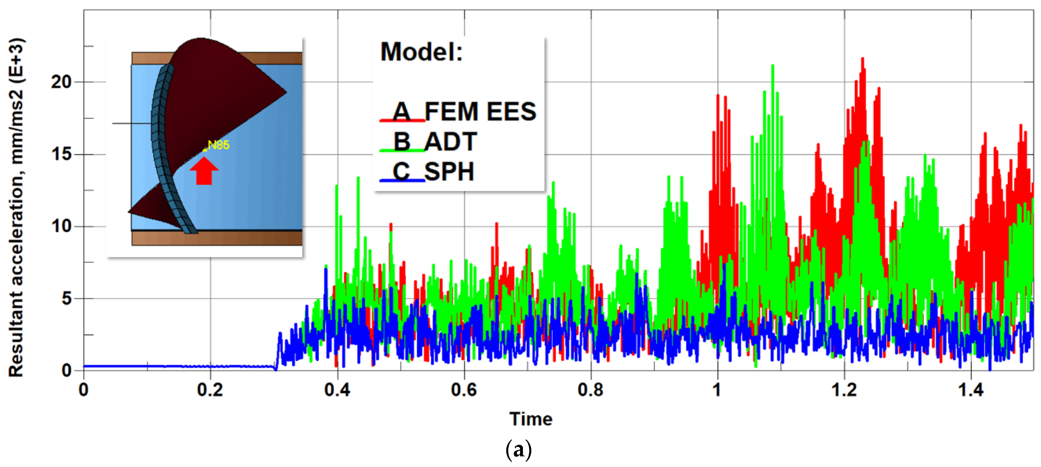
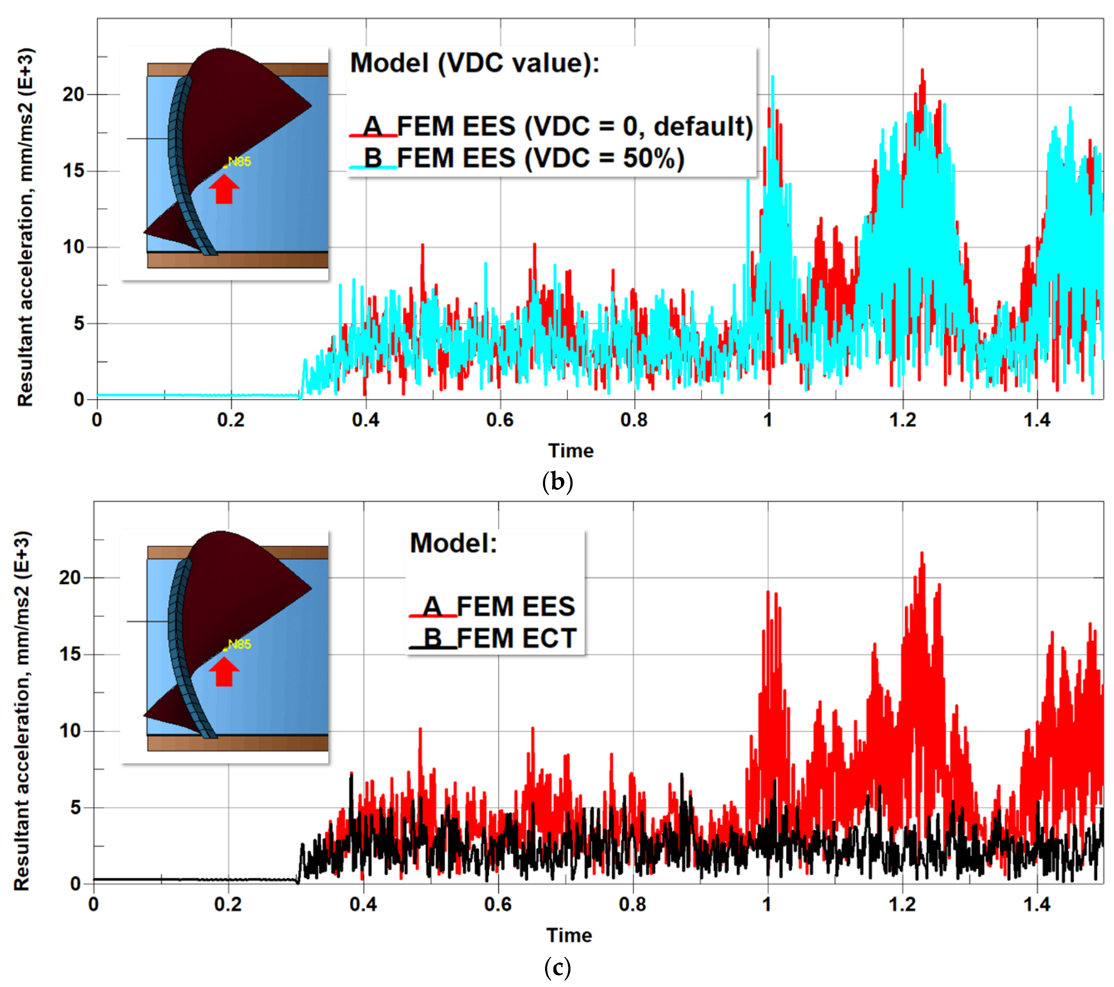
5.4. Additional Remarks
- Excitation of the blade resulting from erosion of finite elements.
- Differences in the contact algorithms used to represent blade–FE ARS and blade–SPH ARS interactions.
6. Conclusions
- Strong mesh sensitivity of the results.
- A strong influence of element erosion strain (a non-physical parameter) on the results.
- Fine meshes are required to reduce spurious oscillations of the blade induced by element erosion, restricting the realization of the computational time benefit.
- Contact definition complexity (number of contact cards required to define interactions between parts of the model) is lower compared to other methods.
- Strong mesh sensitivity of the results.
- A strong influence of element erosion strain (a non-physical parameter) on the re/sults.
- Increasing mesh density to reduce spurious oscillations of the blade may result in an enormous increase in computational time due to the presence of embedded SPH particles.
- No sensitivity to non-physical parameters, such as erosion strain (not used with SPH) and the number of neighboring particles (for models considered in this study).
- Unlike the other models, predicted a consistent trend in change of all the process metrics (rub force, process duration, damaged area) with increase in the rub depth.
- No artificial excitation of the blade was observed.
Funding
Data Availability Statement
Acknowledgments
Conflicts of Interest
References
- Code of Federal Regulations, title 14, part 33. Airworthiness Standards: Aircraft Engines. Available online: https://www.ecfr.gov/current/title-14/part-33 (accessed on 13 September 2023).
- Bin, Y. Blade containment evaluation of civil aircraft engines. Chin. J. Aeronaut. 2013, 26, 9–16. [Google Scholar] [CrossRef]
- Jin, Y. A Review of Research on Bird Impacting on Jet Engines. IOP Conf. Ser. Mater. Sci. Eng. 2018, 326, 012014. [Google Scholar] [CrossRef]
- Cosme, N.; Chevrolet, D.; Bonini, J.; Peseux, B.; Cartraud, P. Prediction of Transient Engine Loads and Damage due to Hollow Fan Blade-off. Rev. Eur. Éléments Finis 2002, 11, 651–666. [Google Scholar] [CrossRef]
- Liu, X.; Raw, J.A. Turbofan Engine Including Improved Fan Blade Lining. U.S. Patent 6,217,277 B1, 5 October 1999. [Google Scholar]
- Hajmrle, K.; Fiala, P.; Chilkowich, A.P.; Shiembob, L.T. Abradable seals for gas turbines and other rotary equipment. In Proceedings of the ASME Turbo Expo 2004: Power for Land, Sea, and Air, Vienna, Austria, 14–17 June 2004. [Google Scholar]
- Department of Transportation, Federal Aviation Administration. Explicit Finite Element Modeling of Multilayer Composite Fabric for Gas Turbine Engine Containment Systems; Final Report. Report No.: AR-08/37; Federal Aviation Administration: Washington, DC, USA, 2009.
- Ivanov, I.; Tabiei, A. Loosely woven fabric model with viscoelastic crimped fibres for ballistic impact simulations. Int. J. Numer. Methods Eng. 2004, 61, 1565–1583. [Google Scholar] [CrossRef]
- Tabiei, A.; Ivanov, I. Computational micro-mechanical model of flexible woven fabric for finite element impact simulation. Int. J. Numer. Methods Eng. 2002, 53, 1259–1276. [Google Scholar] [CrossRef]
- Xu, X.; Li, H.; Feng, G. Influence Factors for Impact Actions and Transient Trajectories of Fan Blades after Fan Blade Out in Typical 2-Shaft High Bypass Ratio Turbofan Engine. J. Therm. Sci. 2022, 31, 96–110. [Google Scholar] [CrossRef]
- Park, C.-K.; Carney, K.; Bois, P.D.; Kan, C.-D.; Cordasco, D. Aluminum 2024-T351 Input Parameters for *MAT_224 in LS-DYNA Part4: Ballistic Impact Simulations of a Titanium 6Al-4V Generic Fan Blade Fragment on an Aluminum 2024 Panel Using *MAT_224 in LS-DYNA; Report Number: DOT/FAA/TC-19/41, P4; Federal Aviation Administration: Washington, DC, USA, 2021. [Google Scholar]
- Legrand, M.; Batailly, A.; Pierre, C. Numerical investigation of abradable coating removal in aircraft engines through plastic constitutive law. J. Comput. Nonlinear Dyn. Am. Soc. Mech. Eng. 2011, 7, 1–21. [Google Scholar] [CrossRef]
- Williams, R.J. Simulation of blade casing interaction phenomena in gas turbines resulting from heavy tip rubs using an implicit time marching method. In Proceedings of the ASME Turbo Expo 2011, GT2011, Vancouver, BC, Canada, 6–10 June 2011. [Google Scholar]
- Salvat, N. Abradable Material Removal in Aircraft Engines: A Time Delay Approach. Master’s Thesis, McGill University, Montreal, QC, Canada, 2011. [Google Scholar]
- Monaghan, J.J. Smoothed Particle Hydrodynamics. Annu. Rev. Astron. Astrophys. 1992, 30, 543–574. [Google Scholar] [CrossRef]
- Xu, J.; Wang, J. Interaction methods for the SPH parts (multiphase flows, solid bodies). In Proceedings of the 13th International LS-DYNA Users Conference, Detroit, MI, USA, 8–10 June 2014. [Google Scholar]
- Department of Transportation, Federal Aviation Administration. Development of a Generic Gas Turbine Engine Fan Blade-out Full-Fan Rig Model; Final Report. Report No.: DOT/FAA/TC-14/43; Federal Aviation Administration: Washington, DC, USA, 2015.
- Husband, J.B. Developing an Efficient FEM Structural Simulation of a Fan Blade off Test in a Turbofan Jet Engine. Ph.D. Thesis, University of Saskatchewan, Saskatoon, SK, Canada, 2007. [Google Scholar]
- Wang, C.; Zhang, D.; Ma, Y.; Liang, Z.; Hong, J. Dynamic behavior of aero-engine rotor with fusing design suffering blade off. Chin. J. Aeronaut. 2017, 30, 918–931. [Google Scholar] [CrossRef]
- Timoshenko, S.P.; Gere, J.M. Theory of Elastic Stability, 2nd ed.; McGraw Hill: New York, NY, USA, 1961. [Google Scholar]
- Wunderlich, W.; Albertin, U. Buckling behaviour of imperfect spherical shells. Int. J. Non-Lin. Mech. 2002, 37, 589–604. [Google Scholar] [CrossRef]
- Ashby, M.F. Metal Foams: A Design Guide; Butterworth-Heinemann: Amsterdam, The Netherlands, 2000. [Google Scholar]
- Cherniaev, A. The use of adaptive FEM-SPH technique in high-velocity impact simulations. In Proceedings of the XI International Conference on Adaptive Modeling and Simulation (ADMOS2023), Gothenburg, Sweden, 19–21 June 2023. [Google Scholar] [CrossRef]


| Interacting Entities | Contact Type and Parameters | Model(s) |
|---|---|---|
| Solid ARS—Shell blade | *CONTACT_ERODING_SURFACE_TO_SURFACE (SOFT = 2) *CONTROL_CONTACT (SHLEDG = 1) | FEM, ADT |
| SPH ARS—Shell blade | *CONTACT_AUTOMATIC_NODES_TO_SURFACE_MPP (GRPABLE =1, SOFT = 0, SRNDE = 2) | SPH |
| SPH ARS—Shell blade/Solid ARS/Shell Tray | *CONTACT_ERODING_NODES_TO_SURFACE_MPP (BT > 0, SOFT = 1) | ADT |
| Shell Tray—Solid ARS (adhesion of matting surfaces) | *CONTACT_TIED_NODES_TO_SURFACE | FEM, ADT |
| Shell Tray—SPH ARS (adhesion of matting surfaces) | *CONTACT_TIED_NODES_TO_SURFACE | SPH |
| Shell Tray—SPH ARS (no particles-through-tray penetration) | *CONTACT_AUTOMATIC_NODES_TO_SURFACE (SOFT = 1) | SPH |
Disclaimer/Publisher’s Note: The statements, opinions and data contained in all publications are solely those of the individual author(s) and contributor(s) and not of MDPI and/or the editor(s). MDPI and/or the editor(s) disclaim responsibility for any injury to people or property resulting from any ideas, methods, instructions or products referred to in the content. |
© 2023 by the author. Licensee MDPI, Basel, Switzerland. This article is an open access article distributed under the terms and conditions of the Creative Commons Attribution (CC BY) license (https://creativecommons.org/licenses/by/4.0/).
Share and Cite
Cherniaev, A. A Comparison of Three Simulation Techniques for Modeling the Fan Blade–Composite Abradable Rub Strip Interaction in Turbofan Engines. J. Compos. Sci. 2023, 7, 389. https://doi.org/10.3390/jcs7090389
Cherniaev A. A Comparison of Three Simulation Techniques for Modeling the Fan Blade–Composite Abradable Rub Strip Interaction in Turbofan Engines. Journal of Composites Science. 2023; 7(9):389. https://doi.org/10.3390/jcs7090389
Chicago/Turabian StyleCherniaev, Aleksandr. 2023. "A Comparison of Three Simulation Techniques for Modeling the Fan Blade–Composite Abradable Rub Strip Interaction in Turbofan Engines" Journal of Composites Science 7, no. 9: 389. https://doi.org/10.3390/jcs7090389