Machine Learning-Based Fatigue Life Prediction of Functionally Graded Materials Using Material Extrusion Technology

Abstract

In this study, the research investigates the prediction of fatigue life for Functionally Graded Materials (FGM) specimens comprising Polylactic acid (PLA) and Thermoplastic Polyurethane (TPU). For this, Machine learning (ML) techniques, including Random Forest (RF), Support Vector Machine (SVM), and Artificial Neural Network (ANN) are utilized. A predictive in-house code is developed for each technique, thereby facilitating the fatigue performance of layered deposited specimens subjected to varying cyclic loadings. In order to verify the effectiveness of the ML technique, a comparative analysis among all is reported based on empirically determined fatigue life obtained values. RF is proven to be the most suitable technique with minimal error percentage in obtained results with optimally synchronized data sets in a minimum time frame. Subsequently, the application of ML in those predictions is reported for future aspects in augmenting the operational efficiency associated with fatigue life prediction.

1. Introduction

Functionally Graded Materials (FGMs) are a material scheme where multi-material properties gradually change within its structure, enabling tailored performance and adaptability to diverse engineering demands in today’s manufacturing [1]. This technology captured considerable attention in various industrial sectors, driven by its unique ability to enhance material performance. The inherent potential of FGMs is not only for advancing material science but also for optimizing the mechanical characteristics of manufactured structures [2]. The development of FGM represents a paradigm shift in materials design, as it allows for precise tailoring of material properties, such as mechanical strength, thermal conductivity, and electrical conductivity, across gradients [3]. This innovative approach offers a remarkable advantage over conventional homogeneous materials, enabling engineers and researchers to design materials with tailored properties that can withstand challenging environments and serve a multitude of applications [4]. FGMs find extensive use in aerospace, automotive, and energy sectors, where the ability to fine-tune material characteristics enables the creation of lightweight, durable, and high-performance components. Additionally, in applications where thermal management is crucial, FGMs have shown promise in efficiently dissipating heat, making them valuable in the development of next-generation electronics and thermal barrier coatings [5]. FGM is found effective for reducing stress concentration and is widely used in aerospace [6].

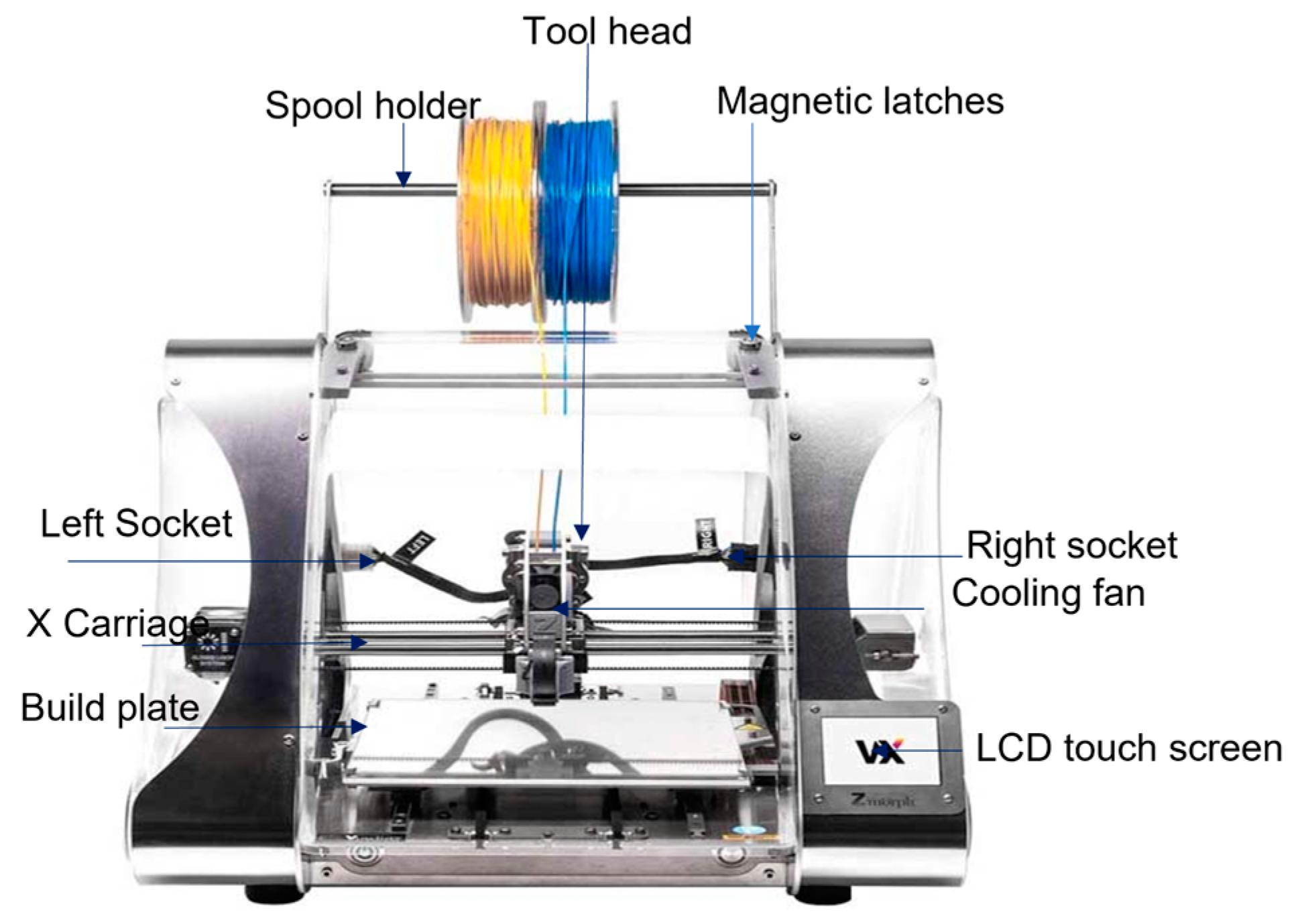
Polymeric FGMs encompass a category of substances characterized by unique compositions and properties that progressively transition throughout their volume. Notably, the fabrication process involves the utilization of additive manufacturing (AM) techniques recognized as Material Extrusion (MEX), alternatively referred to as multi-material additive manufacturing (MMAM) [7]. Unlike traditional homogeneous materials, FGMs offer tailored variations in characteristics such as mechanical strength, thermal conductivity, and stiffness. This engineered gradient imparts FGMs with enhanced adaptability to diverse engineering scenarios, making them particularly relevant in applications where material performance demands are multifaceted [8]. In engineering, FGMs hold significant promise due to their potential to address challenges that conventional materials might struggle to overcome. By seamlessly blending different polymers or incorporating fillers with varying properties, FGMs can be tailored to meet specific requirements within a single structure, as shown in Figure 1. This strategic customization allows FGMs to optimize mechanical responses, reduce stress concentrations [9], and enhance overall durability [10]. As a result, FGMs find utility across a spectrum of fields, including aerospace, automotive, biomedical devices, and more, where precise material adaptation can lead to superior performance and extended product lifecycles [11]. MMAM has engrossed numerous researchers due to its inherent advantages. MMAM facilitates the fabrication of parts encompassing diverse materials in a single manufacturing process, wherein these materials can exhibit distinct chemical, physical, mechanical, and electrical properties [12]. In the last twenty years, AM has emerged as a pivotal technology within the manufacturing industry. AM technologies have revolutionized traditional manufacturing methods by offering several significant advantages. Compared to conventional approaches, AM eliminates the requirement for extensive tooling [13], resulting in cost and time savings [10]. Additionally, AM provides unparalleled flexibility in design and allows for easy modification of products during the manufacturing process. These capabilities empower manufacturers to rapidly iterate and customize designs, leading to improved efficiency and innovation in the production of various components and products [14]. MMAM encompasses a comprehensive classification comprising seven distinct technologies. These include MEX, vat photopolymerization, powder bed fusion, material jetting, direct energy deposition, sheet lamination, binder jetting, and hybrid additive manufacturing [15]. Each technology offers unique capabilities and characteristics, contributing to the versatility and potential of MMAM in achieving precise material combinations and complex part geometries. In the MEX process in MMAM, a variety of materials are utilized, including thermoplastics, metal-filled thermoplastics, composites, and more. Figure 1 provides a schematic view depicting the process description of the MEX process in MMAM [16].

The fatigue life prediction of polymers and composite materials has been characterized by significant efforts to enhance accuracy and efficiency. Numerous studies have employed traditional approaches such as stress-life (S-N) curves and strain-life (ε-N) curves [17], adapting these methods to cater to the unique behaviors of polymeric and composite materials. However, while these conventional methods provide valuable insights, they often fall short when dealing with the intricate and heterogeneous nature of FGMs. This limitation has spurred a growing interest in harnessing the power of ML techniques for fatigue life prediction [18]. A similar study conducted by Hassanifard et al. [19] examined the fatigue life of 3D-printed PLA components through the application of various ML techniques, including linear, polynomial, and RF models. The outcomes indicated that, with the exception of linear regression, the proposed methodologies demonstrated superior predictive capabilities at elevated load levels compared to traditional analytical and numerical approaches. Additionally, Kishino et al. [20] have predicted that the fatigue life of polymer film substrates was accomplished using both linear regression and RF techniques. The outcomes emphasized the exceptional accuracy, efficiency, and resilience of the RF model in foreseeing fatigue behavior across diverse loading scenarios. This study contributes significantly to the domain by showcasing the feasibility of ML in forecasting fatigue life for polymer films. These findings hold the potential to influence material design and applications, particularly those necessitating heightened durability. Subsequently, Boiko et al. [21] encompassed the analysis of empirical data obtained from 3D-printed plastic components. Additionally, an ANN was employed to forecast fracture behavior in the samples. Furthermore, the integration of a thermographic camera aimed to enhance the material’s thermal properties. The results showcased the successful development of fracture time prediction through the utilization of artificial intelligence techniques. Later on, Bao et al. This study delved into the evaluation of fatigue life in Selective Laser Melting (SLM) processed metallic components using the SVM methodology [22]. Essential geometric features associated with critical defects were acquired through advanced techniques such as fractography and surface roughness assessment. The acquired data underwent a rigorous training process and subsequent correlation with fatigue life cycles. The outcomes of this investigation demonstrated the capability to predict fatigue life based on defect characteristics, subsequently facilitating lifetime assessment and validation procedures. Finally, Nasiri et al. [23] have reviewed comprehensively and critically assessed a spectrum of methodologies employed for fatigue life prediction in both metallic and non-metallic components. Drawing insights from a meticulous examination of a diverse array of literature sources from esteemed repositories like Scopus and other literature databases, the study meticulously delineates empirical, data-driven, and statistical approaches. The outcomes, meticulously documented, encompass a thorough exposition of limitations, applications, and methodological rationales intrinsic to the utilization of data-driven techniques in the assessment of fatigue properties across domains encompassing 3D printed parts of metallic, non-metallic, and composite. Furthermore, the review expounds upon the fundamental parameters that assume pivotal roles in determining the fatigue life of both metallic and non-metallic constituents, thereby contributing to the scholarly discourse in this domain.

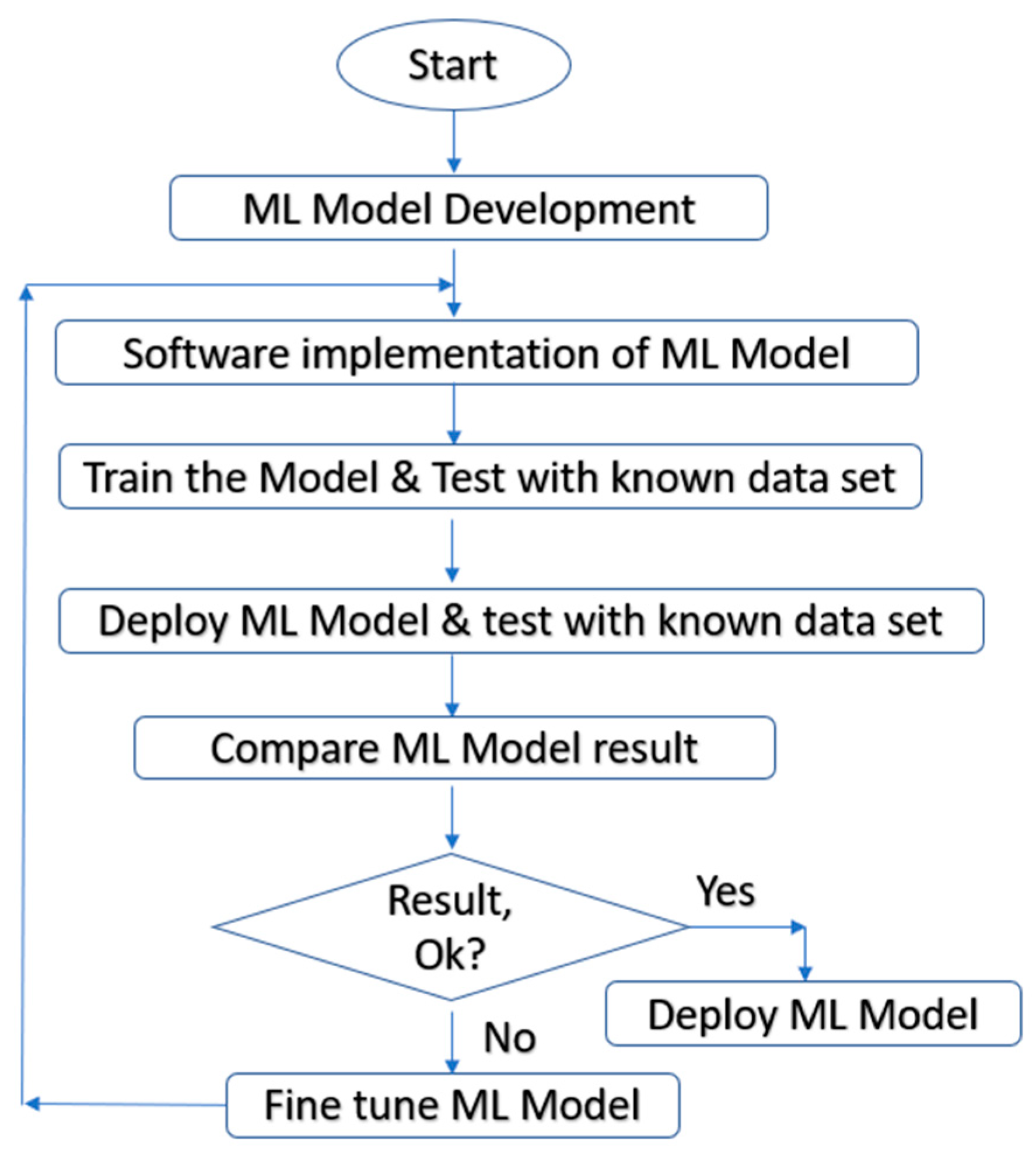
In the pursuit of accurately predicting the fatigue life of polymeric FGMs, a comprehensive implementation of ML techniques has been undertaken, as shown in Figure 2. The model development process commenced with the meticulous formulation of the ML model, tailored to handle the intricacies of FGM materials. Rigorous data preparation and feature engineering were conducted to ensure the dataset’s readiness for the training and testing phases. Subsequently, the software implementation of the ML model was carried out, integrating cutting-edge technologies and frameworks to harness the full potential of predictive analytics [24]. The model underwent extensive training using a diverse dataset comprising known fatigue life values for polymeric FGM materials under varying conditions. Through rigorous testing with the known dataset, the model’s performance and efficacy were thoroughly evaluated, establishing its predictive capabilities. Upon successful validation, the ML model was deployed to facilitate real-world fatigue life predictions for polymeric FGM materials. Using the same known dataset, the model’s predictions were compared against the actual fatigue life values, demonstrating promising results. The model’s accuracy, reliability, and efficiency were assessed to be satisfactory, prompting its deployment for practical applications. Nonetheless, to ensure continuous enhancement, fine-tuning the ML model is an ongoing process, where further adjustments and refinements are made based on additional data and feedback, leading to a continual improvement in fatigue life prediction for polymeric FGM materials. This multidimensional approach to ML implementation stands as a testament to its potential to revolutionize the field of material science and engineering, facilitating safer and more durable structural designs in various industrial domains.

Recent research has shown promising results in employing ML methods such as RF, SVM, and ANN to predict fatigue life in various material systems. These techniques offer the advantage of capturing intricate patterns, non-linear relationships, and complex interactions within datasets, all of which are crucial in deciphering the nuanced fatigue behavior of polymeric FGMs. While existing studies have demonstrated the efficacy of ML in fatigue life prediction, a notable gap in the literature lies in the application of these techniques, specifically to polymeric FGMs. The unique composition and behavior of FGMs present a novel challenge that necessitates dedicated investigation. Thus, this current study aims to bridge this gap by comprehensively exploring the potential of ML methods for accurate fatigue life prediction in polymeric FGMs, thereby contributing to the advancement of both material science and predictive modeling techniques.

2. Materials and Methods

In this study, a ZMorph™ 3D printer, characterized as a single-nozzle dual-material printer, is employed to manufacture multi-material structures. The printer operates based on the MEX technique, facilitating the concurrent extrusion of two distinct materials through a solitary nozzle. This distinctive attribute empowers the fabrication of intricate and utilitarian multi-material entities. An active visual depiction of the ongoing printing process is shown in Figure 3.

The experimental analysis involves the characterization of both tensile and fatigue test samples. This examination aims to explore the response of FGM composites under diverse structural loads. The parameters employed for fabricating the specimens are detailed in

Table 1. Fixed Processing parameters.

Parameters	Values
Nozzle temperature (°C)	210
Bed temperature (°C)	60
Infill density (%)	100
Infill pattern	Line (0/90)
Layer width (mm)	0.35
Layer height (mm)	0.2
Printing speed (mm/s)	15

.

2.1. Specimen Preparation and Fabrication

The specimen conforms to the ASTM standard E606M [25]. The specimen adheres to the ASTM standard E606M [25], as delineated in Figure 4. Concerning the dimensional attributes of the fatigue test specimen, namely length, width, thickness, and curvature radius, these specifications are meticulously set at 135 mm, 20 mm, 5 mm, and 10 mm, respectively. The comprehensive set of specimens investigated in this study is expertly crafted utilizing two distinct filament types: TPU and PLA, each possessing a diameter of 1.75 mm. Notably, the PLA filament exhibits a distinct black pigmentation, while the TPU filament retains its transparency. It is of paramount significance to underscore that all specimens are uniformly manufactured in a horizontal orientation, as clearly exemplified in Figure 4. For a more intricate visual representation of the 3D-printed FGM specimen, as shown in Figure 5. Within this context, Figure 5A provides a comprehensive top-view illustration of the specimen, meticulously fabricated utilizing TPU, resulting in a pristine white appearance. Conversely, Figure 5B offers an alternative perspective of the same specimen, showcasing the utilization of PLA filament in an elegant black. Figure 5C offers a perspicacious vertical view of the specimen, elucidating that one facet of the specimen is composed entirely of 100% TPU in white, while the opposing side embodies 100% PLA in black. Between these two sides, a distinctive FGM layer is deposited, as depicted in Figure 6. Moreover, it aptly serves as an illustrative representation of the intricate multi-material FGM fabrication technique. This visualization offers a lucid insight into the precise process of material blending within the specified A + B zone. The implementation of the Voxlizer slicer underpins this innovative approach, facilitating a highly customizable method for the design of FGMs while adeptly enabling the seamless integration of material gradients.

2.2. Experimental Setup

This investigation involves the assessment of uniaxial fatigue properties of plastics through tensile and fatigue tests conducted using a Testresources 810E4 [26] load frame equipped with 15 KN load cells in accordance with ASTM E606M standard test protocols. Specifically, the experimental setup employed a closed-loop servo-hydraulic machine of the aforementioned model, with control and guidance facilitated through the Newton Testware interface [27]. This interface effectively managed crucial testing variables such as frequency rate, load application, and amplitude. The apparatus incorporates two gripping heads, where the upper head functions as a clamping mechanism, while the lower one acts as a load applicator to the specimen. To maintain the desired stress level, a PID controller is integrated. The experimental configuration is visually depicted in Figure 7.

2.3. Fatigue Testing

An investigation into the mechanical behavior of FGMs polymeric composites under diverse structural loads involved the experimental characterization of tensile and fatigue test samples. The experimental setup encompassed the assessment of various parameters utilized for the fabrication of the specimens. A tension-based fatigue test was executed to ascertain the fatigue life of the FGM under specific operating conditions. The parameters encompassed stress level, stress ratio, and frequency, set at 90% to 40% of the UTS, 0.1, and 3 Hz, respectively. This investigation aims to gain insights into the material’s response when exposed to tension-tension loading scenarios. The recorded outcomes of the FGM specimens, subjected to fixed processing parameters, are summarized in Table 1. Furthermore, the fatigue cycle trend corresponding to the FGM parameters is shown in Figure 8.

2.4. Machine Learning Algorithms

The implementation of ML algorithms in this research study involves the utilization of the K-fold cross-validation technique, a robust validation strategy. In particular, three distinct methodologies, namely RF, SVM, and ANN, have been incorporated. These methods are systematically employed to elucidate patterns and relationships within the data, aiming to extract predictive insights with enhanced generalization capabilities. By integrating these techniques, the study endeavors to discern the underlying complexities of the analyzed dataset, thereby contributing to a comprehensive understanding of the research domain.

2.4.1. K-Fold Cross Validation

K-fold cross-validation is implemented to evaluate the performance and generalizability of the ML models. K-fold cross-validation involves dividing the available dataset into K equally sized folds. The models are trained on K-1 folds and evaluated on the remaining fold. This process is repeated K times, with each fold serving as the test set once. The performance metrics, such as accuracy or mean squared error, are computed for each iteration, and the average performance across all folds is calculated. By employing K-fold cross-validation, the aim is to assess the robustness of the ML models and determine their ability to generalize to unseen data. This technique helps to mitigate issues of overfitting or underfitting by providing a more comprehensive evaluation of the models’ performance across different subsets of the dataset. It also aids in identifying any potential biases or variability in the predictions. The complete dataset was divided into five identical subsets, each accounting for 20% of the total data. Among these, 60% of the data were allocated for training, 20% for testing, and an additional 20% for validation purposes. This division resulted in the creation of five distinct “folds” of data. The arrangement of the data into folds is visually depicted in Figure 9, illustrating the separation of the dataset into five non-overlapping portions. This approach of dividing the data into folds allows for the systematic evaluation of the models’ performance on different subsets, enabling a comprehensive assessment of their generalization capabilities. One experiment was conducted for each fold, allowing for a comprehensive evaluation of the predictive models’ performance. By performing a separate experiment for each fold, the variability in the data were effectively captured, enabling a thorough assessment of the models’ robustness across different subsets of the dataset. This rigorous experimental approach aimed to yield reliable and unbiased results, providing accurate insights into the predictive capabilities of the models.

2.4.2. Random Forest (RF)

As a prominent ensemble learning technique applied in ML and data analysis, it is comprised of multiple decision trees, where each tree is built using a random subset of features and training samples [28]. It combines the predictions of these individual trees to make a final prediction. This technique reduces overfitting and increases the model’s accuracy and robustness [29]. It is also known for its versatility, as it can handle both classification and regression tasks. It is widely used in various fields, including finance, healthcare, and natural language processing, due to its ability to handle large and complex datasets while providing reliable predictions [30]. The RF model was implemented using an ensemble learning technique. Multiple decision trees were constructed, with each tree using a random subset of the training data and a random subset of the input features. The model incorporated a voting mechanism to aggregate the predictions from individual trees and provide the final prediction. Each decision tree was trained using the training dataset, and the splitting criteria, such as Gini impurity or information gain, were employed to determine the best splits at each node. It could capture complex non-linear relationships between the input features and the fatigue life of the polymeric FGM components.

The practice of employing the bootstrap aggregating algorithm is a common and effective approach in the training of RF models. Central to this technique is the process of randomly collecting samples from the dataset, which is formally termed bootstrap resampling [31].

$$T_n=\{\left(A_1,B_1\right)\dots \dots (A_n, B_n)$$

where A is input vector with m variables A = {$A_1, A_2\dots ..A_m\}$ and B is output scalar. The input data are operated to split at every node, and the function $f\left(A T_n\right)$ is established at the end of the training stage [32]. The bootstrap aggregating algorithm selects some samples $f(T_n^1\dots .T_n^z$) and constructs Z prediction and thus, Z outputs

$$B_1^{pre}=f (A, T_n^1) \dots \dots B_z^{pre}=f (A, T_n^z) \mathrm{are} \mathrm{obtained}$$

2.4.3. Support Vector Machines (SVM)

Harnessing robust capabilities for both classification and regression tasks, powerful ML algorithms come into play known as SVM. They work by finding an optimal hyperplane that maximally separates different classes or predicts continuous values. They are based on the concept of support vectors, which are the data points closest to the decision boundary. It can handle both linearly separable and non-linearly separable datasets using kernel functions that map the data into higher-dimensional spaces [31]. These are effective in dealing with high-dimensional data and can handle complex decision boundaries. They have applications in various fields, including image recognition, text classification, and bioinformatics [32]. The model was implemented as a binary classifier to predict the fatigue life of the polymeric FGM components. The aim is to find an optimal hyperplane that separates the data points representing different fatigue life classes. The hyperplane was determined by maximizing the margin, which is the distance between the hyperplane and the closest data points of each class. This model utilized a kernel function, such as linear, polynomial, or radial basis function (RBF), to transform the input features into a higher-dimensional space, enabling better separation of the data points. The SVM model was trained using the training dataset, and the model parameters were optimized to achieve the best classification performance.

In the linear SVM, the aim is to find a hyperplane that best separates two classes. The optimization problem can be formulated as follows: given a labeled training dataset with a feature vector $x_i$ and corresponding labels $y_i$ where $y_i$ $\in$ {−1,1}, the goal is to find the weight vector $\omega$ and bias term b that define the hyperplane with the maximum margin and correctly classify as many points as possible [33].

The optimization problem can be formulated as:

Minimize: $\frac{1}{2}{‖\omega ‖}^2$

Subject to: $y_i$($\omega \ast x_i$ + b) $\ge$ $1$ for all training samples i.

Here, $‖\omega ‖$ is the Euclidean norm (magnitude) of the weight vector $\omega$ The constraints ensure that data points are correctly classified and lie outside a margin of width $\frac{1}{‖\omega ‖}$.

2.4.4. Artificial Neural Network (ANN)

Emulating the structure and functioning of the human brain, computational models known as ANNs have been developed. They consist of interconnected artificial neurons that process and transmit information. They are widely used in various fields, including ML and pattern recognition, due to their ability to learn from data and make predictions or classifications [34]. These are composed of input, hidden, and output layers, with each neuron receiving inputs, applying weights and activation functions, and passing the output to the next layer [35]. Through a process called training, it adjusts their internal parameters to optimize their performance on a specific task. The model’s ability to handle complex patterns and relationships in data makes it a powerful tool for solving complex problems and making accurate predictions. It was implemented using a deep learning framework, such as TensorFlow or PyTorch. The ANN architecture consisted of multiple layers, including input, hidden, and output layers, with varying numbers of neurons. The input layer was designed to accommodate the relevant features and parameters related to the fatigue behavior of the polymeric FGM components. The hidden layers incorporated activation functions, such as ReLU or sigmoid, to introduce non-linearities and enhance the model’s capacity to capture complex relationships. The output layer represented the predicted fatigue life of the components. The model was trained using a backpropagation algorithm, optimizing the weights and biases to minimize the prediction error between the estimated fatigue life and the actual fatigue life obtained from testing.

3. Results and Discussions

In light of the results obtained from the ML techniques, it becomes evident that their application holds substantial promise for enhancing the fatigue life prediction of polymeric FGMs. The comparison of RF, SVM, and ANN reveals distinct insights into their performance and potential utility. Collectively, these ML methods, coupled with their interpretability, hold significant potential for refining design strategies and advancing the durability assessment of polymeric FGMs in diverse engineering applications. The RF model 1 presented here is used to predict fatigue cycles in a dataset. The data are divided into five folds using the K-fold cross-validation technique, with k = 5. In this approach, the dataset is split into five subsets. This process is repeated three times, ensuring that each subset is used as a validation set exactly once. The first three folds represent the training data (actual data), and the fourth fold is utilized as the testing data for the model. Finally, the fifth fold is used for validation purposes, providing a comprehensive assessment of the model’s performance, as shown in Figure 10. Comparing the training RMSE (Root mean squared error) to the testing RMSE provides insights into the model’s generalization ability. In this case, the testing RMSE of 2696.13 is lower than the training RMSE of 3580.32, which indicates that the model is performing better on unseen data than on the data it was trained on. This suggests that the model is capable of generalizing well to new instances, avoiding overfitting, and making accurate predictions on data it has not encountered during training. The model shows promising predictive capabilities and reasonable accuracy in estimating fatigue cycles.

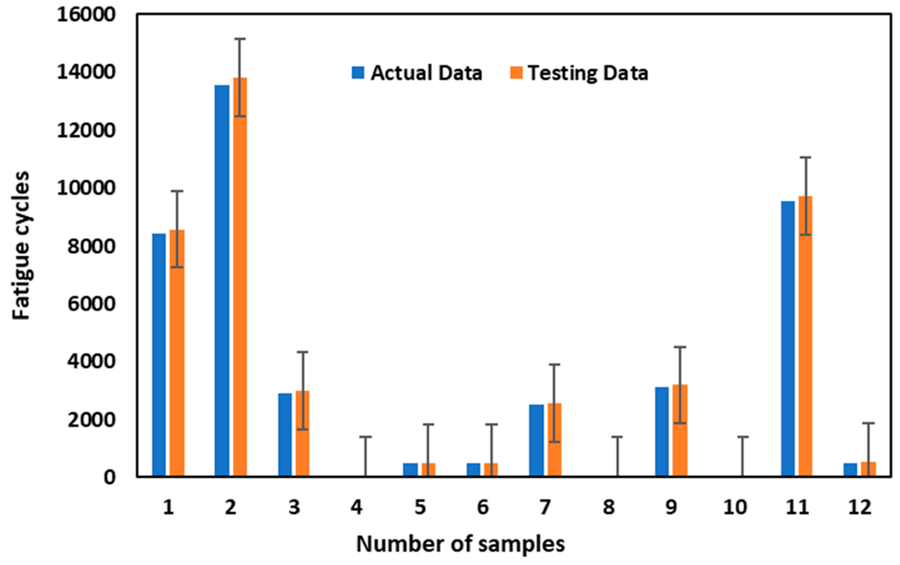
By comparing the results between the training data and test data, the predicted fatigue cycles closely match the actual fatigue cycles for both datasets. In all instances, the predicted values are very similar to the actual values, with minimal discrepancies, as shown in Figure 11. However, this suggests that the model is performing well and generalizing effectively to new, unseen data. Additionally, the predicted fatigue cycles for the test data are almost identical to the actual fatigue cycles, indicating that the model has successfully learned the underlying patterns from the training data and can make accurate predictions for new instances. The testing RMSE of 676.59 represents the average magnitude of the prediction errors made by the model when tested on unseen data (validation data). A lower testing RMSE signifies that the model can generalize effectively to new, unseen instances. The testing RMSE value of 676.59 indicates that, on average, the model’s predictions on the testing data have an error of approximately 676.58 units of the target variable (fatigue cycles).

The RF model 2 presented here is used to predict fatigue cycles in a dataset. For several test data instances, both models provide identical predictions, precisely matching the actual fatigue cycles. These instances include instances 1, 2, 3, 4, 5, 6, 7, 8, 9, 10, and 11 as shown in Figure 12. This alignment indicates a consistent predictive performance by both models for these instances. The comparison between Model 1 and Model 2 reveals that both models demonstrate the ability to accurately predict fatigue cycles for some test data instances. However, there are notable discrepancies in their predictions for several instances.

These differences may arise due to variations in the model architectures, hyperparameters, or the size and composition of their respective training datasets. Model 1 and Model 2 might also incorporate different feature representations, which can impact their predictive capabilities. Moreover, the random nature of the RF algorithm can lead to different outcomes when the models are trained on the same data. It is essential to evaluate both models’ performances on larger datasets and conduct further analysis to determine which model performs better in real-world scenarios and which model’s predictions are more consistent and reliable. Actual data and validation data are shown in Figure 13.

In conclusion, both Model 1 and Model 2 exhibit promising predictive capabilities, showcasing their ability to accurately predict fatigue cycles for the given data. While the models perform admirably, there are some minor variations in their predictions. However, it is important to note that these discrepancies are relatively small, and both models display reliable and consistent performance overall. Further fine-tuning and validation on larger datasets can be undertaken to identify potential areas for improvement and select the most suitable model for specific applications.

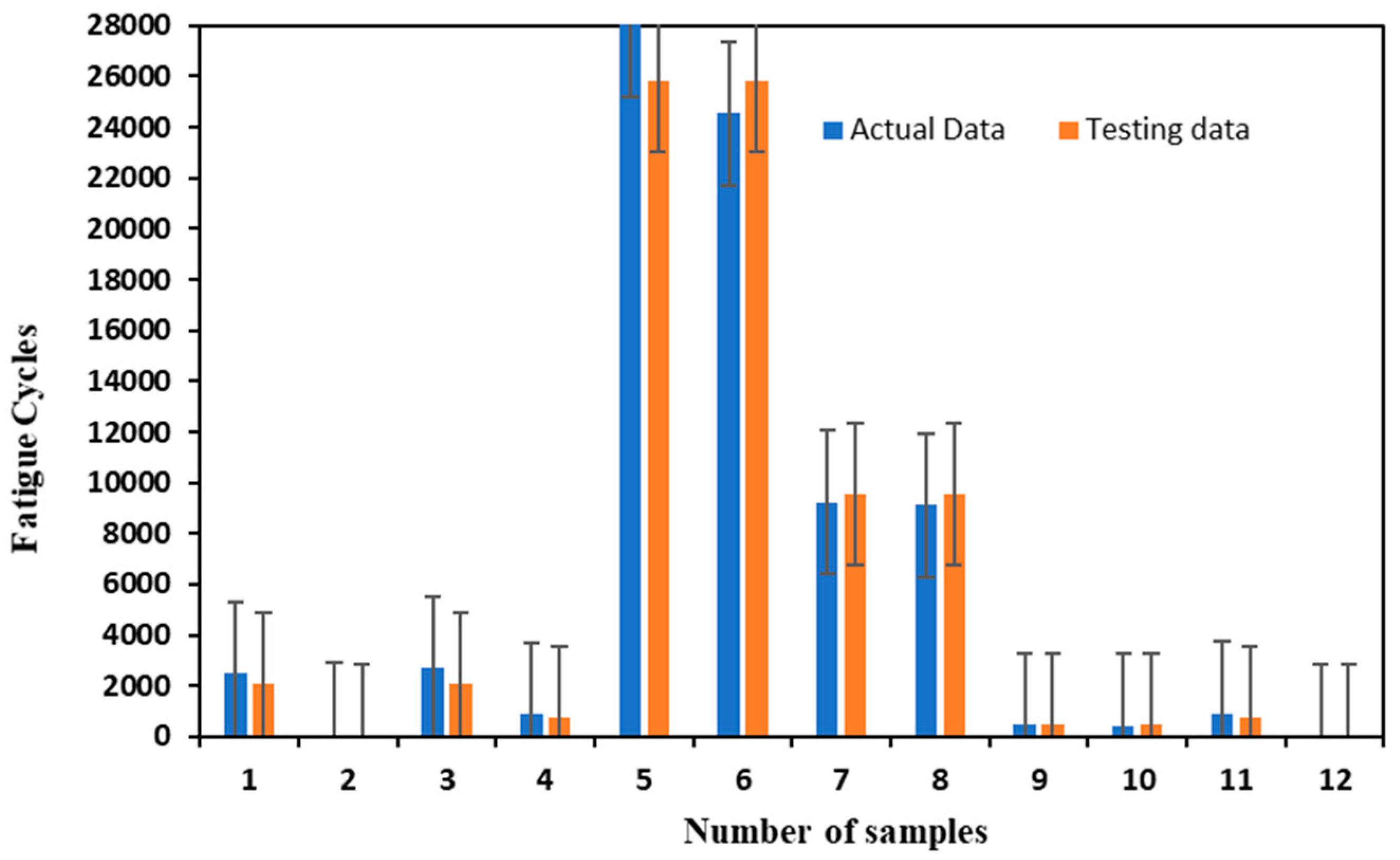
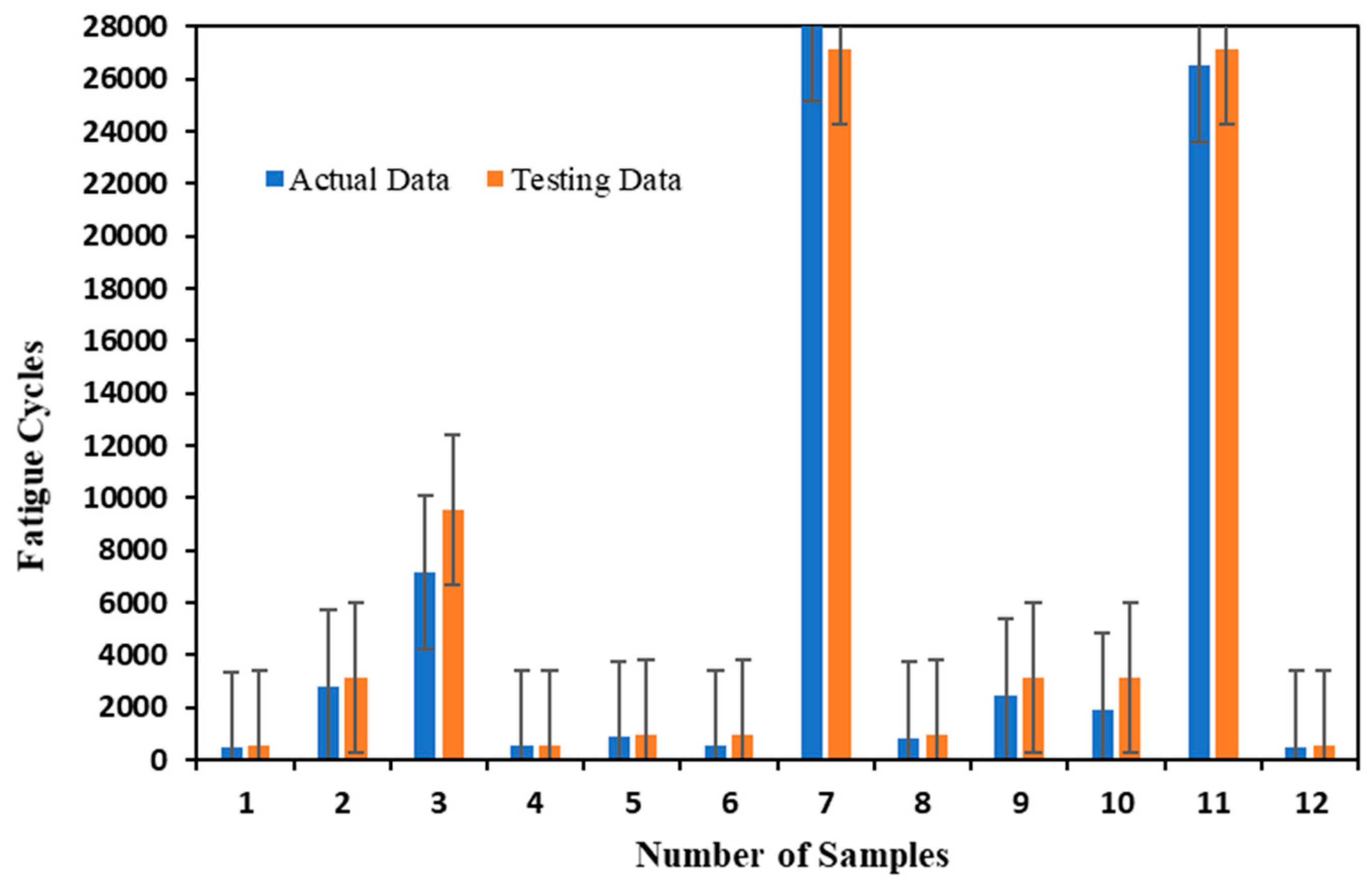
RF model 3 has made predictions on the testing data, and the comparison shows how well the model aligns with the actual fatigue cycle values: For instances 1, 4, 5, and 6, the predicted fatigue cycles are very close to the actual values, indicating accurate predictions for these instances. Instances 2, 9, and 11 show minor variations between the predicted and actual fatigue cycles, suggesting acceptable performance with relatively small prediction errors. Whereas Instances 3, 7, and 12 exhibit more significant differences between the predicted and actual fatigue cycles, indicating potential challenges for the model in accurately capturing the underlying patterns in these cases. Instances 8 and 10 demonstrate moderate discrepancies, indicating a mixed performance where some predictions are close to the actual values while others deviate to a greater extent, as shown in Figure 14. The training RMSE of 1824.17 is lower than the testing RMSE of 2697.38, which is expected and suggests that the model is performing better on the data it was trained on compared to new, unseen data. This indicates that the model has learned from the training data and can make reasonably accurate predictions on that data.

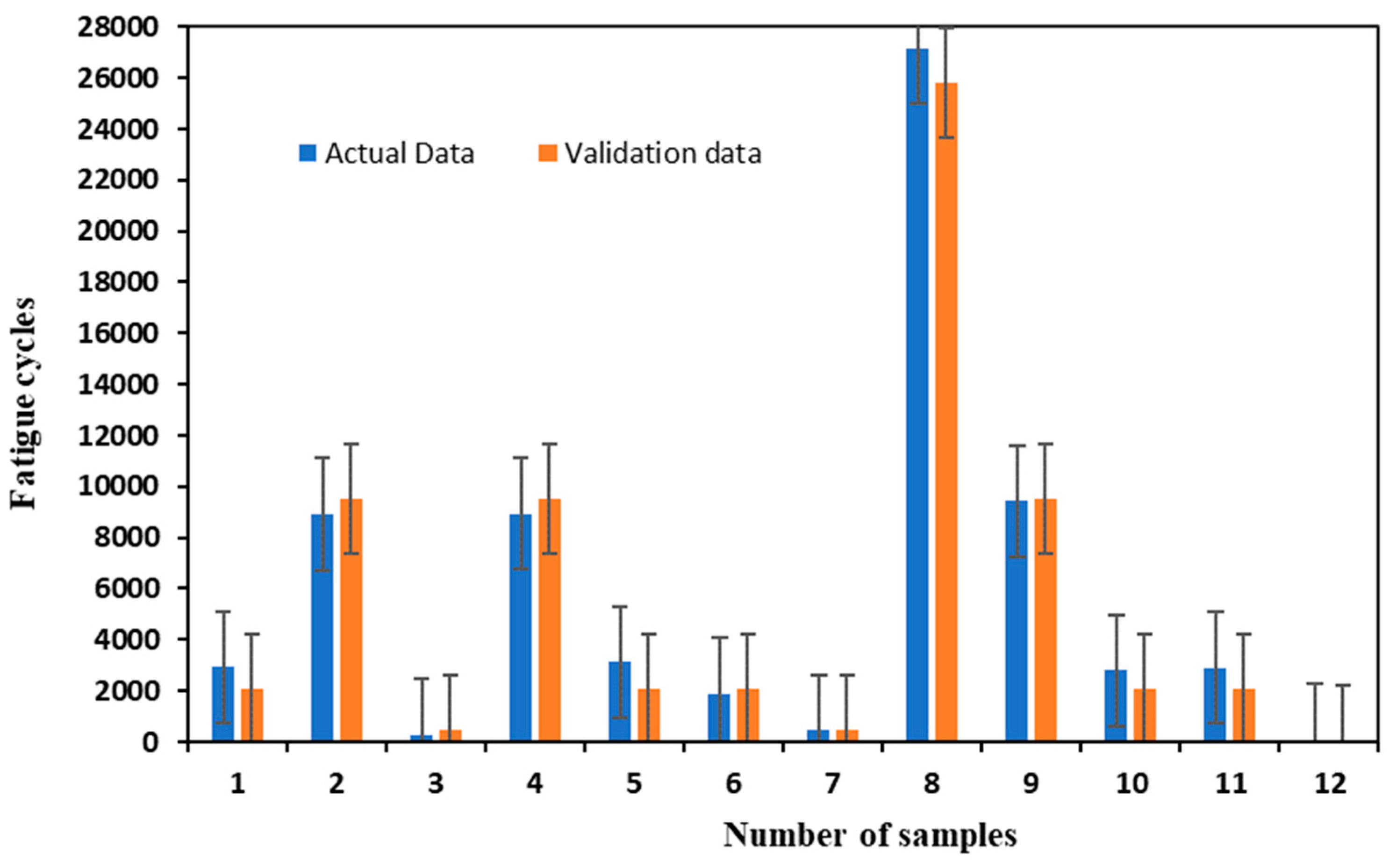
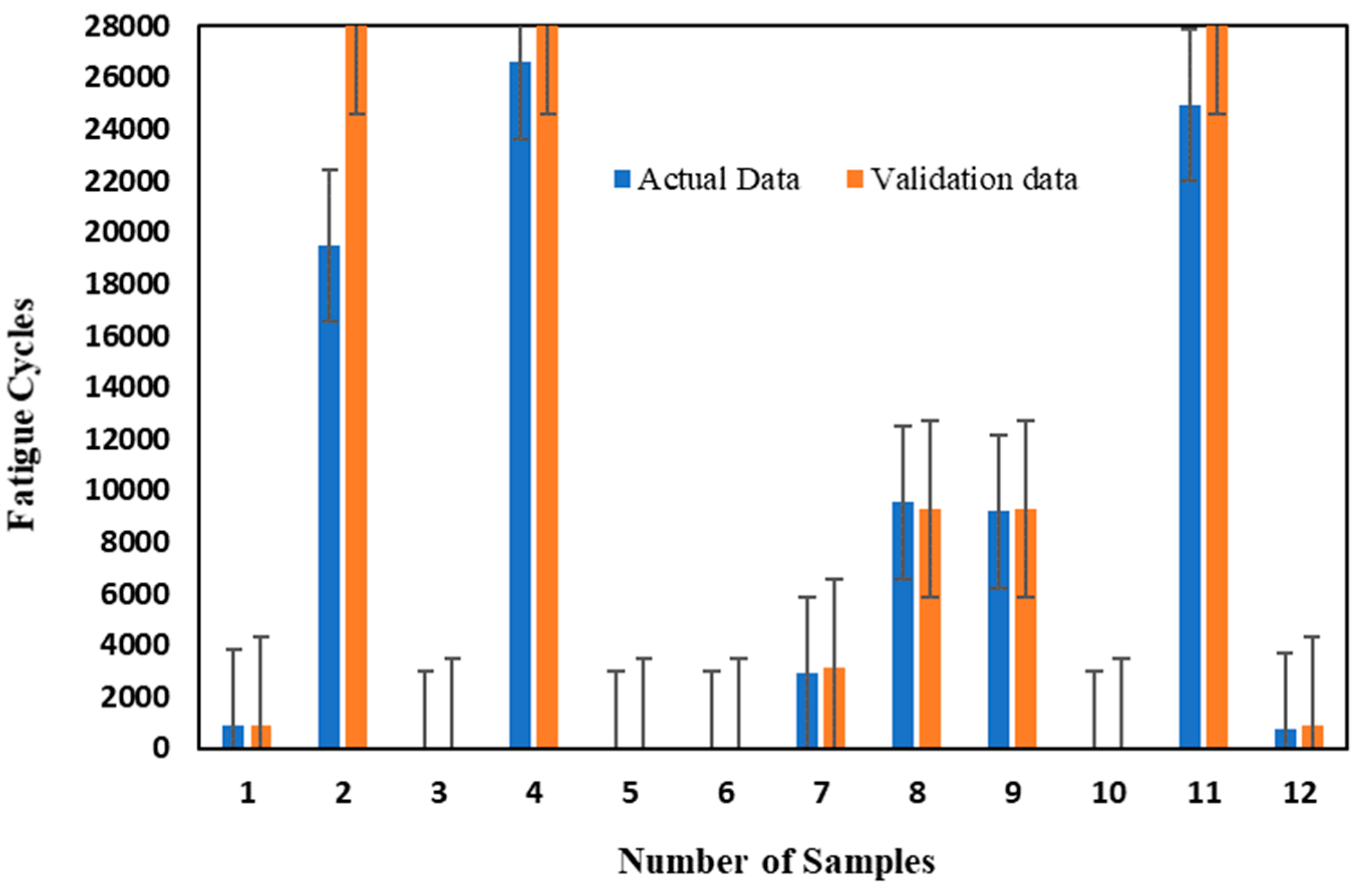
By examining the predicted values from RF model 3 on the validation data, Figure 15 displays how closely the model aligns with the actual fatigue cycle values: Instances 1 and 3 show relatively accurate predictions, with the model closely matching the actual fatigue cycle values similarly Instances 2, 4, 9, 10, 11, and 12 demonstrate accurate predictions as well, indicating good performance by the model on these instances. Whereas instances 5 and 6 reveal minor variations between the predicted and actual fatigue cycles, suggesting acceptable performance with relatively small prediction errors. Eventually, instances 7 and 8 exhibit larger discrepancies between the predicted and actual fatigue cycles. Although the predictions are not far off, there is room for improvement in these cases.

The training RMSE of 760.07 is higher than the testing RMSE of 569.95, which is expected and indicates that the model is performing better on the training data compared to new, unseen testing data. This discrepancy suggests that the model may be experiencing some degree of overfitting. The difference between the training and testing RMSE values suggests that the model’s predictions are more accurate on the testing data compared to the training data. This can be considered a positive sign, as it indicates that the model is able to generalize well to new data.

Models 1, 2, and 3 each demonstrate promising predictive capabilities for fatigue cycle prediction tasks, but they exhibit distinct strengths and weaknesses. Model 1 stands out for its remarkable accuracy and consistency in predicting fatigue cycles, as evidenced by its relatively low RMSE values on both training and testing data. However, it may be limited by potential overfitting, as indicated by a larger difference between training and testing RMSE values. Model 2, on the other hand, showcases comparable predictive performance to Model 1, with slightly higher RMSE values. It appears to generalize well to unseen data, suggesting robustness. Model 3 demonstrates a reasonable ability to predict fatigue cycles with a balance between accuracy and generalization. Its RMSE values for training and testing data are closer compared to the other models, indicating fewer issues with overfitting. To select the most appropriate model, further investigation is required, considering factors such as computational efficiency, interpretability, and the specific requirements of the fatigue cycle prediction application. Overall, each model shows promise, and the choice depends on the specific trade-offs and priorities for the given application.

After examining the predicted values from SVC model 1 on the testing data, the model aligns with the actual fatigue cycle values: Instances 1, 4, and 12 demonstrate accurate predictions, with the model closely matching the actual fatigue cycle values. These instances highlight the model’s capability to predict fatigue cycles with high accuracy. Instances 2, 9, and 10 reveal minor variations between the predicted and actual fatigue cycles, suggesting acceptable performance with relatively small prediction errors. The model still manages to capture the underlying patterns effectively. Instances 3, 5, 6, 8, and 11 exhibit larger discrepancies between the predicted and actual fatigue cycles. While the predictions are not far off, there is room for improvement in these cases, as the model may struggle with certain patterns. Instance 7 showcases the largest discrepancy, where the model significantly deviates from the actual fatigue cycles. This instance highlights a potential area of improvement for the model to better predict high-stress cycles, as shown in Figure 16. The training RMSE of 873.87 represents the average magnitude of the prediction errors made by the SVC model on the training data. A lower training RMSE suggests that the model has learned to fit the training data relatively well. In this case, the training RMSE indicates that, on average, the model’s predictions on the training data have an error of approximately 873.87 units of the target variable.

The testing RMSE of 1163.45 represents the average magnitude of the prediction errors made by the SVC model when tested on unseen data (testing data). A lower testing RMSE signifies that the model can generalize effectively to new, unseen instances. The testing RMSE value of 1163.45 indicates that, on average, the model’s predictions on the testing data have an error of approximately 1163.45 units of the target variable. Instances 1 and 2 exhibit predictions that closely align with the validation data. This indicates that the model has learned to capture the underlying patterns present in both the training and validation datasets effectively. Instances 3, 8, and 9 showcase predictions that differ slightly between the training and validation data. While the model’s performance is relatively accurate in these cases, it may benefit from further fine-tuning to better account for variations in the validation data. Instances 4, 6, and 7 demonstrate significant discrepancies between the training and validation predictions. These instances highlight potential areas where the model could improve its generalization ability and avoid overfitting the training data. Instances 5, 10, 11, and 12 reveal some challenges in predicting the validation data accurately. The model might need additional optimization to better handle instances with varying patterns or stress cycles, as shown in Figure 17.

The comparison between actual data with the testing data predicted by SVC Model 2 provides valuable insights into the model’s performance and its ability to generalize to unseen instances: Instances 1, 2, 4, and 9 showcase predictions that are relatively close to the actual fatigue cycles. This suggests that the model has learned the underlying patterns well and is capable of making accurate predictions on new, unseen instances. Instances 3, 8, and 12 demonstrate predictions with minor discrepancies from the actual fatigue cycles. Although the model’s performance is relatively good in these cases, further fine-tuning may help to improve the accuracy of these predictions. Instances 5, 11, and 10 exhibit precise predictions where the model successfully captures the correct fatigue cycles. These instances highlight the model’s ability to generalize well, even in instances with relatively low-stress cycles. Instance 6 demonstrates a perfect prediction where the model correctly identifies the actual fatigue cycles. This instance indicates that the model has effectively learned the patterns present in the testing data. Instance 7 showcases a prediction that is slightly lower than the actual fatigue cycles. While it is relatively close, there might be room for improvement in capturing patterns for higher stress cycles, as shown in Figure 18.

This RMSE value of approximately 278.84 indicates that, on average, the model’s predictions on the training data have an error of approximately 278.84 units of the target variable. A lower training RMSE suggests that the model’s predictions are closer to the actual values in the training data. The testing RMSE of approximately 718.06 indicates that, on average, the model’s predictions on the testing data have an error of approximately 718.06 units of the target variable. By comparing the model’s predictions on the validation data, we can assess how well it generalizes to unseen instances: Instances 1, 3, 5, 6, 7, 8, and 10 exhibit predictions that closely align with the validation data. This indicates that the model has learned to capture the underlying patterns present in the validation data effectively. Whereas instances 2, 4, and 11 demonstrate predictions that differ significantly from the validation data. These instances suggest that the model may not generalize as well to certain unseen patterns or stress cycles. Additionally, instances 9 and 12 showcase predictions that are relatively close to the validation data but still have minor discrepancies. These instances may benefit from further fine-tuning to improve accuracy, as shown in Figure 19.

SVC Model 2 shows mixed performance on the validation data, with accurate predictions in several instances and minor discrepancies in others. The model’s ability to generalize effectively to unseen validation data are evident in instances where predictions align closely with actual fatigue cycles. Moreover, SVC Model 3 demonstrates promising predictive capabilities on the testing data, with accurate predictions in several instances and minor discrepancies in others. The model’s ability to generalize effectively to unseen testing data are evident in instances where predictions align closely with actual fatigue cycles, as shown in Figure 20.

Instances 1, 7, and 11 demonstrate predictions that closely align with the testing data. This indicates that the model has learned to capture the underlying patterns present in the testing data effectively. Whereas instances 2, 4, and 10 exhibit predictions that closely match the actual fatigue cycles, showcasing the model’s ability to generalize well to these stress cycles. Additionally, instances 3, 5, 6, 8, and 9 showcase predictions that differ slightly from the actual fatigue cycles. While they are not perfect predictions, the model’s performance is relatively good in these cases, as shown in Figure 21. Eventually, by comparing the model’s predictions on the validation data, it demonstrates how well it generalizes to unseen data: Instances 1, 2, 4, 6, and 9 display predictions that closely align with the validation data. This indicates that the model has learned to capture the underlying patterns present in the validation data effectively. However, instances 5, 8, 10, 11, and 12 exhibit predictions that exactly match the actual fatigue cycles, showcasing the model’s excellent performance in these cases. Eventually, instances 3 and 7 showcase predictions that are close to the actual fatigue cycles but have minor discrepancies. While they are not perfect predictions, the model’s performance is relatively good in these instances, as shown in Figure 21.

SVC Model 3 demonstrates promising predictive capabilities on the validation data, with accurate predictions in several instances and minor discrepancies in others. The model’s ability to generalize effectively to unseen validation data are evident in instances where predictions align closely with actual fatigue cycles. Among the three models, Model 3 demonstrates the best overall performance. It has the lowest RMSE values for both training and testing data, indicating that it generalizes well to unseen instances while accurately capturing patterns in the training data. Model 1 and Model 2 show weaknesses in their respective areas, with Model 1 possibly underfitting and Model 2 potentially overfitting. For practical applications, Model 3 would likely be the preferred choice due to its better generalization and prediction accuracy. However, further evaluation and refinement might be needed to achieve even better predictive capabilities. It’s important to note that model performance may vary based on the specific dataset and problem domain, and conducting additional experiments and analyses would provide more robust insights into the model’s performance.

The ANN model architecture consists of a single hidden layer with ten neurons, utilizing the ‘RELU’ (Rectified Linear Unit) activation function to introduce non-linearity. The output layer contains one neuron. The model is then compiled using the mean squared error (MSE) loss function and the Adamax optimizer with a learning rate of 0.001. The training data are then used to train the model for 200 epochs with a batch size of 50. During the training process, the model updates its parameters to minimize the mean squared error between the predicted outputs and the actual target values. Once training is complete, the model is capable of making predictions on new, unseen data. By feeding the testing data (test) into the trained model, it will generate predicted values for the corresponding instances. These predicted values can be compared with the actual target values to assess the model’s performance on unseen data. If the model has learned meaningful patterns during training, it should provide accurate predictions on the testing data.

The comparison of actual data and testing data instances from the ANN Model demonstrates that the model is making accurate predictions on the unseen data, as shown in Figure 22. The small differences between the actual and predicted fatigue cycles indicate the model’s effectiveness in generalizing to new instances beyond the training data. This suggests that the ANN Model is a promising tool for fatigue cycle prediction tasks, showcasing its potential to be applied to real-world scenarios with confidence in its accuracy. However, it’s essential to continue evaluating the model’s performance on diverse datasets and further fine-tuning the model to enhance its robustness and reliability.

Figure 23 displays the results of the ANN Model, depicting the true labels (actual fatigue cycle values) against the predicted labels (model-generated fatigue cycle values). The close alignment between the true and predicted labels signifies the model’s accuracy and effectiveness in predicting fatigue cycles.

4. Limitations and Future Work

This study significantly advances the prediction of fatigue life for FGM through ML. It is essential to acknowledge certain limitations. These include the relatively limited variability in our dataset, potentially hindering the models’ ability to address the full spectrum of FGM compositions and environmental conditions. Additionally, the interpretability of ML models, particularly ANN, poses challenges, making it imperative to explore model interpretability techniques. The computational demands of complex ML models also merit consideration, and the study predominantly focuses on FGMs produced via MEX.

In terms of future research, several promising directions merit exploration. Firstly, expanding the dataset to encompass a broader range of FGM compositions, loading conditions, and environmental factors could enhance the robustness and generalizability of our ML models. Additionally, the development of model interpretability techniques specific to FGM fatigue prediction would enhance the practical utility of these models. Investigating the application of ML in predicting fatigue life for FGM components produced through diverse manufacturing techniques and considering multiscale modeling to capture the hierarchical structure of FGMs could provide more accurate representations of material behavior. Integrating environmental factors and exploring hybrid models that combine ML with physics-based models like Finite Element Analysis (FEA) represent further avenues for refining and extending fatigue life prediction methodologies for FGM.

5. Conclusions

The present study provides valuable insights into the prediction of fatigue cycles in polymeric FGMs through the utilization of ML techniques. The analysis of RF, SVC, and ANN models reveals distinct trends and performance disparities, leading to significant implications for engineering design and material assessment. By examining the performance metrics and characteristics of each model, a comprehensive understanding emerges regarding their suitability and limitations in the context of predicting fatigue cycles in polymeric FGMs. The results of this investigation have been summarized as follows.

• RF model exhibits superior performance in predicting fatigue cycles of polymeric FGMs compared to SVC and ANN models.
• RF model demonstrates the lowest testing RMSE and showcases strong generalization capabilities to unseen data.
• The lower testing RMSE signifies the RF model’s capacity for accurate fatigue cycle predictions in polymeric FGMs.
• RF model’s ability to minimize overfitting while maintaining excellent prediction accuracy underscores its robustness and reliability.
• RF model’s suitability as a valuable tool for engineers and researchers seeking precise and efficient fatigue cycle predictions in polymeric FGMs.
• There is a need for further research and experimentation to validate these results across diverse datasets and establish the RF model’s superiority in various practical scenarios.

This study effectively addresses the gap by comprehensively exploring ML techniques for accurate fatigue life prediction of FGMs. Its future direction includes microscopic component analysis for failure identification enhancing material behavior understanding.