A Systematic Method for Assessing the Machine Performance of Material Extrusion Printers

Abstract

The performance assessment of additive manufacturing (AM) printers is still a challenge since no dedicated standard exists. This paper proposes a systematic method for evaluating the dimensional and geometrical performance of such machines using the concept of machine performance. The method was applied to an Ultimaker 2+ printer producing parts with polylactic acid (PLA). The X and Y axes of the printer were the most performant and led to narrower potential and real tolerance intervals than the Z axis. The proposed systematic framework can be used to assess the performance of any material extrusion printer and its achievable tolerance intervals.

1. Introduction

According to ISO 52900 [1], the additive manufacturing (AM) process consist in “joining materials to make parts from 3D model data, usually layer upon layer, as opposed to subtractive manufacturing and formative manufacturing methodologies”. This process has been gaining more and more interest in industry since its first commercial use in the 1980s [2]. Indeed, AM processes allow parts with complex shapes and geometrical features to be produced at a low cost, as conventional subtractive processes are not able to produce them without requiring assembly, which entails a higher cost [3]. Moreover, in the context of more sustainable processes, AM promises to reduce bulk material consumption as well as enabling lightweight and topological optimized designs to be produced [3]. Furthermore, some AM processes allow feedstock made from recycled parts to be used [4]. Among the seven families of processes defined by ISO 52900, material extrusion (MEX) will be a game changer in the coming years [5]. Indeed, ceramic and metal parts can be produced via MEX at a more competitive cost compared to the other AM processes such as powder bed fusion (PBF) or directed energy deposition (DED), which rely on more expensive feedstock [6]. Therefore, the present study focused on MEX processes owing to their advantages and potential in the near future.

However, even with their possibilities compared with those of subtractive processes, the AM processes suffer from

• Low build rates: from about 0.5 ${\mathrm{cm}}^3/\min$ (for PBF and MEX) to 17 ${\mathrm{cm}}^3/\min$ (for DED) [3,7] (except for large-scale MEX);
• Variable surface finish: arithmetic roughness (Ra) from 0.7 µm to 38 µm for material extrusion printers [8] (depending on the type of measured surface);
• The need for postprocesses to enhance surface topography or to remove the support structures required got the build [2];
• A one or two orders of magnitude higher specific energy consumption than conventional subtractive processes such as machining [9]. The specific energy Cconsumption (SEC) for AM processes ranges from 85 kJ/cm³ for MEX up to 4580 kJ/cm³ for PBF [9], while conventional processes such as milling have a lower SEC of 5 kJ/cm³ to 14 kJ/cm³ [10], depending on the cutting conditions and material milled.

Another major drawback of AM processes is the lack of standards due to their relative youth compared to conventional processes, such as machining, for example, [11,12]. This has hampered the widespread use of AM in industry (especially in critical sectors, such as in the biomedical, aeronautical, military, automotive, and energy sectors) [11]. Indeed, even with the creation of two technical committees (ASTM F42 and ISO/TC 261) [3], there is still lack of data in some areas, such as the methods to assess the dimensional and geometrical performance of AM printers [13]. In the design stage, the resulting tolerance intervals (TIs) allow the fitting between parts to be foreseen as well as the machining stock allowance to be determined. As hybrid machines combining additive and subtractive processes are developing at a high pace, these tolerances and stock allowances are of prime interest [14]. As stated by Dantan et al. [15], achieving predictable and repeatable shapes is critical, while this remains a technological limitation, reducing the impact of AM in various sectors. Reducing the process variability as well as the sensitivity to process variations is then of prime interest to achieve these goals. Another example of an AM application where the clearance between parts is essential to know and anticipate can be found in the manufacturing of nonassembly mechanisms via AM [16,17]. Producing functional mechanisms in a single step without requiring an assembly phase is made possible by the AM process and allows cost and time savings [16]. However, despite the increasing interest in these solutions, the AM of nonassembly mechanisms is still in infancy due to the lack of data for the dimensional and geometrical performance of the machine [16].

In the last decade, many authors have developed methods to assess dimensional and geometrical printer accuracies using a part called the Geometrical Benchmark Test Artifact (GBTA) [12]. This part is printed first and then measured, usually with contact measurement means such as coordinate measuring machines (CMMs). The data are then processed and can lead to the determination of the achievable geometrical and dimensional tolerance intervals [18]. Recently, ISO 52902 [19] presented a standard method decomposing a GBTA into several simpler parts focusing on accuracy, resolution, surface texture, and labeling [20]. Nevertheless, as explained by de Pastre et al. in a recent review [12], even with this standard, the wide variety of processes and machine constructions makes the obtention of a universal GBTA part impossible. Therefore, considerable care should be taken when designing a GBTA or using an existing one since its suitability for evaluateingthe dimensional and geometrical measurements depends on the process for which it was developed. Nevertheless, GBTA parts can be used to enable the comparison of different printers for the same process, an exercise recently conducted for material extrusion by Lopes et al. [21].

As described in ISO 52902, there is no prescription for the choice of measurement method or technique when evaluating the dimensions and geometry of a GBTA. The only advice given is to select the measurement mean, minimizing the measurement uncertainty. Therefore, a variety of measurement techniques can be used to characterize the produced GBTA (CMMs, optical scanners, dial indicators with calibrated motion devices, surface profilometers). Among the possible techniques, CMMs are still used widely due to their very good resolution (0.0005 mm for the best ones [11,22]). However, the choice of a CMM can be challenging since the measurements of features in complex part designs can be difficult or impossible due to the lower accessibility it exhibits compared to that of imaging techniques [12]. Ensuring this accessibility of measurement is still a constraint for GBTA part designs [12]. Moreover, vision techniques can be used to measure a greater number of points within the same time than CMM [11], though some approach the same order of magnitude in terms of accuracy [23]. Despite the development and improvement of noncontact metrology (such as vision techniques) being hot topics, the widespread of these technologies in industry is still hampered by the lack of standards, difficulties in the comparability of results, and a lack of traceability [11,24].

When determining the dimensional and geometrical TIs of an AM printer, since no dedicated standard exists, it is common to refer to values found in standards for conventional processes (such as machining, with ISO 286-1 [25] and ISO 2768-2 [26]) [18]. This is in ine with the recommendations of ISO 17296-3 [27]. Indeed, this standard recommends using existing standards when characterizing AM parts in metals, polymers, and ceramics. It advises to refer, amongst others, to ISO 286-1 and ISO 2768-2 for dimensional and geometrical tolerances, respectively. These two standards were therefore considered in the present study.

Despite the large number of studies evaluating the short-term performance of AM printers (by printing a limited number of GBTAs, usually five), only a few studies have focused on their longer-term performance using the concept of capability [13]. However, when producing parts, a more global perspective is needed to foresee the behavior of the machine in the long term as well as its effectiveness to meet the customer needs (TI) [28]. This assessment can be conducted by performing a capability analysis [29]. The fields of application are vast, as described in three reviews presenting the references dealing with capability analysis from 1992 to 2000 (170 references) [30], from 2000 to 2009 (530 references) [31] and from 2010 to 2021 (1080 references) [32]. The increasing number of references shows the importance of the subject of capability indices.

2. ISO 22514 Standard

For conventional processes (e.g., milling, turning, and moulding [13]), the capability assessment is standardized with ISO 22514 [33]. Two main types of indicators can be computed depending on the statistical stability of the process. If the process is under control, a process capability study can be foreseen [33,34]. This is a long-term study encompassing the influence of the machine on the results as well as other factors: human, material, method, and medium (environment). Conversely, when the process is not in control, a short-term study should be considered where only the influence of the machine itself is considered. This study is called a machine performance study [34]. Different numbers of measurements are required for each study. Process capability requires at least 125 measurements, while a machine performance study only needs 50 [33]. In some exceptional cases (high-cost production or very slow processes, as with AM), fewer measurements (25) can be taken [33].

For the printer used in this study, no TI relying on a capability approach exists. Moreover, the process’s statistical stability had not yet been assessed. These two reasons made it impossible to conduct a process capability analysis. Therefore, the rest of this section only presens the requirements and computations needed to perform a machine performance study.

Machine performance studies consist in assessing the performance of a machine by computing two indices: $P_m$ and $P_{mk}$. The first evaluates the possibility of the machine meeting the desired TI by making adjustments (potential machine performance), while the second involves the assessment of whether the machine is capable of meeting the tolerance interval without making adjustments (real machine performance) [29]. Both rely on the dispersion of the measurements collected and evaluate if 99.73% of the measured data (6$\sigma$ when the measurements are normally distributed) are located inside the tolerance interval ($P_m$), and if the global distribution of measurements is centered (or not) with respect to the TI ($P_{mk}$) [30].

The two indices can be computed as follows for a bilateral TI [33]:

$$P_m=\frac{\mathrm{U}-\mathrm{L}}{X_{99.865\%}-X_{0.135\%}}$$

(1)

$$P_{mk}=min(\frac{X_{50\%}-\mathrm{L}}{X_{50\%}-X_{0.135\%}};\frac{\mathrm{U}-{\mathrm{X}}_{50\%}}{X_{99.865\%}-X_{50\%}})$$

(2)

where the TI is defined by its lower (L) and upper (U) specification limits; $X_{0.135\%}$, $X_{50\%}$, and $X_{99.865\%}$ are the 0.135%, 50% (median), and 99.865% percentiles of the measurement distribution, respectibely. Statistical tests (such as the Anderson–Darling or Komolgorov–Smirnov tests) must be used to choose the best distribution to fit the data. The normal, log-normal, folded normal, gamma, Rayleigh, or Weibull distributions are recommended according to the standard to be tested.

In the specific case of geometrical measurements, the TI is unilateral. Indeed, only a maximal value (U) is specified. Therefore, the $P_m$ index cannot be computed, and only the $P_{mk}$ using U should be considered [33].

Figure 1 depicts a general distribution of a measurement (normal in this case), as well as the representation of its $X_{0.135\%}$, $X_{50\%}$, and $X_{99.865\%}$ percentiles and the tested TI bounded by the L and U specification limits. The TI is the customer expectation, while the process variability is the length of the interval between $X_{0.135\%}$ and $X_{99.865\%}$. In the figure, the process is able to meet the customer expectations since its process variability is lower than the considered TI. The resulting machine performance index $P_m$ is therefore be higher than one. In this case, the median of the measurements is centered within the TI.

In some cases, there is a shift between the median of the measurements and the center of the TI. This is shown in Figure 2. The left picture depicts centered measurements of a capable process ($P_m=P_{mk}$, and both are >1). The right figure shows a shifted distribution of measurements ($P_m\ne P_{mk}$, $P_m$ is >1, while $P_{mk}$ is <1). In the latter case, the machine is not really capable but it can become capable with adjustments. This shows the importance of taking into account both indices $P_m$ and $P_{mk}$ to obtsin a complete view of the machine’s performance.

Usually, the dimensional features are given a bilateral tolerance interval with a lower (L) and an upper (U) tolerance limit (e.g., 5 mm $\pm 0.1$ mm). However, in the case of geometrical tolerance or when a process limitation exists [33,34], the TI is unilateral. Indeed, for a plane in a part, a negative flatness deviation does not have any physical meaning, whereas the lower the flatness deviation, the better the part. As a result, the $P_m$ index cannot be computed, and $P_{mk}$ should be used instead.

As every estimate is based on sampling, the $P_m$ and $P_{mk}$ indices are subjected to uncertainty [35]. Indeed, a confidence interval can be given for each index depending on the reliability level used (usually 95% [36]) and the number of available samples. The lower the number of the samples, the higher the width of the confidence interval and the lower the reliability of the computed indices [34]. Equation (3), according to Bissel [35] and Chou et al. [36], allows the limits of the confidence interval to be computed for a given number of samples n, a confidence level of $1-\alpha$ (95%), and a machine performance index $P_m$ using a ${\chi }^2$ distribution. For $P_{mk}$, the same calculations can be used to determine the limits of the confidence interval [34].

$$P_{m,min}=\sqrt{\frac{{\chi }_{n-1;\alpha /2}^2}{n-1}}·P_m\le P_m\le \sqrt{\frac{{\chi }_{n-1;1-\alpha /2}^2}{n-1}}·P_m=P_{m,max}$$

(3)

Table 1. Out-of-specification parts in the case of a normal distribution data according to [34].

${\mathit{P}}_{\mathit{mk}}$	Out-of-Specification Parts [ppm]	U–L Distance
1	2600	6$\sigma$
1.33	66	8$\sigma$
1.67	0.54	10$\sigma$
2	0.002	12$\sigma$

gives the number of out-of-specification parts (in parts per million (ppm)) produced for a machine achieving different $P_{mk}$ values in the case of a normal distribution [34]. The distance in terms of standard deviation between the lower tolerance limit (L) and the upper tolerance limit (U) is also given. Therefore, a machine with a $P_{mk}$ of 1.33 potentially produces 66 out-of-specification parts per million produced. Depending on the final application and sector of the parts, different values of $P_m$ and $P_{mk}$ can be considered. The commonly used objective value for $P_m$ and $P_{mk}$ is 1.67 [34]. With this objective and with a normal distribution, only one part per million produced should be out of tolerance.

However, depending on the industry, process, or part production cost, this objective can be lowered. According to Montgomery [37], new processes with critical parameters affecting the strength of components or the safety of users generally require a minimum $P_{mk}$ of 1.67, while existing processes without this safety implication only require a minimum of 1.33. Depending on the parts’ final applications and the industry producing them, the minimum value of $P_{mk}$ can be different and up to two [37]. In the automotive industry for example, Volvo applies a minimal target of 1.33 to its suppliers for all general components, while safety-critical and electrical components require a target of 1.67 and 2, respectively [38,39]. In the same way, Safran Aerosystems (aeronautical sector) applies a minimal threshold of 1.67 for its key characteristic components [40]. These components can have a significant impact on Safran’ products’ fit, form, function, performance, service life, or producibility [41].

Usually, the machine performance assessment is conducted for a process with an already defined TI. However, in the case of additive manufacturing processes and due to their relative youth, there is a lack of standards and knowledge of the proceses [13]. No standard defining the tolerance intervals for AM printers currently exists. Consequently, the machine performance assessment can be reversed to establish the process-achievable TI [42]. By taking a $P_m$ objective (1.67, for example), the potential TI can be extracted from Equation (1). Therefore, the achievable TI can be computed as follows:

$$1.67\times (X_{99.865\%}-X_{0.135\%})=\mathrm{U}-\mathrm{L}=\mathrm{TI}$$

(4)

In the same way, the real lower (L) and upper (U) bounds of the tolerance intervals can be computed based on the $P_{mk}$ target of 1.67. Therefore the L and U bounds can be expressed as:

$$\mathrm{L}={\mathrm{X}}_{50\%}-1.67\times ({\mathrm{X}}_{50\%}-{\mathrm{X}}_{0.135\%})$$

(5)

$$\mathrm{U}={\mathrm{X}}_{50\%}+1.67\times ({\mathrm{X}}_{99.865\%}-{\mathrm{X}}_{50\%})$$

(6)

Another way to conduct the analysis is to rely on the existing standards for conventional processes, for example, milling. ISO 286-1 defines different standard tolerance grades, identified by “IT” followed by a number from 01 to 18 for dimensional measurements. To avoid any confusion between the TIs (tolerance intervals) and IT (standard tolerance grade identifier), the latter is referred to as STG in the rest of this paper.

In the case of geometrical features, ISO 2768-2 can be used since it gives classes (H, K, and L) for the straightness, flatness, perpendicularity, and parallelism deviations. However, the cylindricity, coaxiality, profile, and angularity deviations are not covered by this standard.

3. Literature Review on the Capability of AM Printers

Very little research has addressed the evaluation of machine performance or process capability applied to AM printers [43].

Table 2. Global overview of the existing literature on the capability for AM printers. MEX stands for material extrusion, PBF for powder bed fusion, VPP for vat photopolymerization, and MJT for material jetting.

Paper	Process	Machine	# Meas.	Use of ISO 22514	Design of Part	Meas. Means	Type of Features	TI from Standards	Sizes Coverage	Distribution Identification	Complete
Beltran et al. [13]	MEX	BCN3D SIGMA	52	YES	Cylinders	CMM	Dim. Geo.	NO	Partial	Assumed as normal	NO
Dolimont et al. [50]	PBF	Arcam A2	from 11 to 20	NO	Dog bone	CMM	Dim. Surf. Topo.	ISO 8062 ISO 4288	Partial	Assumed as normal	NO
Gunay et al. [44]	MEX	Monoprice Maker Select V2	30	NO	Dog bone	Caliper	Dim.	ISO 286-1	Partial	Assumed as normal	NO
Maurer et al. [42]	PBF	SLM Solutions SLM125	40	NO	Cube and cylinders	Rugo- simeter	Surf. Topo.	NO	Partial	Verified as normal	NO
Preißler et al. [45]	MEX	Ultimaker 2+ extended	25	NO	Tower with planes	Caliper	Dim.	ISO 2768	Partial	Assumed as normal	NO
Singh et al. [46]	VPP	Stratasys EDEN 260	16	NO	Industrial component	CMM	Dim.	ISO 286-1	Partial	Assumed as normal	NO
Siraj et al. [47]	MEX	Cadx ARYA-PRO	50	YES	Dog bone	Caliper	Dim.	NO	Partial	Assumed as normal	NO
Udroiu et al. [48]	MJT	Stratasys EDEN 350	150	YES	Industrial component	Caliper	Dim. Geo.	ISO 286-1 ISO 2768	Partial	Verified as normal	NO
Yap et al. [49]	MJT	Objet500 Connex3 PolyJet	undef.	NO	GBTA	CMM	Dim.	NO	Partial	Verified as normal	NO
Zongo et al. [43]	PBF	EOS M280	147	YES	Industrial component	Laser scan	Dim. Geo.	ISO 286-1	Partial	Verified as normal	NO
Objectives	MEX	All	min. 25	YES	GBTA	CMM	Dim. Geo.	ISO 286-1 ISO 2768	Complete	Verification of the best fitting distribution	/

gives a global overview of the existing literature on capability for AM printers. The different gathered papers [13,42,43,44,45,46,47,48,49,50] were compared depending on:

• The process and machine they characterize according to ISO 52900 terminology;
• The number of measurements they use to compute the capability indices;
• The link they make (or not) with the existing ISO 22514 standard;
• The type of part design they use;
• The way they measure the produced parts;
• The type of features they assess: dimensional, geometrical, and surface topography;
• The link they make with existing standards already widely used in conventional processes, such as ISO 286-1 and ISO 2768;
• The coverage of the achievable ISO 286-1 dimensional size ranges according to the printer build platform dimensions;
• The way they identify the distribution that best fits the data.

In light of the ISO 22514 and 17296-3 standards requirements as well as the existing literature characterizing the AM printer performance using a GBTA, the study was considered as complete if it characterized a printer by

• Considering at least 25 reproductions of each feature;
• Making a link with ISO 22514;
• Using a GBTA with dimensional and geometrical features;
• Measuring the features with an uncertainty four times lower than the value being measured (a CMM, a caliper, a laser scan, or a rugosimeter is suitable according to ISO 52902);
• Making a link with an existing standard to compute the TI (ISO 286-1 and ISO 2768);
• Covering the achievable ISO 286-1 dimensional size ranges according to the printer build platform dimensions;
• Identifying the best distribution fitting the data using statistical tests.

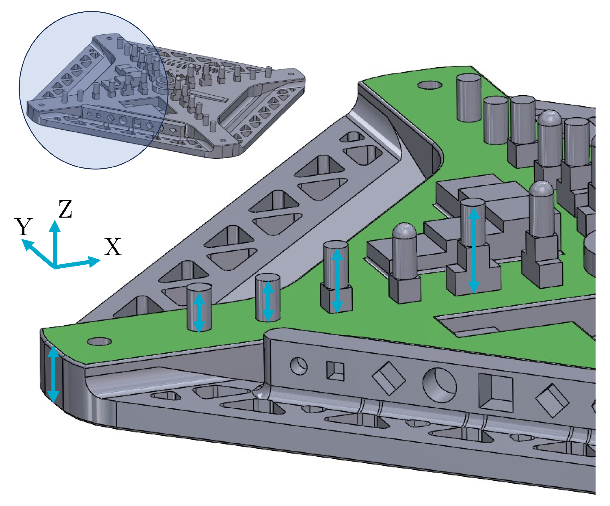
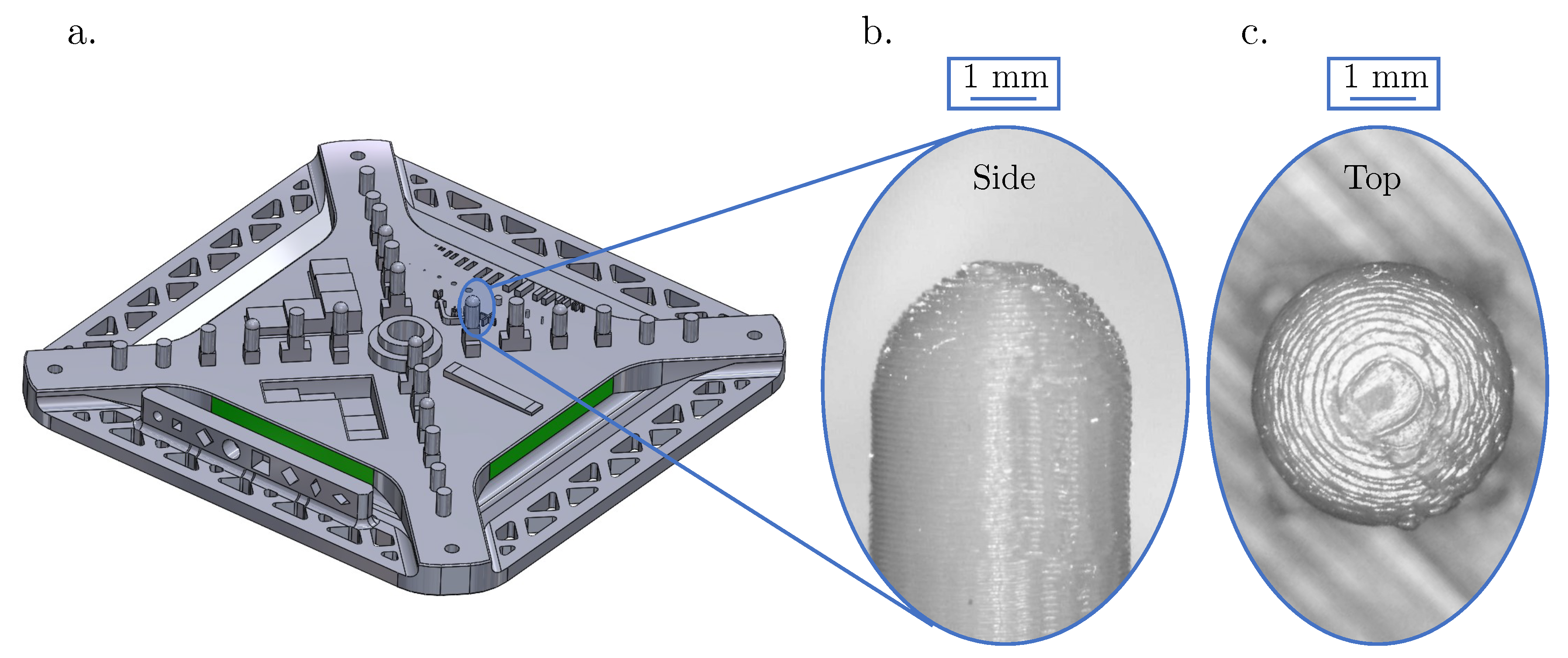
The last line in the table shows these objectives, while the last column of the table shows if each of the studies can be considered complete. As can be seen in the table, there is no existing work based on a GBTA that comprehensively assessed the machine performance of an AM printer relying on material extrusion as the FDM. Moreover, only Beltran et al. [13], Siraj et al. [47], Udroiu et al. [48], and Zongo et al. [43] made a direct link with the ISO 22514 standard in discussing and processing their results. Dolimont et al. [50], Singh et al. [46], and Yap et al. [49] relied on too low a number of measurements (<25) according to the ISO 22514 standard. Beltran et al. [13], Dolimont et al. [50], Gunay et al. [44], Preißler et al. [45], Singh et al. [46], and Siraj et al. [47] did not accurately identify the type of distribution the data belonged to but rather assumed it as normal. No study combined the dimensional and geometrical capability while ensuring a comprehensive coverage of the possible dimensions that could be obtained with the AM printer studied. Most of the existing studies focused on linear dimensions and did not encompass geometrical measurements [15]. Finally, only the Gunay et al. [44], Preißler et al. [45], Singh et al. [46], Udroiu et al. [48], and Zongo et al. [43] dealt with the standards already used in conventional processes, such as ISO 286-1 and ISO 2768, as recommended by ISO 17296-3.

4. GBTA Design

As previously mentioned, no universal GBTA exists [12]. A choice must therefore be made from among the large variety of existing GBTA designs [12,51]. The chosen design must ensure the best coverage of the ISO 286-1 dimensional size ranges achievable by the printer in its build platform while also ensuring the geometrical performance can be assessed owing to dedicated features (cylinders, hemispheres, planes, etc.). The part developed by Spitaels et al. [20] (Figure 3) can be adapted to every material extrusion printer build platform owing to an adaptive geometry. It is designed to cover, as much as possible, the available size ranges of ISO 286-1 to allow the dimensional performance to be evaluated while ensuring the geometrical performance to be assessed through cubes, cylinders, and hemispheres. Moreover, the innovative design of the part ensures a lower risk of warping, even though the part is very flat and, therefore, warping-sensitive. Finally, this part was successfully used to assess the dimensional and geometrical performance of an Ultimaker 2+ printer [20]. All of these reasons made this GBTA suitable for the planned machine performance study.

When adapted to the Ultimaker 2+ build platform, the GBTA exhibits main dimensions of 207 mm × 207 mm × 27 mm for its X, Y, and Z axes, respectively. The Z axis is along the build direction. The features included in the GBTA allow 434 dimensional and 524 geometrical measurements to be performed [20]. The dimensional measurements are distributed over the size ranges of ISO 286-1 from 1 to 3 mm and 180 to 250 mm for the X and Y axes, respectively. For the Z axis, the highest size range achieved is 18 mm–30 mm. The dimensional and geometrical measurement possibilities are further discussed in Section 6.

5. Motivation and Objective of the Study

Two recent papers demonstrate that a lot of research was previously carried out to assess the short-term performance of AM printers [12,43], while only a few works have focused on the statistic behavior of the printers for the longer term by performing a machine performance study [43]. As shown in Section 3, no study has combined a comprehensive coverage of the possible dimensions that can be obtained with the AM printer studied while using ISO 22514 to guide the treatment of the results to evaluate the dimensional and geometrical machine performance. Therefore, this study aimed to close this gap by proposing a systematic method assessing the dimensional and geometrical machine performance of material extrusion printers. The method relies on an already existing GBTA, which allows the ISO 286-1 dimensional size ranges achievable by the printer’s X and Y axes to be covered. For each feature, the best-fitting distribution (normal, log-normal, folded normal, gamma, Rayleigh, or Weibull) is identified based on a Komolgorov–Smirnov statistical test. The potential (based on $P_m$) and real (based on $P_{mk}$) tolerance intervals that the tested printer is capable of are the direct output of this study. A link was also established with the existing standards widely used for conventional processes, such as ISO 286-1 and ISO 2768, establishing which of their TI can be achieved by the printer.

6. Methods

6.1. Tested Machine and Material

The machine selected to be tested was an Ultimaker 2+. This is a material extrusion printer with a 3-axis cartesian architecture (X, Y, and Z). The build direction is given by the Z axis. It can generate parts up to 223 mm × 223 mm × 205 mm across its X, Y, and Z axes. The compatible filament feedstock is mainly polymers of polylactic acid (PLA) and acrylonitrile butadiene Sstyrene (ABS) to thermoplastic polyurethane (TPU) and polyethylene terephthalate glycol (PETG). PLA was the selected feedstock since it is easy to print and one of the most affordable. The chosen supplier for the filaments was Ultimaker. The printing parameters used to produce the GBTA are given in

Table 3. Printing parameters used to produce the parts.

Parameter	Value
Nozzle diameter [mm]	0.4
Layer thickness [mm]	0.1
Density of infill [%]	20
Type of infill	Cubic
Build platform temperature [°C]	60
Nozzle temperature [°C]	220

. These parameters were selected according to the study of Spitaels et al., presenting the selected GBTA design and also printing it on an Ultimaker 2+ with PLA filament [20]. Each part required 27 h to be printed, while their design allowed their printing without the need for a support structure [20].

6.2. Available Measurements on the GBTA

As described in the ISO 22514 standard, no less than 5 recordings should be made to assess the capability of a machine. However, in some exceptional cases, such as very slow processes or high production costs, the number of observations can be lowered to 25 [34]. With the decrease in the reliability of the observation, it is necessary to correct the $P_m$ target index to maintain a 95% confidence level [34]. Since the process characterizing (material extrusion) is very slow [3], 25 GBTAs were produced on the printer. The measurements were then grouped by the main axis and by the size ranges of ISO 286-1 and entered into a database of 10825 dimensional and 3275 geometrical measurements. The number of dimensional and geometrical measurements per axis and size range is given in

Table 4. Number of dimensional measurements among the printer axes and size ranges of ISO 286-1.

Size Range [mm]	X	Y	Z	Other
1–3	275	300	550	200
3–6	600	600	800	700
6–10	300	300	850	25
10–18	350	350	825	25
18–30	400	400	200	25
30–50	425	425	-	-
50–80	425	425	-	-
80–120	400	400	-	50
120–180	50	50	-	-
180–250	50	50	-	-

and

Table 5. Number of geometrical measurements among the printer axes and size ranges of ISO 286-1.

Type	Size Range [mm]	X	Y	Z	Other
Angularity	18–30	-	-	-	50
Coaxiality	6–10	-	-	-	50
Cylindricity	3–6	-	-	-	700
	10–18	-	-	-	50
	18–30	-	-	-	25
Flatness	6–10	-	-	300	-
	18–30	100	100	-	-
	50–80	-	-		100
	180–250	-	-	25	-
Parallelism	10–18	-	-	50	-
	18–30	75	75	50	-
	80–120	-	-	-	50
	120–180	100	100	-	-
	180–250	-	-	25	-
Perpendicularity	18–30	-	-	-	450
	50–80	-	-	-	100
	180–250	-	-	-	400
Form	3–6	-	-	-	200
Straightness	120–180	50	50	-	-

, respectively. The “Other” category refers to the measurements relying on more than one of the axes. When creating a cylinder for example in the X and Y plane, both X and Y axes awerere used to generate the geometry.

6.3. Measurement of Parts

All the parts were measured at room temperature using a Wenzel LH54 Coordinate Measuring Machine (CMM). The measurement uncertainty of the machine (in µm) for a given measurement L (in mm) for the X and Y axes was $3+L/300$, while it was $3.5+L/300$ for the Z axis. The selected spherical probe had a diameter of 1.5 mm, which allowed the staircase effect inherent to the MEX process to be filtered.

The features of the GBTA were measured, following Bourdet [52], by taking

• 8 points for each cylinder on two different circles;
• 6 points for each plane, except for the smaller ones (top of small cylinders and their parallelepiped base) which were measured by 1 point;
• 39 points for the top surface of the parts;
• 9 points on 3 circles for the hemispheres.

The CMM was piloted using Metrosoft QUARTIS Measurement Software (version 2021). This software allowed the measurements to be performed automatically. Each part required about 1 h to be measured and was evaluated once. Measuring the parts was performed at least 24 h after their fabrication and removal from the build platform. No postprocessing operation was applied.

6.4. Data Postprocessing

Several steps were followed to postprocess the data according to the ISO 22514 standard:

• Grouping data: First, the dimensional data were grouped according to their size range and their main reference axis (the dimensions between 3 mm and 6 mm for the X axis, for example). Each of the different geometrical data types were also grouped in the same way (the flatness of planes with a normal according to the X axis and exhibiting a main dimension between 18 mm and 30 mm, for example).
• Retrieving the deviation: The deviation from the nominal value was computed ($Dat{a}_{deviation}$) by retrieving the nominal size ($Dat{a}_{nominalsize}$) from the measured data ($Dat{a}_{measured}$) as shown in Equation (7). For example, a diameter with a 4 mm nominal value measured at 4.174 mm gave a 0.174 mm deviation.

  $$Dat{a}_{deviation}=Dat{a}_{measured}-Dat{a}_{nominalsize}$$

  (7)
• Histogram shape check: The shape of the data distribution was then checked by plotting a histogram. This plot allowed the outliers to be detected and manually discarded. The general shape of the histogram also revealed the possible multimodal distribution of the data in some cases. When this happened, a manual separation of the data was performed to identify the different contributions. These datasets were then separately processed for the next operations.
• Distribution fitting: The histogram allowed the general shape of the distribution to be identified. In some cases, the data could not be estimated by a normal distribution. According to the ISO 22514 standard, the data can fit to a normal, log-normal, folded normal, gamma, Rayleigh, or Weibull distribution depending on their nature. Therefore, a fitting of the dataset with these six different statistical distributions was performed. The best fitting distribution was identified using the p-value of a Komolgorov–Smirnov test for each dataset. The distributions were chosen following the highest achieved p-value.
• Indices computation: The $X_{0.135\%}$, $X_{50\%}$ and $X_{99.865\%}$ percentiles were then computed to allow the machine performance indices to be obtained. Finally, the $P_m$ and $P_{mk}$ estimates were computed according to ISO 22514 with a confidence level of 95%. This value was chosen according to Bissel [35] and Chou et al. [36].

7. Results and Discussion

7.1. Application of the Method to a Dataset

Figure 4 gives the results of the fitting applied to the dimensional data belonging to the Y axis of the printer from 3 mm to 6 mm.

• Grouping data: A total of 600 measurements were available in this group (in blue in the figure), and these encompassed the distances between the planes.
• Retrieving the deviation: The deviations with respect to the nominal value were computed according to Equation (7).
• Histogram shape check: As shown in blue in Figure 4, the histogram does not show outliers and is not multimodal. The measurements, therefore, did not need to be separated.
• Distribution fitting: The six different distributions were tested for the fitting, and the best selected was the Weibull distribution, with a computed p-value from the Komolgorov–Smirnov test reaching 0.998. The resulting distribution is given in orange on the graph and fits the data histogram very well.
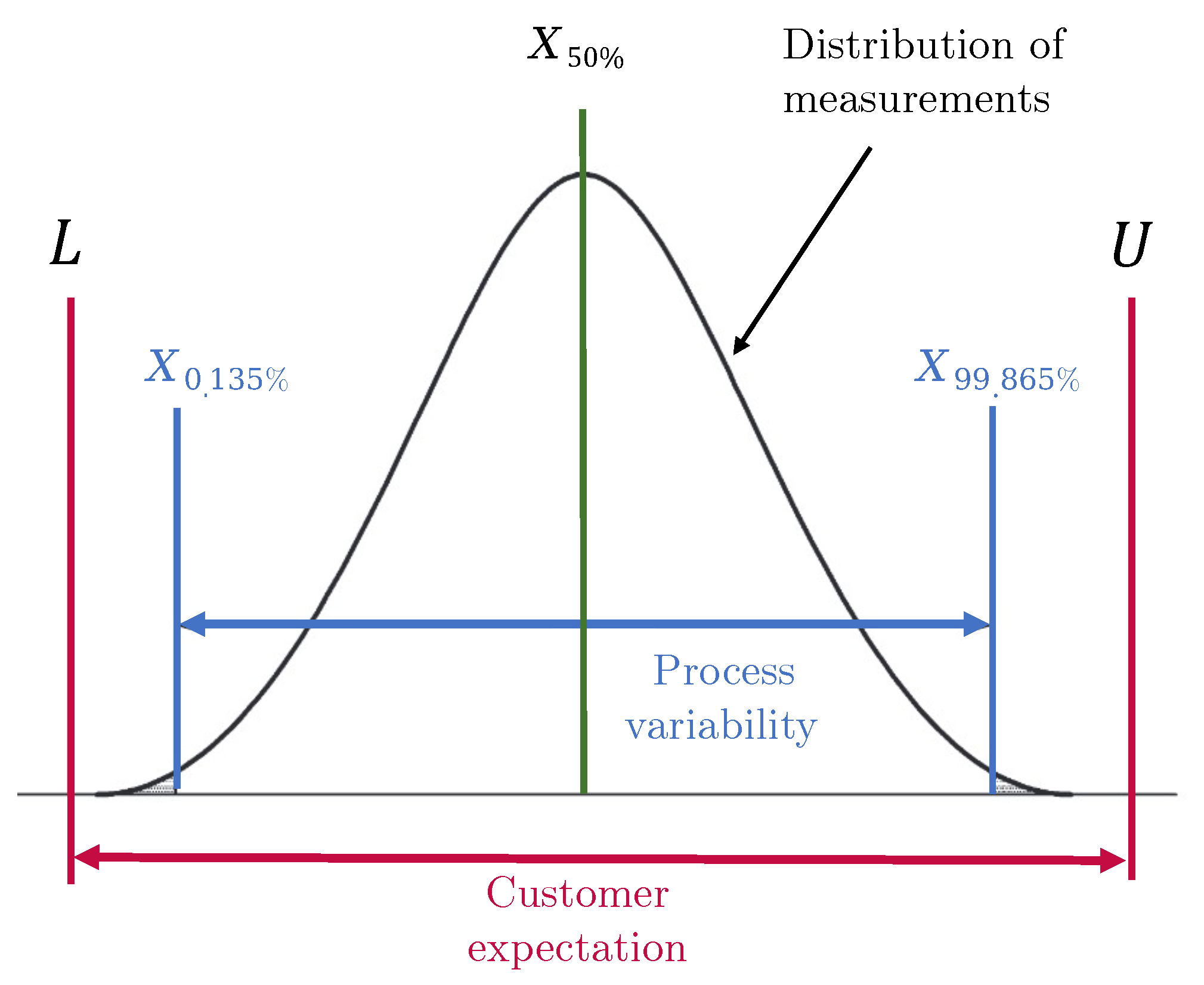
• Index computation: The obtained $X_{0.135\%}$, $X_{50\%}$ and $X_{99.865\%}$ percentiles were, respectively, −0.027 mm, 0.058 mm and 0.123 mm. Finally, the tolerance interval achieved by the machine could be computed. No correction was needed for $P_m$ since the number of measurements was above 50. Consequently, a potential tolerance interval of 0.251 mm was obtained for a $P_m$ of 1.67. Using the same target for $P_{mk}$, the lower (L) and upper (U) bounds of the real tolerance interval could be determined: −0.082 mm and 0.163 mm, respectively. The asymmetry of the real tolerance interval was confirmed with the median value, which was 0.058 mm instead of 0 mm. As depicted in Figure 4, the data slightly shifted to the right on the graph.

7.2. Distribution Identification

As explained in the ISO 22514 standard, the distribution that best fits the data is not only normal. Depending on the type of measurement (dimensional and geometrical), different distributions can be suitable for fitting the datasets. Figure 5 and Figure 6 give the repartition of the chosen distribution for the dimensional and geometrical measurements, respectively. As can be seen in Figure 5, the majority of the dimensional data (57.9%) could be described using a normal distribution. However, almost one-quarter of the data (24.6%) needed to be fitted with a nonsymmetrical distribution, such as a gamma distribution. The second most used nonsymmetrical distribution was the log-normal, with 7% of measurements.

In terms of geometrical measurements, the normal distribution fitting was only suitable for 24.3% of the data, while the log-normal and gamma allowed 33.3% and 21.2% of the data to be represented, respectively. This is in accordance with ISO 22514. One-sided specifications, like geometrical measurements (e.g., flatness), mostly require a nonsymmetrical distribution. Moreover, it is not possible to have negative values for geometrical measurements, meaning that using more log-normal distributions is to be expected.

The distribution fitting the data was chosen taking the highest computed Komolgorov–Smirnov p-value between the different possible distributions. However, for some measurements, the difference in terms of p-value was very low, meaning that different distributions could fit the data. For example, the measurements along the Z axis from 10 mm to 18 mm exhibited a p-value for the normal, Weibull, and log-normal distributions of 0.931, 0.949, and 0.952, respectively. As a result, the log-normal distribution was chosen to fit the data and compute the $X_{0.135\%}$, $X_{50\%}$, and $X_{99.865\%}$ percentiles. Nevertheless, the Weibull distribution, or even the normal distribution, could have been suitable for computing them since the p-value was higher than the 0.05 level. This was expected since a log-normal or a Weibull distribution with tuned parameters can approximate a normal distribution. However, only a few papers provide detail about the distribution identification and normal suitability verification [42,43,48,49]; most of the other studies assumed a Normal distribution without verifying it. The presented results demonstrate the necessity of conducting a more in-depth analysis of the distribution identification prior to choosing one and computing the required percentiles.

7.3. Dimensional Machine Performances Assessment

7.3.1. Potential Dimensional Tolerance Intervals

The previously presented method was applied to all the measured dimensional data, which allowed the potential tolerance intervals to be determined. The results are depicted in Figure 7. The horizontal axis gives the dimensional size ranges of ISO 286-1 (in mm), while the plotted data show, for each machine axis, the potential TI (in mm) ensuring $P_m=1.67$. As the printer had a three-axis Cartesian architecture, three axis categories were considered: X, Y, and Z (the real machine axes). A supplementary category named Other was added to take into account the combinations of axes. Dimensions referring to this category are, for example, the cylinder diameters. Indeed, to be generated, a cylinder needs two axes to be used instead of one (in the case of a plane, for example). The error bars limit the interval for which $P_m$ is estimated to ensure 95% confidence.

As depicted in Figure 7, except for features with dimensions between 6 mm and 10 mm, the X and Y axes exhibited a better performance than the Z axis. However, the computed TI did not strictly increase with the dimensional size ranges of ISO 286-1. For example, the computed X and Y axes’ TI for the size ranges of 10 mm to 30 mm w4ere lower than the TI for the size range between 6 mm and 10 mm. This was from the type of measurements in these size ranges. The nature of the measurements used in the dimensional study is shown in

Table 6. Type of measurements used in the dimensional study for the different axes and size ranges: cylinder-to-cylinder (Cyl.), plane-to-plane (Planes), and plane-to-cylinder (Combi.) distances.

	X			Y			Z	Other
Sizes [mm]	Cyl.	Planes	Combi.	Cyl.	Planes	Combi.	Planes	Cyl.	Planes
1–3	0%	100%	0%	0%	100%	0%	100%	0%	0%
3–6	0%	100%	0%	0%	100%	0%	100%	100%	0%
6–10	0%	83%	17%	0%	83%	17%	100%	100%	0%
10–18	100%	0%	0%	100%	0%	0%	100%	100%	0%
18–30	75%	13%	13%	75%	13%	13%	100%	100%	0%
30–50	53%	24%	24%	53%	24%	24%	-	-	-
50–80	76%	0%	24%	76%	0%	24%	-	-	-
80–120	25%	50%	25%	25%	50%	25%	-	0%	100%
120–180	100%	0%	0%	100%	0%	0%	-	-	-
180–250	50%	50%	0%	50%	50%	0%	-	-	-

. It shows, for the different dimensional size ranges and axes, the relative proportion of plane-to-plane (Planes), cylinder-to-cylinder (Cyl.), and plane-to-cylinder (Combi.) distances.

Considering the X and Y axes, from 6 mm to 10 mm, the majority of the measurements were plane-to-plane distances (about 83%), while from 10 mm to 18 mm, the measurements were composed exclusively of cylinder-to-cylinder distances. From 18 mm to 30 mm, the measurements were composed of a mix of plane-to-plane distances (about 13%) and cylinder-to-cylinder distances (about 75%); the rest of the measurements (about 13%) relied on plane-to-cylinder distances. This example shows the sensitivity of the method to the design of the features that are printed. Therefore, in the design phase of a part, this should be considered to obtain a reliable TI depending on the geometry to be produced.

The computed tolerances can be used by designers to foresee the fitting between parts shaped using the tested machine. Another application could be the determination of machining stock allowance, if the parts are milled after printing, for example. However, since the results are sensitive to the type of features measured, it means that the GBTA part should be modified in accordance with the type of part being produced. Indeed, if the majority of the part that is being produced exhibits planar surfaces, the selected GBTA could then be modified by replacing the small cylinders on its top surface with a parallelepiped with dimensions equivalent to their diameter. This is a drawback of the selected GBTA design. Nevertheless, as explained by de Pastre et al. [12], it is not possible to have a universal GBTA design.

As displayed in Figure 7, the tolerance intervals are very large, with values up to 0.753 mm for a dimensional measurement along the X axis with dimensions between 30 mm and 50 mm. Since $P_m=1.67$ is the capability index target, it ensures a confidence level of 95% with less than 0.6 nonconforming parts per million. Therefore, depending on the application foreseen for the part, the target for $P_m$ can be adjusted and lowered if a larger number of nonconforming parts is allowed. In addition, care should be taken when using these TIs: they are the potential TI the machine can achieve and not the real ones, since $P_m$ allows the potential machine capability to be determined and does not take into account the position of the results between the lower and upper bounds of the TI.

The method was also applied to the same dataset but considering a $P_m$ target of one. The results are depicted in Figure 8, and the resulting potential TIs are about half of the TI computed with the $P_m$ target at $1.67$. As presented in Table 1, the potential number of out-of-specification parts for this target, if the measurements can be expressed using a normal distribution, stands at 2600 per million produced. Therefore, this cannot be used in the case of critical applications (biomedical implants or components for the nuclear industry, for example), where the cost of such a potential quantity of out-of-specification parts is too high. Nevertheless, these tolerance intervals can be suited to prototyping purposes or other applications that do not require much precision or for which the cost for the management of out-of-specification parts is low.

7.3.2. Real Dimensional Tolerance Intervals

By isolating the L and U values in Equation (2), it is possible to compute the lower (L) and upper (U) tolerance interval bounds. The resulting intervals are given in

Table 7. Tolerance intervals: lower (L) and upper (U) bounds for $P_{mk}$ = $1.67$ at a confidence level of 95%.

	X		Y		Z		Other
Size [mm]	L [mm]	U [mm]	L [mm]	U [mm]	L [mm]	U [mm]	L [mm]	U [mm]
1–3	−0.112	0.100	−0.142	0.148	−0.233	0.233	−0.055	0.082
3–6	−0.111	0.179	−0.082	0.163	−0.191	0.299	−0.147	0.083
6–10	−0.228	0.197	−0.317	0.352	−0.211	0.241	−0.177	−0.098
10–18	−0.096	0.050	−0.138	0.080	−0.095	0.577	−0.039	0.138
18–30	−0.085	0.045	−0.194	0.135	0.042	0.792	−0.052	0.110
30–50	−0.355	0.398	−0.159	0.328	-	-	-	-
50–80	−0.341	0.638	−0.041	0.248	-	-	-	-
80–120	−0.734	0.270	−0.357	0.332	-	-	−0.589	−0.180
120–180	−0.048	0.130	−0.120	0.310	-	-	-	-
180–250	−1.021	−0.112	−0.979	0.455	-	-	-	-

for a targeted $P_{mk}$ value of $1.67$ and a confidence level of 95%. In this table, it is possible to identify if the tolerance intervals are shifted or not.

In the case of dimensions between 6 mm and 10 mm belonging to the Y axis, the lower bound is located at -0.317 mm while the upper bound is located at 0.352 mm. Consequently, the center of the TI is located at 0.035 mm, which is very close to 0 mm, which is the initial targeted value. Conversely, some other intervals are shifted, as in the case of dimensions between 10 mm and 18 mm belonging to the Z axis. The lower bound is at −0.095 mm, while the upper bound is at 0.577 mm. The middle of the TI is then located at 0.482 mm, meaning that these features exhibit a dimension on average 0.482 mm longer than the nominal size. The measured shift can be seen as a systematic error and could be compensated for using software when designing the part to be printed.

These are the real tolerance intervals used for foreseeing the fittings between the parts printed on the tested printer with the same parameters. Again, the design of the desired parts should be taken into account since it has an influence, as previously demonstrated.

7.3.3. Potential Achievable STG of ISO 286-1

As explained in the Introduction, ISO 286-1 is recommended for usedwhen characterizing AM parts. Consequently, its standard tolerance grades (STG) were considered, and the developed method was used to determine which STG can be reached using the selected printer.

Table 8. Potential ISO 286-1 STG with $P_m=1.67$ and a 95% level of confidence.

Size [mm]	X	Y	Z	Other
1–3	IT 14	IT 15	IT 16	IT 14
3–6	IT 14	IT 14	IT 16	IT 14
6–10	IT 15	IT 16	IT 15	IT 12
10–18	IT 11	IT 13	IT 15	IT 13
18–30	IT 12	IT 13	IT 15	IT 13
30–50	IT 15	IT 14	-	-
50–80	IT 15	IT 13	-	-
80–120	IT 14	IT 14	-	IT 13
120–180	IT 11	IT 13	-	-
180–250	IT 14	IT 15	-	-

shows the results of this analysis by giving, for the different dimensional size ranges of ISO 286-1 and the features orientations with respect to the printer axes (X, Y, Z, and their combination called Other), the potential STG that guarantees a $P_m$ of $1.67$. The same 95% level of confidence was considered for the computations.

The same conclusions were drawn regarding the relative performance of the different axes: the X and Y axers perform better than the Z axis. Indeed, the lower the STG, the narrower the tolerance interval. Again, the feature design sensitivity can be observed for the size ranges. Between 6 mm and 10 mm and between 10 mm and 18 mm for the X axis, the achieved STGs are IT 11 and IT 15, respectively. Again, the type of measured features influences the evaluated performance of the printer. As before, the $P_m$ target of $1.67$ can be challenged depending on the final application of the produced parts.

7.3.4. Real Achievable STG of ISO 286-1

With the already existing tolerance intervals, it is possible to compute the $P_{mk}$ index and, consequently, the real achievable tolerance intervals. The results of this analysis for a $P_{mk}$ target of 1.67 at a confidence level of 95% are given in

Table 9. Potential (Pot.) and real (Real) STGs and their difference (Diff.) for $P_{mk}=1.67$ at a confidence level of 95%. Color code for the Diff. column: no difference in STG in green, difference of one STG in yellow, difference of two STGs in orange, and difference of three STGs in red.

	X			Y			Z			Other
Size [mm]	Pot.	Real	Diff.	Pot.	Real	Diff.	Pot.	Real	Diff.	Pot.	Real	Diff.
1–3	IT 14	IT 14	0	IT 15	IT 15	0	IT 16	IT 16	0	IT 14	IT 14	0
3–6	IT 14	IT 15	1	IT 14	IT 15	1	IT 16	IT 16	0	IT 14	IT 14	0
6–10	IT 15	IT 15	0	IT 16	IT 16	0	IT 15	IT 16	1	IT 12	IT 15	3
10–18	IT 11	IT 12	1	IT 13	IT 14	1	IT 15	IT 17	2	IT 13	IT 14	1
18–30	IT 12	IT 13	1	IT 13	IT 14	1	IT 15	IT 17	2	IT 13	IT 13	0
30–50	IT 15	IT 15	0	IT 14	IT 15	1	-	-	-	-	-	-
50–80	IT 15	IT 16	1	IT 13	IT 14	1	-	-	-	-	-	-
80–120	IT 14	IT 15	1	IT 14	IT 15	1	-	-	-	IT 13	IT 15	2
120–180	IT 11	IT 12	1	IT 13	IT 14	1	-	-	-	-	-	-
180–250	IT 14	IT 16	2	IT 15	IT 16	1	-	-	-	-	-	-

. It gives the potential (Pot.) and real (Real) STG achieved as well as an index (Diff.) showing if there is a one, two, or three STG difference between the potential and real STG. As can be seen, most of the real STGs are higher than the potential ones, meaning that the real tolerance intervals are higher than the potential. This shows the necessity of taking into account the potential shift in the measurement distribution from the TI center to guarantee the $1.67$ machine performance target. Nevertheless, the observed STG difference should not be considered alone since the shift can occur in two different directions (real STG begins higher or lower than the potential).

Some results exhibited a two STG IT difference for the Z axis. This again originates from the design of the part. Indeed, these measurements are composed mainly of the distance between the GBTA base surface (the one in contact with the build platform during printing) and the planes on top of the small cylinders. Since the part is wide in the X and Y directions and relatively flat, it is subjected to slight warping deformations. Even with the innovative design introduced by Spitaels et al. [20], the part deforms slightly after cooling and exhibits small permanent deformations, which can induce a systematic shift between the height target and the real one. Indeed, the average flatness measured with 40 points on the GBTA top surface of the part (in green in Figure 9) over the 25 produced GBTA was 0.137 mm with a standard deviation of 0.049 mm. This could have influenced the results and led to a shift between the desired dimensions and the real ones.

Only one measurement type exhibited a very high difference between the potential STG and the real one (three STGs IT of difference in red in Table 9). The features of these measurements belong to the 6 mm to 10 mm dimensional size range and depend on a combination of the machine axes (“Other” category in the table). These measurements are the measured diameter of the central cylinder (nominal diameter of 10 mm), as circled in Figure 10 in green. The central bore was on average 0.149 mm too small, as shown in Figure 11 (central category in green). This figure shows the relative deviation from the nominal value of the diameter of the GBTA cylinders (negative value represents a lower diameter).

This tendency could be compared to the other available bores of 4 mm (in orange, grey, blue, and yellow in Figure 10) at the end of the adaptive arms forming the GBTA (3 mm to 6 mm, Other, in Table 9). These were on average 0.181 mm too small, as shown in Figure 11 for the X−, X+, Y−, and Y+ categories. These categories are related to the positions of the bore with respect to the GBTA axes. Therefore, X− refers to the bore at the end of the arm parallel to the X axis of the printer with a negative orientation.

However, the effect of this shift is not seen in Table 9 due to several effect.s First, these measurements are not the only ones belonging to the 3 mm to 6 mm range and Other class. Indeed, they represent only 100 measurements over the 700 available. As a result, their effect is hidden by the better performance of the other 600 measurements. Moreover, the 6 mm to 10 mm range and Other class only contain 25 measurements since there was only one central bore for each GBTA. Therefore, the $P_{mk}$ target was raised to $1.86$ instead of $1.67$ to ensure the 95% confidence level was met. This worsened the effect of the measured deviation.

In general, the bores measured on the GBTA had a smaller diameter than desired. Indeed, as it can be seen in Figure 11, all the deviations in the results were lower than the target. Some slight differences can be seen in the graph, with higher deviations in the case of the Y− category, slightly better results for the X− and X+ categories, and the best results among the displayed data for the Y+ category. The depicted measurement dispersion was from the measurement uncertainty of the CMM. Even if the results were in the same range, it should be noted that the X-axis cylinders (categories X− and X+) exhibited more homogeneous results, while those ones belonging to the Y axis (categories Y− and Y+) were less homogeneous. Finally, taking into account the size of the measured features, the 4 mm diameter bores exhibited higher deviations than the 10 mm bore. This was a consequence of the design and the printing parameters. Indeed, the effect of the selected layer thickness (0.1 mm) should have been stronger for the 4 mm bores (depth of 10 mm) compared to the 10 mm bores (depth of 17 mm). This could also explain the better homogeneity of results for the 10 mm bore compared to each of the X−, X+, Y−, and Y+ categories.

From a conception point of view and depending on the foreseen application, this shift in diameter for the bores can be a real problem if it is not anticipated. If a fit between a shaft and a bore is foreseen, the best solution should be to compensate for the systematic error of the printer by applying a correction to the diameter of the bores in the CAD file. In the case of GBTA bores, it should be a slight increase in the bore nominal diameter since all the bore diameters were lower than the nominal size.

7.4. Geometrical Machine Performance Assessment

7.4.1. Real Geometrical Tolerance Intervals

The described method was also applied for the geometrical measurement of the GBTA. In this case, the tolerance intervals were unilateral. Therefore, only the $P_{mk}$ index was computed, leading to the upper bound (U) of the real geometrical tolerance interval. Indeed, in the case of geometrical measurements, there is no lower bound since the targeted value is 0, while a negative value for a geometrical deviation type (e.g., flatness) does not have any physical meaning. Two targets of $P_{mk}$ were used as before: $1.67$ and 1. The resulting TIs are given in

Table 10. Real geometrical tolerance intervals (TIs) in mm for $P_{mk}=1.67$ and $P_{mk}=1$ with their lower (LL) and upper (UL) limits in mm ensuring a 95% confidence level.

			${\mathit{P}}_{\mathit{m}\mathit{k}}$ = 1.67			${\mathit{P}}_{\mathit{m}\mathit{k}}$ = 1
Type Geo.	Axis	Size [mm]	TI [mm]	LL [mm]	UL [mm]	TI [mm]	LL [mm]	UL [mm]
Angularity	Other	18–30	0.137	0.110	0.164	0.086	0.066	0.098
Coaxiality	Other	6–10	1.833	1.471	2.194	1.143	0.881	1.314
Cylindricity	Other	3–6	0.144	0.136	0.152	0.088	0.082	0.091
	Other	10–18	0.063	0.051	0.076	0.082	0.030	0.045
	Other	18–30	0.043	0.031	0.055	0.028	0.019	0.033
Flatness	Other	50–80	0.360	0.310	0.410	0.220	0.186	0.246
	X	18–30	0.023	0.020	0.026	0.014	0.012	0.016
	Y	18–30	0.046	0.039	0.052	0.028	0.024	0.031
	Z	6–10	0.040	0.037	0.043	0.045	0.022	0.026
	Z	180–250	0.412	0.296	0.528	0.268	0.178	0.316
Parallelism	Other	80–120	0.110	0.088	0.132	0.143	0.053	0.079
	X	18–30	0.115	0.096	0.133	0.153	0.058	0.080
	X	120–180	0.088	0.076	0.100	0.109	0.045	0.060
	Y	18–30	0.114	0.095	0.132	0.070	0.057	0.079
	Y	120–180	0.104	0.090	0.119	0.130	0.054	0.071
	Z	10–18	0.034	0.027	0.041	0.021	0.016	0.024
	Z	18–30	0.034	0.027	0.041	0.021	0.016	0.024
	Z	180–250	0.606	0.436	0.777	0.395	0.261	0.465
Perpendicularity	Other	18–30	0.084	0.079	0.090	0.120	0.047	0.054
	Other	50–80	0.069	0.059	0.079	0.091	0.036	0.047
	Other	180–250	0.122	0.113	0.130	0.154	0.068	0.078
Form	Other	3–6	0.288	0.260	0.316	0.176	0.156	0.189
Straightness	X	120–180	0.065	0.052	0.078	0.042	0.031	0.047
	Y	120–180	0.068	0.054	0.081	0.045	0.032	0.048

as well as the lower (LL) and upper (UL) limits of the confidence level guaranteeing the $P_{mk}$ is estimated with 95% reliability. The left part of the table shows the results for $P_{mk}=1.67$, while the right part gives the same information but for $P_{mk}=1$. The same size ranges as ISO 286-1 were considered.

The coaxiality was the highest deviation produced by the printer, with a 1.833 mm deviation, ensuring the machine is capable at a $P_{mk}=1.67$. Again, this was from the GBTA design, which exhibits cylinders (at its center) with a large diameter (10 mm, 15 mm, and 20 mm) compared to their height (17 mm, 3 mm, and 4 mm, respectively). Consequently, this makes the measurement of coaxility very sensitive and leads to a very large TI to ensure the printer is capable.

The next highest TIs were for the parallelism of planes with dimensions between 180 mm and 250 mm according to the Z axis (0.606 mm, while ensuring $P_{mk}=1.67$), followed by the flatness of planes of the same axis and dimensions (0.412 mm). Parallelism was evaluated for the bottom surface of the part and its top surface (presented in green in Figure 9), while the flatness was evaluated for the GBTA’s top surface. In both cases, only one measurement was available for each GBTA, leading to 25 measurements of the printed parts. Consequently, the $P_{mk}$ target had to be raised from $1.67$ to $1.87$ for both. This led to an overestimation of the tolerance interval since a confidence level of 95% was chosen. Moreover, the spread of the measurements was broad, with an $X_{99.865\%}$ percentile at 0.545 mm, while the median was 0.223 mm. This showed less repeatability for the measurement and a weaker ability of the printer to generate the desired geometry.

Finally, the two other highest tolerance intervals were for the flatness of planes with dimensions between 50 mm and 80 mm combining several axes (Other category with 0.360 mm) and the form error of the 2 mm radius hemispheres on top of the small 4 mm positive cylinders. The flatness measurements were conducted with the vertical planes shown in Figure 12a (in green). Despite the high number of available measurements (100, as depicted in Table 5), the poor resulting flatness originated again from the spread of the measurements. As before, it was broad, with the $X_{99.865\%}$ percentile at 0.312 mm and a median at 0.092 mm. Finally, the large form error associated with the hemispheres was from the printing parameters. Indeed, they exhibited a nominal radius of 2 mm, while the chosen layer thickness was 0.1 mm. This means that only 20 layers were created by the printer to produce the hemispheres. A low number of layers with a curved surface results in a relatively pronounced staircase effect. This effect can be seen in Figure 12b,c.

Again, the method is sensitive to the design of the features as well as the printing parameters and the process limitations. As before, the $P_{mk}=1.67$ target can be challenged depending on the final application of the parts. The right part of Table 10 gives the resulting TI for a $P_{mk}$ target of one. As before, the TIs are lower but at a higher risk of generating out-of-specification parts (2600 potential defective parts per million produced). Since only the $P_{mk}$ target was modified, the previous conclusion and ranking of higher deviations were still valid; only the values of the tolerance intervals changed.

7.4.2. Real Achievable Geometrical Tolerances of ISO 2768-2

As before, the performance of the printer was compared to the already existing standards whose tolerance intervals are already known. For geometrical measurements, ISO 17296-3 recommends using the ISO 2768-2 standard, which is dedicated to subtractive processes, such as machining. This standard gives three levels of tolerance: fine (H), medium (K), and large (L). However, the standard only addresses these tolerance intervals to the flatness, parallelism, perpendicularity, and straightness measured on the parts. Therefore, only these geometrical measurements were evaluated using this standard.

Again, a $P_{mk}$ target value of 1.67 was considered as well as a 95% confidence level. The results of the analysis are given in

Table 11. Real levels of geometrical tolerance according to ISO 2768-2: fine (H), medium (K), large (L). Other symbols: not capable (NC) and absence of available measurement (dash).

Type	Size [mm]	X	Y	Z	Other
Flatness	1–10	-	-	L	-
	10–30	H	H	-	-
	30–100	-	-	-	NC
	100–300	-	-	L
Parallelism	1–10	-	-	-	-
	10–30	NC	NC	K	-
	30–100	-	-	-	L
	100–300	H	K	NC	-
Perpendicularity	1–100	-	-	-	H
	100–300	-	-	-	H
Straightness	100–300	H	H	-	-

, a dash represents the absence of an available measurement, while NC stands for not capable. The size ranges of ISO 2768-2 are larger than those of ISO 286-1. This is a limitation of the standard. Indeed, its size ranges aggregate more results, decreasing the ease of identifying which features cause the computed larger deviations. However, as before, the larger deviations originated from the parallelism of planes with dimensions between 30 mm and 100 mm using several axes to be generated (Other category) and from the flatness of planes with a normal oriented following the Z axis of the printer and dimensions between 100 mm and 300 mm. The last one was the flatness of planes according to the Z axis and with dimensions between 1 mm and 10 mm. Since classes were considered, there was a risk of obtaining a result very near the lower bound of one level of tolerance without noticing it. This was the case for these planes. They were just higher than the medium level of tolerance K and, consequently, belonged to the large level of tolerance L.

Some features lead to the inability of the printer to fullfil the tolerances of ISO 2768-2. The parallelism of planes between 10 mm and 30 mm for the X and Y axes cannot reach the $P_{mk}$ = 1.67 target even for the large level of tolerance (L). The same conclusion could be drawn for the parallelism of planes with dimensions between 100 mm and 300 mm belonging to the Z axis. Finally, for the flatness of planes with dimensions between 30 mm and 100 mm depending on several axes, the printer was also considered not capable.

This analysis is useful for comparing the performance of the printer with already existing standards. However, as explained, this analysis cannot estimate the machine’s performance for all possible geometrical deviations since the standard is limited to flatness, parallelism, perpendicularity, and straightness. Moreover, the analysis may be less precise than the determination of the real geometrical tolerance intervals, as, additionally, the use of a level of tolerance once again decreases the precision of the analysis. Nevertheless, this is a relevant complementary analysis that enables the performance of the printer to be compared with other existing processes. Finally, the design of the GBTA is not able to cover all the existing size ranges of the possible geometrical deviations. Again, as presented by de Pastre et al. [12], this is a consequence of the impossibility of having a universal GBTA.

7.5. Future Challenges and Potential Prospects

The proposed method is able to capture the machine performance of the tested AM printer. However, it focuses on the consequences of the machine’s inaccuracies and does not correct the process or part design. The future challenges and potential prospects in that field are addressed in the following paragraphs.

Metrology for AM parts, especially for complex designs (such as lattice), is still a challenge since conventional measuring means are limited to simple designs, while new techniques still require standardization [11]. Therefore, the choice of a CMM for measuring the GBTA parts could be challenging for future developments. Indeed, the metrology for AM parts is relying more and more on noncontact techniques such as triangulation, photogrammetry, and X-ray computed tomography (XCT) [11,53]. These techniques allow the evaluation of complex shapes. However, the traceability and comparability of the measurements is still a challenge and the subject of extensive research [11]. The number of points probed by the CMM was chosen to keep the measurement time relatively low. A future perspective on the current work would then be to use optical measurement means to provide a larger set of points and better model the part’s deviations, while keeping the measuring time short. Combining this set of data with a modal representation method of geometrical deviation decomposition, such as the one described by Dantan et al. [15], could provide an interesting evaluation of the observed deviations. Indeed, this research team proposed decomposeing the final printed geometry into several modes of deformation of the desired nominal surface. In their sudy, they concluded that the three main modes causing the observed deformations were due to

• The shrinkage of the part after its cool-down (radius mode);
• The control of the machine movements (ellipse mode);
• The geometrical defects of the machine itself (gap mode).

Their approach also relied on a material extrusion printer but one that only had cylinders ranging from 10 mm to 30 mm. Measuring the GBTA with a larger number of points could be an interesting solution to decompose its deformations modes and provide a model predicting its deformations. A compensation at the design stage to reduce the process variability could then be applied that would allow more repeatable and predictable shapes to be produced. This has the potential to enhance the performance indices that can be achieved by the printer. For this purpose, Huang et al. [54] proposed a solution based on the modification of the CAD file prior to its manufacturing to compensate for its geometrical deviations. Extending this method to more complex part geometries, such as the proposed GBTA encompassing a systematic coverage of ISO 286-1 dimensional size ranges, could entail more complete approach. Moreover, the influence of the STL mesh parameters (number of triangles, surface, and volume of thee CAD model) on the final part geometry cannot be neglected in some cases [55]. Even when a strong correlation was established between these parameters and the final dimensional characteristics of the part, only a simple design was analyzed (dog bone tensile samples from ISO 527-2) [55]. Extending this analysis to more complex parts such as the GBTA could also be of interest.

Instead of using a model to predict and compensate for the part deviations at the design stage (offline approach), monitoring the process and the part construction during the process (online approach) can be another alternative. Some attempts, such as by Cohen et al. [56], were made to monitor the whole construction of the part instead of lower-level process variables (e.g., print head temperature, material flow rate). The main advantage of this method is its lower cost since it needs only height measurements performed using a laser triangulation sensor, while other methods require many more sensors [56]. However, even if vision tools for AM are advancing, many approaches still rely on lower-level process parameters [57]. They monitor the process variables, detect their anomalies, and compensate for their deviations during the part’s construction using a closed-loop controller, such as the common proportional-integral derivative (PID) [57,58]. However, especially in polymer AM, the defects’ root causes may be very complex to establish since many factors influence them [57]. New and emerging decision-making tools such as artificial intelligence (AI) may be promising solutions to better dimension and tune the controllers and adequately compensate for the process deviations [57]. This is still a hot topic that will require extended research in the coming years.

The capability of only one machine was evaluated with the developed method. Extending this analysis to several machines of the same type would be of great interest. Indeed, part inaccuracy and AM variability across multiple machines remains poorly covered in the literature, as stated by McGregor et al. in a recent paper [53]. This research team studied the variabilities that can be observed on polymer parts produced using three identical vat polymerization printers. Again, the dimensions covered by the parts printed were reduced (from 0.5 mm to 12.5 mm). Reproducing and measuring the proposed GBTA on several printers of the same type may then be of interest. However, the current literature does not exhibit a method of easily displaying and ranking the performance of several printers. Creating a global indicator for the dimensional and geometrical performance could solve this issue and ease the use of performance information from the R&D office to workshops.

The printing parameters considered in this study were chosen according to the study of Spitaels et al., which presented the selected GBTA design. However, the accuracy of 3D-printed features depends on their geometry as well as on their printing conditions [59]. The GBTA used in this study as well as the developed method relying on machine performance indices allowed us to more deeply investigate this conclusion. Therefore, a direct application of this study could be performing a machine performance assessment while integrating variations in the printing parameters. Different performance results may be obtained depending on the selected printing parameters. Finally, optimizing the parameters with the method described by Papazetis and Vosniakos [60] could reduce the production time of the GBTA, while producing more uniform deposited strands and enhanced printer performance.

8. Conclusions

This paper presented a systematic method based on a GBTA and the prescriptions in ISO 22514 to assess the machine performance of material extrusion printers. This method was applied to an Ultimaker 2+ printer using 25 GBTA parts, creating a large dataset of 10,825 dimensional and 3275 geometrical measurements.

The main conclusions of the study are as follows:

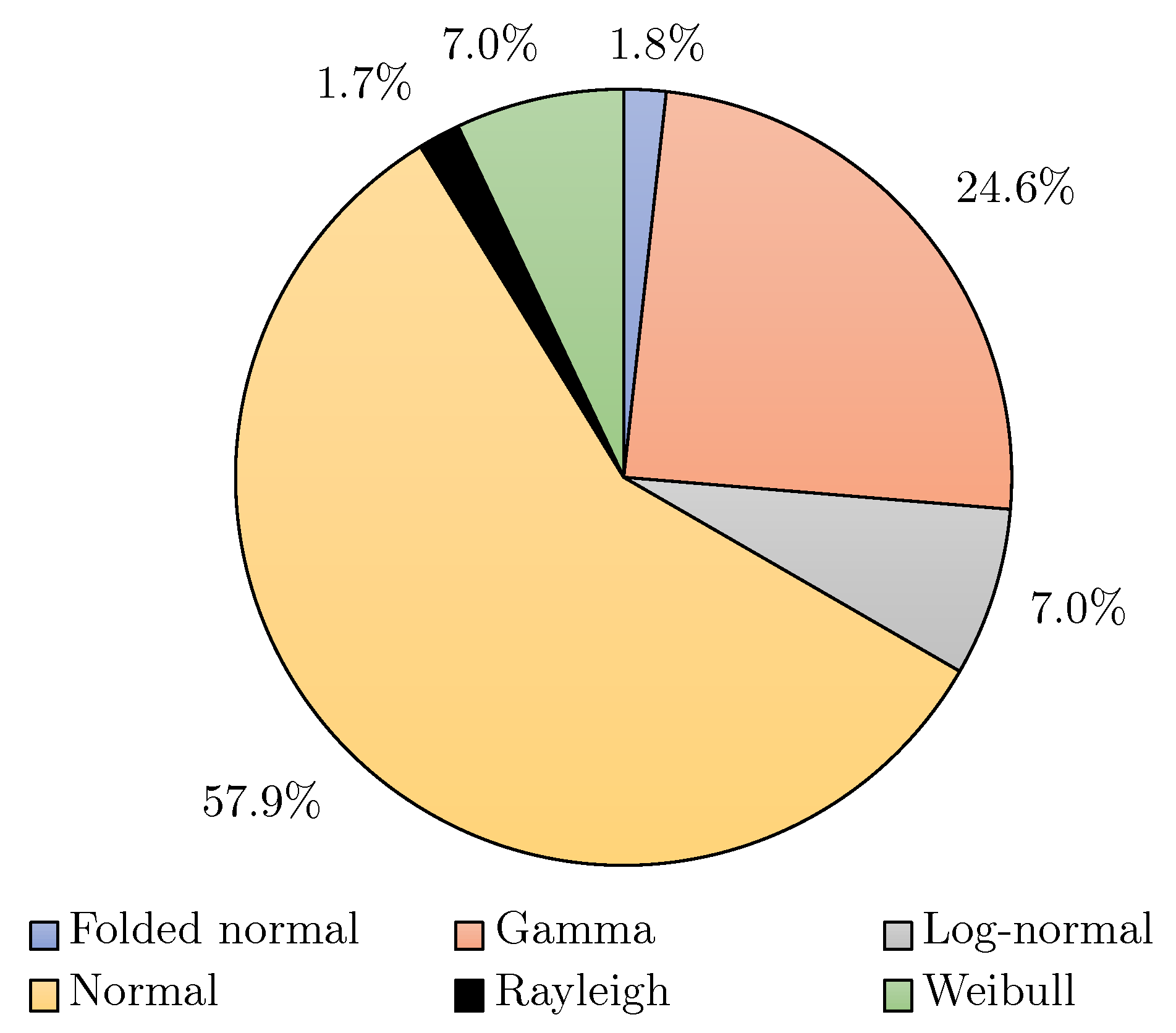
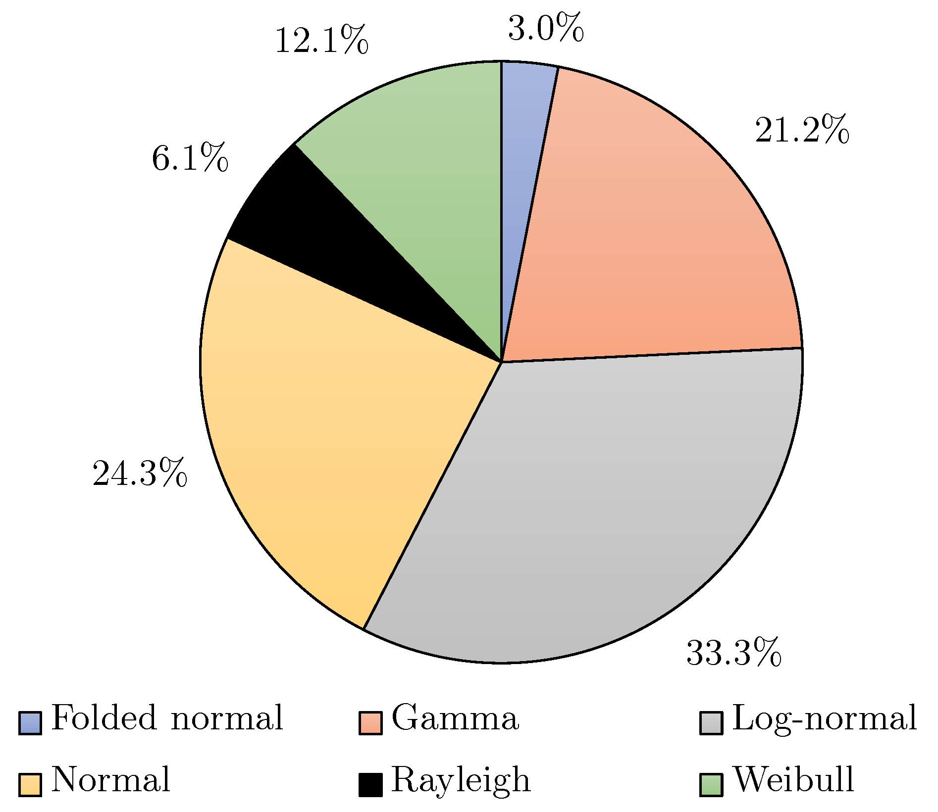
• Most of the dimensional measurements (57.9%) can be described using a normal distribution. The gamma distribution also fitted 24.6% of the measurements, while the log-normal fitted 7%. For the geometrical measurements, 33.3% best fitted a log-normal distribution, while 24.3% and 21.2% best fitted normal and gamma distributions, respectively. This is the first study to investigate the type of distribution that best fits the data.
• The method and GBTA design allowed the ISO 286-1 size ranges from 1 mm to 250 mm for the dimensional measurements to be covered and the dimensional and geometrical machine performance (potential and real) to be assessed. In both cases, the conventional target for $P_m$ and $P_{mk}$ indices of 1.67 (less than one part per million out-of-specification parts with a 95% confidence level) could be challenged. Indeed, depending on the final application of the parts, this index could be lowered to one (2600 rejected parts per million).
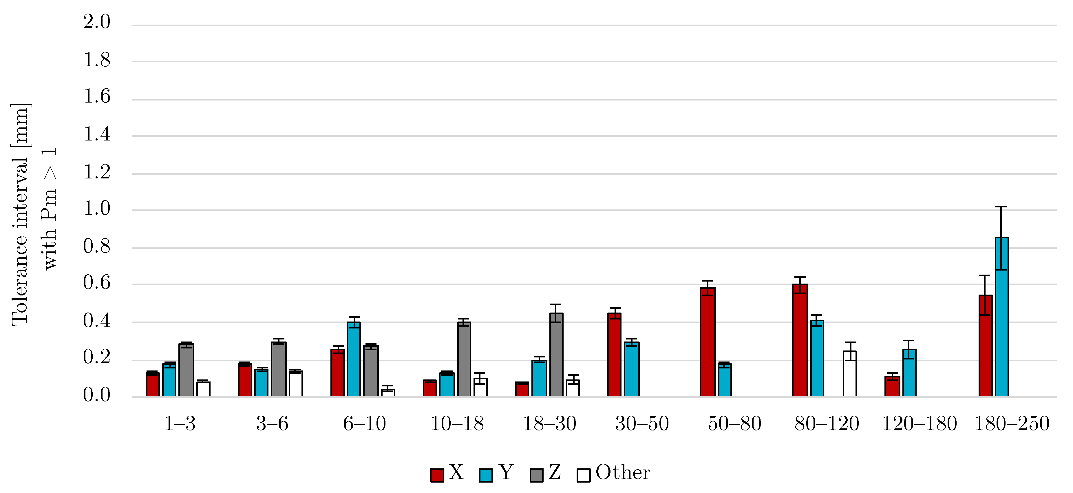
• The X and Y axes of the printer performed better than the Z axis, both for the potential and real machine performance. This allowed narrower tolerance intervals for the X and Y axes to be achieved, while ensuring the capable behavior of the printer.
• Both dimensional and geometrical results were sensitive to the design of the measured features as well as the printing conditions (especially layer height, which creates the potential staircase effect). Before foreseeing the fittings using the determined tolerance intervals, the designer should be careful. In some cases, it will be necessary to design a modified version of the GBTA to best take into account the type of geometrical features to be produced.
• Real machine performance $P_{mk}$ should be considered instead of using only the potential $P_m$. Indeed, as demonstrated, there can be a shift (systematic error) with respect to the middle of the desired tolerance intervals. Software compensation could solve this issue during the design process.
• A total of 27 h was required to print one part. Since 25 were needed, this may hamper the use of this GBTA design for industrial purposes and process monitoring. However, the proposed method is suitable for research and development purposes when assessing a new printer before market launch. Moreover, the method is systematic and provides a framework for assessing the machine performance of material extrusion printers.

References

1. ISO/ASTM 52900:2021; Additive Manufacturing General Principles Fundamentals and Vocabulary. ISO: Geneva, Switzerland, 2021.
2. Bourell, D.L.; Beaman, J.J.; Wohlers, T. History and Evolution of Additive Manufacturing. In Additive Manufacturing Processes; Bourell, D.L., Frazier, W., Kuhn, H., Seifi, M., Eds.; ASM International: Cleveland, OH, USA, 2020; pp. 11–18. [Google Scholar] [CrossRef]
3. Bourell, D.L.; Wohlers, T. Introduction to Additive Manufacturing. In Additive Manufacturing Processes; Bourell, D.L., Frazier, W., Kuhn, H., Seifi, M., Eds.; ASM International: Cleveland, OH, USA, 2020; pp. 3–10. [Google Scholar] [CrossRef]
4. Cruz Sanchez, F.A.; Boudaoud, H.; Camargo, M.; Pearce, J.M. Plastic recycling in additive manufacturing: A systematic literature review and opportunities for the circular economy. J. Clean. Prod. 2020, 264, 121602. [Google Scholar] [CrossRef]
5. SmarTech Analysis. Ceramics Additive Manufacturing Markets 2017–2028, an Opportunity Analysis and Ten-Year Market Forecast; Technical Report; Research and Markets: Dublin, Ireland, 27 September 2018. [Google Scholar]
6. Altıparmak, S.C.; Yardley, V.A.; Shi, Z.; Lin, J. Extrusion-based additive manufacturing technologies: State of the art and future perspectives. J. Manuf. Process. 2022, 83, 607–636. [Google Scholar] [CrossRef]
7. Gibson, I.; Rosen, D.; Stucker, B.; Khorasani, M. Additive Manufacturing Technologies; Springer International Publishing: Cham, Switzerland, 2021. [Google Scholar] [CrossRef]
8. Golhin, A.P.; Tonello, R.; Frisvad, J.R.; Grammatikos, S.; Strandlie, A. Surface roughness of as-printed polymers: A comprehensive review. Int. J. Adv. Manuf. Technol. 2023, 127, 987–1043. [Google Scholar] [CrossRef]
9. Kellens, K.; Mertens, R.; Paraskevas, D.; Dewulf, W.; Duflou, J.R. Environmental Impact of Additive Manufacturing Processes: Does AM Contribute to a More Sustainable Way of Part Manufacturing? Procedia CIRP 2017, 61, 582–587. [Google Scholar] [CrossRef]
10. Kara, S.; Li, W. Unit process energy consumption models for material removal processes. CIRP Ann. 2011, 60, 37–40. [Google Scholar] [CrossRef]
11. Leach, R.; Bourell, D.; Carmignato, S.; Donmez, A.; Senin, N.; Dewulf, W. Geometrical metrology for metal additive manufacturing. CIRP Ann. 2019, 68, 677–700. [Google Scholar] [CrossRef]
12. de Pastre, M.A.; Toguem Tagne, S.C.; Anwer, N. Test artefacts for additive manufacturing: A design methodology review. CIRP J. Manuf. Sci. Technol. 2020, 31, 14–24. [Google Scholar] [CrossRef]
13. Beltrán, N.; Álvarez, B.J.; Blanco, D.; Noriega, Á.; Fernández, P. Estimation and Improvement of the Achievable Tolerance Interval in Material Extrusion Additive Manufacturing through a Multi-State Machine Performance Perspective. Appl. Sci. 2021, 11, 5325. [Google Scholar] [CrossRef]
14. Flynn, J.M.; Shokrani, A.; Newman, S.T.; Dhokia, V. Hybrid additive and subtractive machine tools - Research and industrial developments. Int. J. Mach. Tools Manuf. 2016, 101, 79–101. [Google Scholar] [CrossRef]
15. Dantan, J.Y.; Huang, Z.; Goka, E.; Homri, L.; Etienne, A.; Bonnet, N.; Rivette, M. Geometrical variations management for additive manufactured product. CIRP Ann. 2017, 66, 161–164. [Google Scholar] [CrossRef]
16. Lussenburg, K.; Sakes, A.; Breedveld, P. Design of non-assembly mechanisms: A state-of-the-art review. Addit. Manuf. 2021, 39, 101846. [Google Scholar] [CrossRef]
17. Mavroidis, C.; DeLaurentis, K.J.; Won, J.; Alam, M. Fabrication of Non-Assembly Mechanisms and Robotic Systems Using Rapid Prototyping. J. Mech. Des. 2001, 123, 516–524. [Google Scholar] [CrossRef]
18. Minetola, P.; Calignano, F.; Galati, M. Comparing geometric tolerance capabilities of additive manufacturing systems for polymers. Addit. Manuf. 2020, 32, 101103. [Google Scholar] [CrossRef]
19. ISO/ASTM 52902:2023; Additive Manufacturing Test Artefacts Geometric Capability Assessment of Additive Manufacturing Systems. ISO: Geneva, Switzerland, 2023.
20. Spitaels, L.; Rivière-Lorphèvre, E.; Demarbaix, A.; Ducobu, F. Adaptive benchmarking design for additive manufacturing processes. Meas. Sci. Technol. 2022, 33, 064003. [Google Scholar] [CrossRef]
21. Lopes, A.J.; Perez, M.A.; Espalin, D.; Wicker, R.B. Comparison of ranking models to evaluate desktop 3D printers in a growing market. Addit. Manuf. 2020, 35, 101291. [Google Scholar] [CrossRef]
22. Vora, H.D.; Sanyal, S. A comprehensive review: Metrology in additive manufacturing and 3D printing technology. Prog. Addit. Manuf. 2020, 5, 319–353. [Google Scholar] [CrossRef]
23. Liu, Y.; Pears, N.; Rosin, P.L.; Huber, P. (Eds.) 3D Imaging, Analysis and Applications; Springer International Publishing: Cham, Switzerland, 2020. [Google Scholar] [CrossRef]
24. Rivas Santos, V.M.; Thompson, A.; Sims-Waterhouse, D.; Maskery, I.; Woolliams, P.; Leach, R. Design and characterisation of an additive manufacturing benchmarking artefact following a design-for-metrology approach. Addit. Manuf. 2020, 32, 100964. [Google Scholar] [CrossRef]
25. ISO 286-1:1988; Geometrical Product Specifications (GPS)—ISO System of Limits and Fits—Part 1: Bases of Tolerances, Deviations and Fits. ISO: Geneva, Switzerland, 1988.
26. ISO 2768-2:1989; General Tolerances—Part 2: Geometrical Tolerances for Features without Individual Tolerance Indications. ISO: Geneva, Switzerland, 1989.
27. ISO 17296-3:2014; Additive Manufacturing—General Principles—Part 3: Main Characteristics and Corresponding Test Methods. ISO: Geneva, Switzerland, 2014.
28. Juran, J.M.; Godfrey, A.B. (Eds.) Juran’s Quality Handbook, 5th ed.; McGraw Hill: New York, NY, USA, 1999. [Google Scholar]
29. Kane, V.E. Process Capability Indices. J. Qual. Technol. 1986, 18, 41–52. [Google Scholar] [CrossRef]
30. Kotz, S.; Johnson, N.L. Process Capability Indices—A Review, 1992–2000. J. Qual. Technol. 2002, 34, 2–19. [Google Scholar] [CrossRef]
31. Yum, B.J.; Kim, K.W. A bibliography of the literature on process capability indices: 2000–2009. Qual. Reliab. Eng. Int. 2011, 27, 251–268. [Google Scholar] [CrossRef]
32. Yum, B. A bibliography of the literature on process capability indices (PCIs): 2010–2021, Part I: Books, review/overview papers, and univariate PCI-related papers. Qual. Reliab. Eng. Int. 2023, 39, 1413–1438. [Google Scholar] [CrossRef]
33. ISO 22514:2016; Statistical Methods in Process Management—Capability and Performance. ISO: Geneva, Switzerland, 2016.
34. GmbH, R.B. Booklet No. 9 Machine and Process Capability. In Quality Management in the Bosch Group Technical Statistics, Bosch Group, Stuttgart Germany; Robert Bosch GmbH: Stuttgart, Germany, 2019; Volume 9. [Google Scholar]
35. Bissell, A.F. How Reliable is Your Capability Index? Appl. Stat. 1990, 39, 331. [Google Scholar] [CrossRef]
36. Chou, Y.M.; Owen, D.B.; Salvador, A.; Borrego, A. Lower Confidence Limits on Process Capability Indices. J. Qual. Technol. 1990, 22, 223–229. [Google Scholar] [CrossRef]
37. Montgomery, D. Introduction to Statistical Quality Control, 6th ed.; John Wiley & Sons, Incorporated: Hoboken, NJ, USA, 2008. [Google Scholar]
38. Kampker, A.; Kreiskother, K.; Buning, M.K.; Treichel, P.; Theelen, J. Automotive quality requirements and process capability in the production of electric motors. In Proceedings of the 2017 7th International Electric Drives Production Conference (EDPC), Würzburg, Germany, 5–6 December 2017; pp. 1–8. [Google Scholar] [CrossRef]
39. Volvo Group. Supplier Quality Assurance Manual; Volvo Group: Gothenburg, Sweden, 2019. [Google Scholar]
40. Safran. S_0002W_QA—Supplier Quality Assurance Requirements; Safran: Paris, France, 2023. [Google Scholar]
41. Safran. OP-741-02—Quality Requirements Applicable to Suppliers; Safran: Paris, France, 2020. [Google Scholar]
42. Maurer, O.; Herter, F.; Bähre, D. Tolerancing the laser powder bed fusion process based on machine capability measures with the aim of process control. J. Manuf. Process. 2022, 80, 659–665. [Google Scholar] [CrossRef]
43. Zongo, F.; Tahan, A.; Aidibe, A.; Brailovski, V. Intra- and Inter-Repeatability of Profile Deviations of an AlSi10Mg Tooling Component Manufactured by Laser Powder Bed Fusion. J. Manuf. Mater. Process. 2018, 2, 56. [Google Scholar] [CrossRef]
44. Günay, E.E.; Velineni, A.; Park, K.; Okudan Kremer, G.E. An Investigation on Process Capability Analysis for Fused Filament Fabrication. Int. J. Precis. Eng. Manuf. 2020, 21, 759–774. [Google Scholar] [CrossRef]
45. Preißler, M.; Rosenberger, M.; Notni, G. An Investigation for Process Capability in Additive Manufacturing; Universitätsbibliothek Ilmenau: Ilmenau, Germany, 2017. [Google Scholar]
46. Singh, R. Process capability study of polyjet printing for plastic components. J. Mech. Sci. Technol. 2011, 25, 1011–1015. [Google Scholar] [CrossRef]
47. Siraj, I.; Bharti, P.S. Process capability analysis of a 3D printing process. J. Interdiscip. Math. 2020, 23, 175–189. [Google Scholar] [CrossRef]
48. Udroiu, R.; Braga, I.C. System Performance and Process Capability in Additive Manufacturing: Quality Control for Polymer Jetting. Polymers 2020, 12, 1292. [Google Scholar] [CrossRef]
49. Yap, Y.L.; Wang, C.; Sing, S.L.; Dikshit, V.; Yeong, W.Y.; Wei, J. Material jetting additive manufacturing: An experimental study using designed metrological benchmarks. Precis. Eng. 2017, 50, 275–285. [Google Scholar] [CrossRef]
50. Dolimont, A.; Michotte, S.; Lorphèvre, E.R.; Ducobu, F.; Formanoir, C.D.; Godet, S.; Filippi, E. Characterisation of electron beam melting process on Ti6Al4V in order to guide finishing operation. Int. J. Rapid Manuf. 2015, 5, 320. [Google Scholar] [CrossRef]
51. Rebaioli, L.; Fassi, I. A review on benchmark artifacts for evaluating the geometrical performance of additive manufacturing processes. Int. J. Adv. Manuf. Technol. 2017, 93, 2571–2598. [Google Scholar] [CrossRef]
52. Bourdet, P. Logiciels des machines à mesurer tridimensionnelles. Techniques de L’ingénieur Mesures Mécaniques et Dimensionnelles Editions T.I. 1999; base documentaire: TIP673WEB. [Google Scholar] [CrossRef]
53. McGregor, D.J.; Rylowicz, S.; Brenzel, A.; Baker, D.; Wood, C.; Pick, D.; Deutchman, H.; Shao, C.; Tawfick, S.; King, W.P. Analyzing part accuracy and sources of variability for additively manufactured lattice parts made on multiple printers. Addit. Manuf. 2021, 40, 101924. [Google Scholar] [CrossRef]
54. Huang, Q.; Nouri, H.; Xu, K.; Chen, Y.; Sosina, S.; Dasgupta, T. Statistical Predictive Modeling and Compensation of Geometric Deviations of Three-Dimensional Printed Products. J. Manuf. Sci. Eng. 2014, 136, 061008. [Google Scholar] [CrossRef]
55. Baturynska, I. Statistical analysis of dimensional accuracy in additive manufacturing considering STL model properties. Int. J. Adv. Manuf. Technol. 2018, 97, 2835–2849. [Google Scholar] [CrossRef]
56. Cohen, D.L.; Lipson, H. Geometric feedback control of discrete-deposition SFF systems. Rapid Prototyp. J. 2010, 16, 377–393. [Google Scholar] [CrossRef]
57. Dou, C.; Elkins, D.; Kong, Z.J.; Liu, C. Online Monitoring and Control of Polymer Additive Manufacturing Processes. In Additive Manufacturing Design and Applications; Seifi, M., Bourell, D.L., Frazier, W., Kuhn, H., Eds.; ASM International: Cleveland, OH, USA, 2023; pp. 1–13. [Google Scholar] [CrossRef]
58. Bernard, A.; Kruth, J.P.; Cao, J.; Lanza, G.; Bruschi, S.; Merklein, M.; Vaneker, T.; Schmidt, M.; Sutherland, J.W.; Donmez, A.; et al. Vision on metal additive manufacturing: Developments, challenges and future trends. CIRP J. Manuf. Sci. Technol. 2023, 47, 18–58. [Google Scholar] [CrossRef]
59. Papazetis, G.; Vosniakos, G.C. Feature-based process parameter variation in continuous paths to improve dimensional accuracy in three-dimensional printing via material extrusion. Proc. Inst. Mech. Eng. Part B J. Eng. Manuf. 2019, 233, 2241–2250. [Google Scholar] [CrossRef]
60. Papazetis, G.; Vosniakos, G.C. Improving deposition quality at higher rates in material extrusion additive manufacturing. Int. J. Adv. Manuf. Technol. 2020, 111, 1221–1235. [Google Scholar] [CrossRef]
Figure 1. General distribution of measurements with the X 0.135 % , X 50 % , and X 99.865 % percentiles and the lower (L) and upper (U) tolerance bounds for a normal distribution.
Jmmp 08 00036 g001
Figure 2. Capable process (left, P m = P m k ) and shifted process (right, P m is >1 while P m k is <1) for normal distributions.
Jmmp 08 00036 g002
Figure 3. GBTA design used in this study.
Jmmp 08 00036 g003
Figure 4. Fitting of 600 Y-axis measurements from 3 mm to 6 mm with a Weibull distribution.
Jmmp 08 00036 g004
Figure 5. Type of distributions fitting the datasets for the dimensional measurements.
Jmmp 08 00036 g005
Figure 6. Type of distributions fitting the datasets for the geometrical measurements.
Jmmp 08 00036 g006
Figure 7. Dimensional tolerance intervals in mm with P m = 1.67.
Jmmp 08 00036 g007
Figure 8. Dimensional tolerance intervals in mm with P m = 1.
Jmmp 08 00036 g008
Figure 9. GBTA top surface (in green); Z measurements from 10 mm to 30 mm (in blue).
Jmmp 08 00036 g009
Figure 10. The 4 mm diameter bores of the GBTA for the X− (orange), X+ (grey), Y− (yellow), ad Y+ (blue) zones, and center 10 mm diameter bore (green).
Jmmp 08 00036 g010
Figure 11. Relative deviation in mm from the nominal value of the diameter of the GBTA bores for the Y−, Y+, X−, X+, and center zones.
Jmmp 08 00036 g011
Figure 12. Planes with dimensions between 50 mm and 80 mm combining several axes ((a), in green) and staircase effect of top hemispheres (b,c).
Jmmp 08 00036 g012