1. Introduction
Quenching steel workpieces is a heat treatment that includes heating the alloy at temperatures above 800 °C to form the austenite phase, followed by fast cooling to form the martensite phase. During quenching, fast cooling triggers the solid-state phase transformation. Failure to control either the magnitude or the distribution of the cooling rate in the workpiece may result in non-uniform phase transformation and thermal stresses leading to workpiece distortion and/or crack formation. Therefore, quantitative knowledge of temperature evolution during quenching becomes an essential step in designing new quenching systems, diagnosing quality-related problems, and finding solutions to improve productivity.
Convective flow boiling modeling for production lines requires efficient methods to approach complex phenomena, such as turbulent fluid flow and thermal radiation, combined with variable workpiece size and complex geometry. A recent comprehensive review of computational studies on boiling and condensation [
1] shows the current knowledge of convective flow boiling modeling. The authors acknowledge that computer modeling of single-phase convection has been tremendously successful for a wide variety of configurations, while modeling convective flow boiling has been limited mostly to simple configurations. Nevertheless, in their review, they did not include works regarding the role of heat conduction in a workpiece in the boiling and condensation processes. It is then fair to say that the number/scope of numerical studies on coupled heat conduction with convective flow boiling are considerably more limited than the convective flow boiling modeling reports.
Key studies that are relevant to the present work are summarized in
Table 1 and
Table 2.
Table 1 presents validation methods and remarks on models based on the interpenetrated phase equations. In this approach, vapor and liquid are well mixed in every computational cell. Therefore, the volume fraction of each phase is a continuous function of position. Kopun et al. [
2] simulated two routes of immersion quenching for a cast aluminum step plate with variable-thickness sections at different water pool temperatures. Their Eulerian multi-fluid model considered laminar flow and included additional interfacial forces such as lift and wall lubrication to ensure the drifting of the bubbles just away from the wall while essentially not affecting the phase distribution away from the wall. The heat flux continuity at the wall was represented by the following equation:
where
ks is the thermal conductivity of the solid workpiece,
n is the normal direction to the wall,
hw and
Tw are the heat transfer coefficient and wall temperature, respectively, and
Tsat is the saturation or boiling temperature. In their work, the heat transfer coefficient was estimated for each boiling regime: stable vapor film and transition boiling (the authors call it transition boiling, but it should be nucleation boiling, as explained above). The limit between these regimes is the Leidenfrost temperature, which was computed using empirical correlations implemented in the AVL FIRE
® CFD program and used to solve the corresponding differential equations. To improve the results, the authors proposed a variable Leidenfrost temperature, which may depend on the pool temperature, dipping velocity of the heated workpiece, immersion route, geometry of the workpiece, and wall surface roughness. Particularly, the authors derived an expression for the Leidenfrost temperature as a function of vertical position along the surface of the workpiece. The rates of vaporization/condensation of water were computed using semi-empirical equations that assume that the heat flux is proportional to the mass flux (between vapor and liquid). The model validation included a comparison between computed and measured cooling curves obtained from sub-superficial thermocouples installed in the workpiece. Sometime later, Zhang et al. [
3] presented an application of the previous model for immersion quenching of a cylinder head. Although there was a good agreement between computed and measured cooling curves, their results and conclusions reflect uncertainty in predicting the Leidenfrost temperature. Srinivasan et al. [
4] presented a numerical study of the immersion quench cooling process of a metallic trapezoidal block using the same Eulerian multi-fluid approach implemented in the AVL-FIRE
® v8.6 software. Their assumptions and the applied empirical and semi-empirical equations were very similar to those used by Kopun et al. [
2]. However, two differences should be pointed out. First, the solution method for coupling heat conduction in the solid with convection boiling. The authors used the AVL-Code-Couple-Interface (ACCI), which basically solves first the convection boiling under an isothermal solid wall and then the heat conduction in the solid under a constant heat transfer coefficient. This calculation process is repeated a few times to update both the wall temperature and heat transfer coefficient before moving on to the next step. This procedure has the advantage of accepting mutually independent meshes in solids and fluids. In contrast, Kopun et al. [
2] used the Multi-Material Approach (MMAT), which considers both solid and fluid as a single domain. Therefore, a single, whole solution is computed at every step. A second difference between these works is the Leidenfrost temperature. Srinivasan et al. [
4] considered that Leidenfrost temperature did not depend on position on the workpiece surface. Model validation was carried out by comparing computed and measured cooling curves. Another numerical simulation of flow-boiling heat transfer was presented by Krause et al. [
5]. Their model also belongs to the interpenetrated phases category; however, there are some differences with respect to the previously described works. First, they used the mixed model, which solves the continuity and momentum equations for the mixture of vapor and liquid rather than solving these equations individually for each phase. Further, average properties are weighted on volume fractions and phase densities rather than exclusively volume fractions. Moreover, the vaporization/condensation rates are computed from the mass source/sink terms in the continuity equation using the bubble crowding model. This model only establishes that the rate of phase transformation is proportional to the super-heating or under-heating of the fluid with respect to the boiling temperature,
Tsat. The coefficient of proportionality depends on the local mass transfer coefficient, which in turn is a function of the boiling regime, the temperature at the critical heat flux,
Tcrit, and the Leidenfrost temperature,
TL. Therefore, there is no need for a priori knowledge of nucleation site density or a vapor-liquid interphase to start boiling. The authors supported this assumption by recalling that workpiece surfaces are technically rough and liquids are not pure, resulting in a great number of nucleation/condensation sites. The authors implemented their model in the CFD Fluent 6.3 code to compute iteratively the mass transfer coefficient by assuming a starting value of 1 m/s and minimizing the difference between their computed heat transfer coefficient and the corresponding measured values. Model validation was based on comparing calculations with experimental results for two cases: a steady-state case using an isothermal metallic cylinder immersed in a vertical tube where water was flowing at an average velocity of 0.3 m/s. In this case, validation was based on a qualitative comparison between computed and observed bubble fractions at the half height of the vertical cylinder that was held at 400, 500, and 1000 K. The second case was a transient heat transfer during the quenching of the same cylinder. Validation was based on a comparison between computed and experimentally determined heat transfer coefficients. Notice that the mass transfer coefficient at the vapor-liquid interphase was determined using this experimental heat transfer coefficient. Stark et al. [
6] presented a numerical study of the quenching process using a confined water jet. The liquid velocities at the nozzle were 1 or 3 m/s, and the distances from the nozzle to the austenitic steel wall were 50 or 100 mm, respectively. They simulated steady-state convection boiling, assuming an isothermal wall. The wall temperatures had different values between 300 and 900 °C; therefore, all the boiling regimes were analyzed. The computed heat transfer coefficients as a function of wall position and temperature were used in a separate calculation to solve the heat conduction equation for the solid plate. Therefore, they decoupled heat conduction in the solid from convective boiling. Regarding convective boiling, it was computed using a mixed model, like Krause et al.’s model, and the interaction between liquid and vapor “bubbles” was defined using the Schiller–Naumann correlation for momentum exchange and the Ranz-Marshall correlation for heat transfer. The required bubble diameter for these correlations was a linear function of the vapor fraction. Turbulent flow was considered using the
k-
w-SST (Shear Stress Transport) model. Sinks and sources, included in the conservation equations, expressed the rate of phase change from boiling/condensation. The model was implemented in the CFD package, Ansys Fluent
® 13. The authors claimed that their single model approach allows for the investigation of all occurring boiling phases during the quenching process, avoiding specifying in advance the temperature range where each boiling regime is present. However, the authors did not present a model validation by comparing their numerical results against experimental measurements. Passarella et al. [
7] developed another multiphase mixed model to simulate the quenching of a low-carbon steel cylinder using mineral oil flowing in a vertical tube at 1 m/s. The momentum equation was solved under turbulent conditions using the
k-
e model implemented in the Comsol
® Multiphysics code.
The interaction between vapor bubbles and liquid was computed using a drift flux mixture model. Liquid heat flux conduction at the wall and wall shear stress were computed using adequate wall functions. Additionally, they assumed that the total heat conduction from the solid was equal to the sum of the heat that increased the liquid temperature plus the heat used to evaporate this fluid. Also, it was considered that the vapor temperature was not raised above
Tsat to avoid solving the energy equation for this phase. The proportion of heat for each contribution determined the boiling regime that was present. This proportion was controlled by damping functions: one depending on wall temperature,
fT, and another on vapor fraction,
fv. Different empirical and semi-empirical expressions were used for the heat flux under the stable vapor film regime and for the nucleation boiling regime. The authors showed the computed evolution of the vapor fraction and solid temperature. The vapor-rich layer starts in two zones: the upper area and the lower area of the cylinder surface. Then, it moves towards the mid-height of the cylinder. Despite the authors claiming the correctness of these results, no experimental evidence was shown in the article to support their calculations on the vapor fraction distribution. Nevertheless, the authors obtained computed heat transfer coefficient values with the same order of magnitude as previous experimentally determined values. In a recent study, Petrovic and Stevanovic [
8] reported a coupled two-fluid flow and wall heat conduction modeling of nucleate pool boiling. Their model is also in the category of Eulerian multi-fluid with interpenetrated phases, solving numerically the mass and momentum differential equations for each phase: liquid and vapor. The energy equation for the liquid was coupled with the heat conduction equation for the solid workpiece. The interaction between liquid and vapor was given by an interfacial drag force per unit volume for momentum transfer and the rates of evaporation/condensation for mass transfer. The finite volume method [
9] was used to solve the conservation differential equations. In contrast with the previous works, the total wall heat flux was divided into two contributions: a convective heat flux and a vaporization heat flux. The former represents the heat flowing from the wall to a liquid film, while the second one represents the heat flowing to growing bubbles. This approach took several results from previous works regarding the dynamics of bubble growth, which required input data like nucleation site density and the wetting contact angle. The authors found that the computed boiling curve strongly depended on these input data. Model validation was carried out using data from steady-state experiments, where a heater was used to hold a time-independent temperature distribution in a steel plate immersed in still water. The authors compared the obtained relationship between computed wall heat flux and nucleation site density with the respective observed relationship reported by other authors. Also, the authors showed comparisons between observed and computed vapor fraction distributions and heat transfer coefficients along the height of the heater. Finally, using transient heat flow results, they compared their computed temperature profiles across a cold spot at the location of a bubble growth with the corresponding measured values reported previously. In this study, wall temperatures were always below 130 °C; therefore, a stable film boiling regime was not present.
Table 2 presents validation methods and remarks on interface-capturing-methods. This approach includes the calculation of the interphase position; therefore, the volume fraction of each phase in all computational cells is either 0 or 1, depending upon the location of the interphase. This method predicts a more detailed picture of the vapor-liquid distribution than the interpenetrated phases approach does. However, the computational cost is considerably higher. Ramezanzadeh et al. [
10] used the Volume-Of-Fluid (VOF) method to compute the temperature evolution in a steel step plate subjected to quenching when immersed in oil flowing at constant velocities of 0.1, 0.2, 0.3, 0.5, or 0.6 m/s. The authors implemented a source term in the continuity equation to create a higher interface resolution between vapor and liquid. The continuous surface force model (CSF) was used to account for the effect of surface tension on the interface shape. The rates of vapor formation and condensation were computed using the Lee mass transfer model since it does not require an initial interface condition and boiling starts anywhere in the liquid if the temperature is higher than the saturation temperature. Validation was carried out in two steps. First, the authors used their model to calculate the one-dimensional Stephan boiling problem, and second, they compared the computed cooling curves against the corresponding measured values as reported by other authors. It is interesting to note that their calculations show the simultaneous presence of different boiling regimes in different zones of the workpiece surface. These numerical results led to an optimal oil velocity of 0.3 m/s to achieve a uniform workpiece temperature during cooling. However, no experimental observations supported this conclusion. Another work based on the VOF method was reported by Moon et al. [
11]. The authors reported a numerical study on a vertical water-free jet impinging on a superheated stainless-steel plate. The initial steel temperature was 900 °C, but they neglected radiation heat transfer and justified this assumption based on an initial fast cooling of the metallic surface. Boiling/condensation rates were calculated from the Lee model; therefore, no nucleation site density was required. Fluid flow near the wall was computed using the turbulent
k-
w SST model. The corresponding wall distance
y+ was set equal to 10 to properly calculate the turbulent viscosity. The nozzle was 3 mm in diameter and was located 100 mm from the plate surface. The circular plate was 100 mm in diameter and 60 mm thick. The water left the nozzle at 20 °C at a velocity such that the Reynolds number was 15,000. The authors compared the measured cooling curves for a location under the stagnation point with the corresponding model predictions, and they also compared the respective boiling curves. The authors computed a radial component of the temperature gradient in the plate that was larger than the axial component of the temperature gradient. This was attributed to the radial distribution of different boiling regimes on the wall, which led to quite different heat fluxes along the metallic surface. Single-phase convection was present at the stagnation point, and a stable vapor layer prevailed at some distance from the stagnation point. Zhang et al. [
12] studied the influence of wall thickness and thermal diffusivity on dynamics and heat transfer in the nucleate pool boiling of a single bubble. They used the Ghost Fluid Method for sharp interface representation. Two Level Set functions were used to capture the liquid-vapor and liquid-wall interfaces. The computational domain included an axisymmetric solid and a fluid on its upper face. The fluid region was divided into micro- and macro-regions. The momentum, energy, and continuity equations were solved considering laminar flow and constant physical properties. The heat conduction equation was solved for the solid wall, assuming that its lower face was isothermal. The authors found that the bubble growth time decreases with the wall thickness, but the departure bubble diameter increases. A local and periodic expanding-receding low-temperature region was produced inside the wall under the bubble base because of movement of the contact line (vapor-liquid-wall line) due to evaporation of the liquid microlayer. An increase in wall thermal diffusivity lags the movement of the local low-temperature region. The authors did not show any measurements or observations to validate their results. It is evident that this interface-capturing method offers the capability to compute, from first principles, macroscopic parameters used by multi-fluid interpenetrated models, for example, nucleation site density. A recent work by Cukrov et al. [
13] shows a model aimed at the stable vapor film regime using the VOF method. They considered the immersion quenching of a short cylinder in saturated still water at 600 °C. The authors used the energy jump mass transfer model to determine the evaporation rate. They claimed that this model does not require empirical input to estimate the mass transfer rate across the interface. The calculations agree with a previously measured cooling curve within the stable vapor film regime. The authors claim that this agreement shows an accurate calculation of the temperature gradient at the vapor-liquid interface in the mass transfer model and adequate turbulence modeling, although turbulence kinetic energy was considered uniform and constant. The authors, Ilic et al. [
14], presented a review and future prospects of boiling heat transfer modeling. They pointed out that, besides interpenetrated (macro-scale boiling) and interface-capturing (micro/meso-scale boiling) models, molecular dynamics (nano-scale boiling) methods represent an alternative to improve our understanding of boiling heat transfer mechanisms. These methods are based on computing the trajectories of individual molecules, which move according to the interacting forces. The author’s opinion is that the most important advantage of these methods is that the bubble nucleation site can be detected for different geometrical configurations and wettability conditions of the wall. According to the authors, multi-scale modeling is the future prospectus for an improved predictive methodology of boiling heat transfer phenomena. Multi-scale modeling is a combination of macro-scale, micro/meso-scale, and nano-scale models. However, the authors accept that there is no definite answer to the question of how these scales should be coupled with each other.
From the above literature review, it was identified that validation methods are not detailed enough to include information on both solid bodies and fluids, and generally they consider just one of them, either cooling curves or boiling characteristics. Also, there is no reported model, thoroughly validated, that includes both turbulent flow and thermal radiation, which are very common phenomena during metal quenching. Finally, only the recent work of Moon et al. [
11] reports the importance of observing simultaneous multi-regime boiling on the wall heat flux distribution. The present work presents an interpenetrated phase model that includes turbulent flow and thermal radiation and was validated using cooling curves and the advance of the wetting front along the solid wall. The model was used to determine the wall heat flux components, finding that simultaneous multi-regime boiling is an undesirable condition from the product quality point of view since it leads to non-uniform heat flux.
Because of the approach taken, the model is computationally efficient, despite including turbulent flow and thermal radiation calculations. Therefore, this model is suitable for quenching simulations of larger and more complex workpieces.
Table 2.
Interphase-capturing-models, validation methods, and remarks.
Table 2.
Interphase-capturing-models, validation methods, and remarks.
| Author, Year | Model Validation | Remarks |
|---|
| Ramezanzadeh et al. (2017) [10] | Cooling curves in the workpiece | Volume Of Fluid method. No radiation, Tw < 627 °C (900 K), laminar flow (Re ≤ 1770). Calculation of simultaneous different boiling regimes on the wall. |
| Moon et al. (2022) [11] | Cooling curves and boiling curves | Volume Of Fluid method. No radiation; Tw ≤ 900 °C. Turbulent flow, Renozzle = 15,000, k-w SST model. Calculation of simultaneous different boiling regimes on the wall. |
| Zhang et al. (2015) [12] | No validation with experimental results | Level Set method was applied twice: for the vapor-liquid interface and for the liquid-wall interface. Gosh Fluid Method for a computed sharp interface. No radiation; Tw ≤ 106 °C. Pool boiling, laminar flow. |
| Cukrov et al. (2023) [13] | Cooling curve and qualitative shape of the vapor bubble column | Volume Of Fluid method. No radiation, Tw ≤ 600 °C. Turbulent flow, k = 0.25 m2/s2. Stable vapor film regime |
3. Mathematical Model
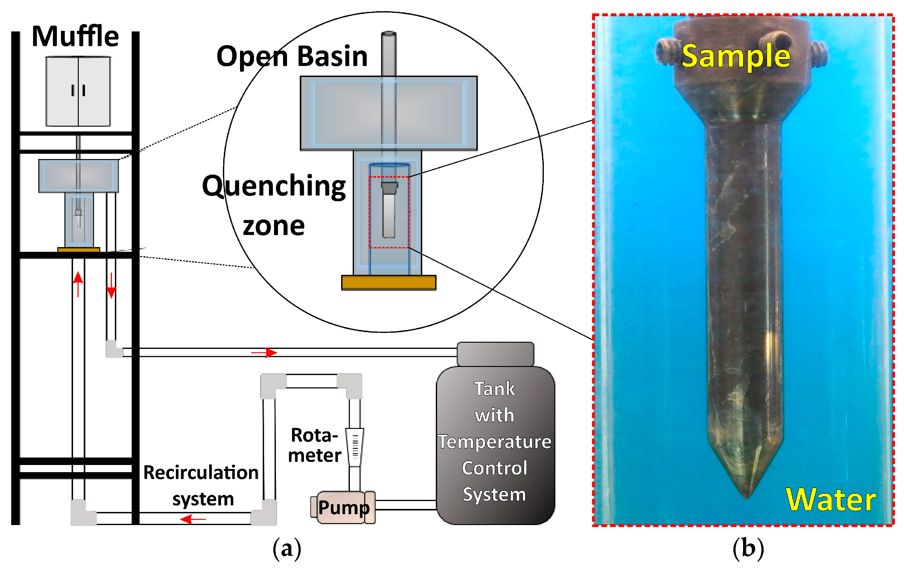
Before presenting the model equations, it is convenient to review the following considerations: The probe was heated up in a muffle until it reached a uniform temperature. Then, this probe was taken out of the muffle and moved down in still air at a manually controlled velocity. During this period, the probe was cooled down by natural convection and radiation, which led to Newtonian cooling (Bi < 0.1). Therefore, the probe temperature was essentially uniform, and there was no need to solve the heat conduction equation for the probe. However, after immersion started, at t = 0, the sample surface was covered quickly by the flowing water, increasing the heat flux at the wall and leading to non-Newtonian cooling (Bi > 0.1). Vapor forms on the probe surface, leading to a heat transfer coefficient that evolves as a function of the wall temperature and fluid flow conditions. Also, radiation absorption by liquid water and vapor took place. The present analysis of this process was carried out by coupling the solution of the fluid flow equations and the heat conduction equation for the solid probe.
Five phenomena were considered during the quenching process:
(1) The fluid dynamics of water; (2) the interfacial heat transfer between solid and fluid; (3) the heat losses from the probe surface by radiation; (4) the interfacial mass transfer between liquid and vapor phases during water boiling; and (5) the heat conduction through the solid probe.
The interaction between these phenomena was represented by the numerical solution of the following coupled differential equations.
3.1. Governing Differential Equations
3.1.1. Mixture Model
The mixture model was adopted for this work since the criteria of the Stokes number and the bubble loading are satisfied [
17]. The Stokes number (St) is defined as the ratio of the bubble response time to the system response time. Considering a constant bubble diameter of 0.1 mm [
18], the estimated order of magnitude of the Stokes number is 10
−6, which means that the vapor bubbles follow the water streamlines. The bubble loading is defined as the mass density ratio of vapor bubbles to that of the liquid water. Estimated orders of magnitude values considering vapor volume fractions of 0.05 and 0.95 are 10
−5 and 10
−2, respectively. This is a very low loading, so the coupling effect between phases is one-way, which means the water influences bubbles via drag and turbulence, but the bubbles have no effect on the water flow. On the other hand, the Eulerian interpenetrated phases models do not compute explicitly the interphase boundary, as opposed, for example, to the Level Set or the Volume of Fluid methods, which do track the actual position of the interphase boundary. However, in the mixture model, it is possible to specify an interphase position by conventionally setting a volume fraction value. For example, a vapor-liquid boundary can be defined as those points in space where the volume fraction of vapor is equal to 0.5. Complementary, notice that for pure water, the liquid volume fraction is one, and analogously for pure vapor. Therefore, the considered differential equations also apply for the single-phase regions.
The mixture model solves the continuity, momentum, and energy differential equations for the mixture and the conservation equation for the vapor phase (secondary phase) to compute the rate of evaporation/condensation. These equations are described as follows:
Continuity equation,
where
is the mass-averaged mixture velocity, and it is calculated by the following expression:
being subindex
k equal to 1 for liquid phase and 2 for vapor phase, and
is the mixture density, computed from the equation:
where
is the volume fraction of phase
k.
Momentum equation
where the present forces are the pressure gradient (
), gravitational force per unit volume of mixture (
), viscous forces that depend on the dynamic viscosity of the mixture
, computed from the following expression:
and the momentum transfer due to the relative velocity between phases, so called slip velocity, (
). This relative velocity is computed by using an algebraic slip formulation, which assumes that a local equilibrium between phases was reached over a short spatial length scale. Therefore, slip velocity could be expressed as a function of the vapor bubble acceleration and a drag function. In the present model, this drag function is from Schiller and Naumann [
19]:
where the Reynolds number,
Re, is computed using the slip velocity. On the other hand, the acceleration of bubbles is given by gravity force; therefore, the algebraic slip formulation leads to the so-called drift flux model. The drift velocity for phase
k is relative to the mixture velocity and is given by the following equation:
Energy equation
Considering incompressible flow and radiation absorption, the energy equation can be written as:
where
Hk is the sensible enthalpy for phase
k,
keff is the effective thermal conductivity, which is defined by the following equation:
being
kk the material thermal conductivity of phase
k, and
kt the turbulent thermal conductivity defined according to the used turbulence model. The heat source,
Sh, includes two terms: (1) the latent heat for evaporation/condensation, which was computed from the Lee model combined with the semi-mechanistic boiling model, and (2) the thermal radiation absorption, which was evaluated from the Discrete Ordinates (DO) radiation model. Both models are explained below.
3.1.2. Evaporation/Condensation Model
The calculation of the rate of interphase mass transfer through evaporation-condensation was carried out using the Lee model [
20], which is a mechanistic model based on the solution of the vapor conservation equation, written as follows:
where
and
are the rates of evaporation and condensation, respectively, and are given by the following equations.
where
cevap and
ccond are the evaporation and condensation coefficients, respectively, which are interpreted as the inverse of relaxation times, which must be fine-tuned to match experimental data for each system, and
T1 and
T2 are the local temperatures for liquid and vapor phases, respectively.
Regarding the wall heat flux, it was computed using the semi-mechanistic boiling model. This approach is particularly useful for low-pressure boiling systems, such as metal quenching. The semi-mechanistic model includes heat transfer augmentation at the wall due to boiling, which was computed from empirical correlations developed by Chen [
21]. The effective wall heat flux is expressed as the weighted sum of the nucleate boiling heat flux resultant of the micro-convective mechanism associated with bubble nucleation and growth and the forced convective heat flux associated with the macro-convective mechanism related to fluid flow. It is assumed that the convective and boiling contributions could be superimposed but need to be modified by the effects of vapor quality and the interaction between mechanisms. Because of that, this model assumes that vapor formed by the evaporation process increases the liquid velocity, and, therefore, the convective heat transfer contribution is augmented relative to that of a single-phase liquid flow. On the other hand, the convection partially suppresses the nucleation of boiling sites; thus, the contribution of nucleate boiling is reduced. These phenomena are represented by the following expression:
where
F is the forced convective augmentation factor,
S is the nucleate boiling suppression factor, and
Msp and
Mnb are the heat flux multipliers for the single phase and nucleate boiling, respectively. The first term on the right side of this equation represents the single-phase contribution, and the corresponding heat flux,
qsp, was calculated from the basic relationship for heat transfer by convection:
qsp =
hspΔ
T, where the single-phase heat transfer coefficient,
hsp, was obtained from the following equation.
being
h1 and
h2 single-phase heat transfer coefficients for liquid and vapor, respectively,
f is the area fraction of wall surface wetted by the liquid, and Δ
T is the difference between the wall and boundary cell temperatures (
Tw −
Tc). The factor
F is strictly a fluid flow parameter and is expressed as follows [
22]:
This factor is a function of the Martinelli parameter
Xtt, which is used to determine the influence of two-phase presence on convection, and it is calculated from the following expression:
where
χ is the local vapor mass fraction (vapor quality).
The second term on the right-hand side of Equation (13) represents the contribution of the nucleate boiling mechanism, and the respective heat flux,
qnb, was computed using the general equation
qnb = hnbΔ
Tsup. The corresponding heat transfer coefficient,
hnb, was calculated using the Foster and Zuber correlation, written as follows [
23],
being
Psat,Tw and
Psat,Tsat the saturation pressures corresponding to wall temperature and saturation temperature, respectively;
k1,
cp1,
ρ1, and
μ1 are the thermal conductivity, specific heat, density, and viscosity of the liquid, respectively;
ρ2 is the vapor density;
H12 is the latent heat of vaporization; and
γ is the surface tension of water. The superheat, Δ
Tsup, is equal to the difference
Tw −
Tsat.
The suppression factor,
S, is defined according to the following equation:
where
Ssub accounts for the subcooled effects, and it is calculated from the expression proposed by Steiner et al. [
24].
being
Tref a reference temperature.
Sfc represents the suppression factor due to forced convection, which can be found elsewhere [
22] and depends on the two-phase Reynolds number, according to the following expression.
The modified two-phase Reynolds number is defined as follows:
being the reference Reynolds number for liquid calculated as:
where,
are the density and viscosity of liquid, respectively, at the reference temperature.
is the reference velocity, and
L is the characteristic length scale.
It is convenient to note that Equations (11)–(22) allow for the computation of the full boiling curve, which includes the regimes of single-phase convection, nucleation boiling, and stable vapor film. Therefore, no extra Leidenfrost temperature model is required since Leidenfrost temperature is implicitly computed using those equations. However, in the present work, it was found that this model predicted, during the stable vapor film regime, probe temperatures that were essentially constant. Changing the coefficients of the evaporation and semi-mechanistic models did not change this result. Therefore, thermal radiation was included in the model since it is known that this heat transfer mechanism is particularly important during the stable vapor layer regime. Then, the cooling curves matched reasonably well from the beginning of the cooling process, as shown in
Section 4.2.
3.1.3. Thermal Radiation Model
Vapor and liquid water interact with the thermal radiation from the wall by absorbing, reflecting, and transmitting the received radiation in different proportions and emitting their own radiation. Additionally, wall surface properties such as emittance (ε) and absorptance (α) also play a role in determining the net heat flux from the surface. Nevertheless, most works on numerical simulation of heat treatment of metals neglect radiation heat flux, arguing that the period that the surface is at high temperatures is very short. This is misleading since the whole thermal history of the probe and the resulting microstructure and mechanical properties of the probe are dependent on its initial temperature and its initial cooling rate. From the available radiation models, the selection of the Discrete Ordinates (DO) method was based on the following advantages: (1) The DO model applies for systems that are optically thin, which is defined by an optical thickness value αL < 1, where α is the absorption coefficient of the fluid and L is the characteristic length scale of the domain; (2) it allows the solution of radiation in semi-transparent materials; and (3) the computational cost is moderate.
The DO model solves the Radiative Transfer Equation (RTE) for a finite number of discrete solid angles,
, each associated with a directional vector,
, fixed in the coordinate system. The RTE can be expressed as follows:
where
is the radiation intensity, which depends on position vector,
, and direction vector,
is the phase function which depends on the dot product between the direction vector and the scattering direction vector,
are the absorption coefficient, scattering coefficient, and refractive index of the medium, respectively;
is the Stefan–Boltzmann constant and
= 3.141592… Finally,
is the path length, and
T is the absolute temperature. The DO method consists of transforming Equation (23) into a transport equation for radiation intensity and solving for as many transport equations as there are directions
. The solution method is the same as that used for the fluid flow and energy equations.
The DO model allows the specification of an opaque wall adjacent to a fluid or solid zone; however, it is necessary to specify the opacity condition directly at the boundary. Furthermore, the steel surface was considered to diffusely reflect the incoming radiation from the fluid.
3.1.4. Turbulence Model
The turbulence model k-
ω SST was chosen to compute the interphase turbulence, where k is the turbulence kinetic energy and
w is the specific dissipation rate. This approach is better suited for wall-bounded flows than the classical k-
ε, RMS (Root Mean Square), or LES (Large Eddy Simulation) models, which are intended for turbulent core flows, i.e., regions that are far from walls. The k-
ω semi-empirical model was developed to be applied throughout the boundary layer, provided that the near-wall mesh resolution is sufficient. This standard model has been improved, leading to the k-
ω Base Line (BSL) and SST versions. Both versions can be used to describe near-wall and far-wall flows present in the same problem. However, the SST model accounts for the transport of the turbulence shear stress in the definition of turbulent viscosity. Therefore, the SST model is more accurate and reliable for a wider class of flows than the standard and BSL models. A full set of equations and constants for this model can be found elsewhere [
25].
3.1.5. Heat Conduction
The solid probe is the main source of energy in this system. Heat conduction takes place in the axial and radial directions. The heat conduction equation is a particular case of the previous energy equation since there is only a solid phase and no velocity. The heat conduction equation can be written as:
where subscript “
s” means solid phase.
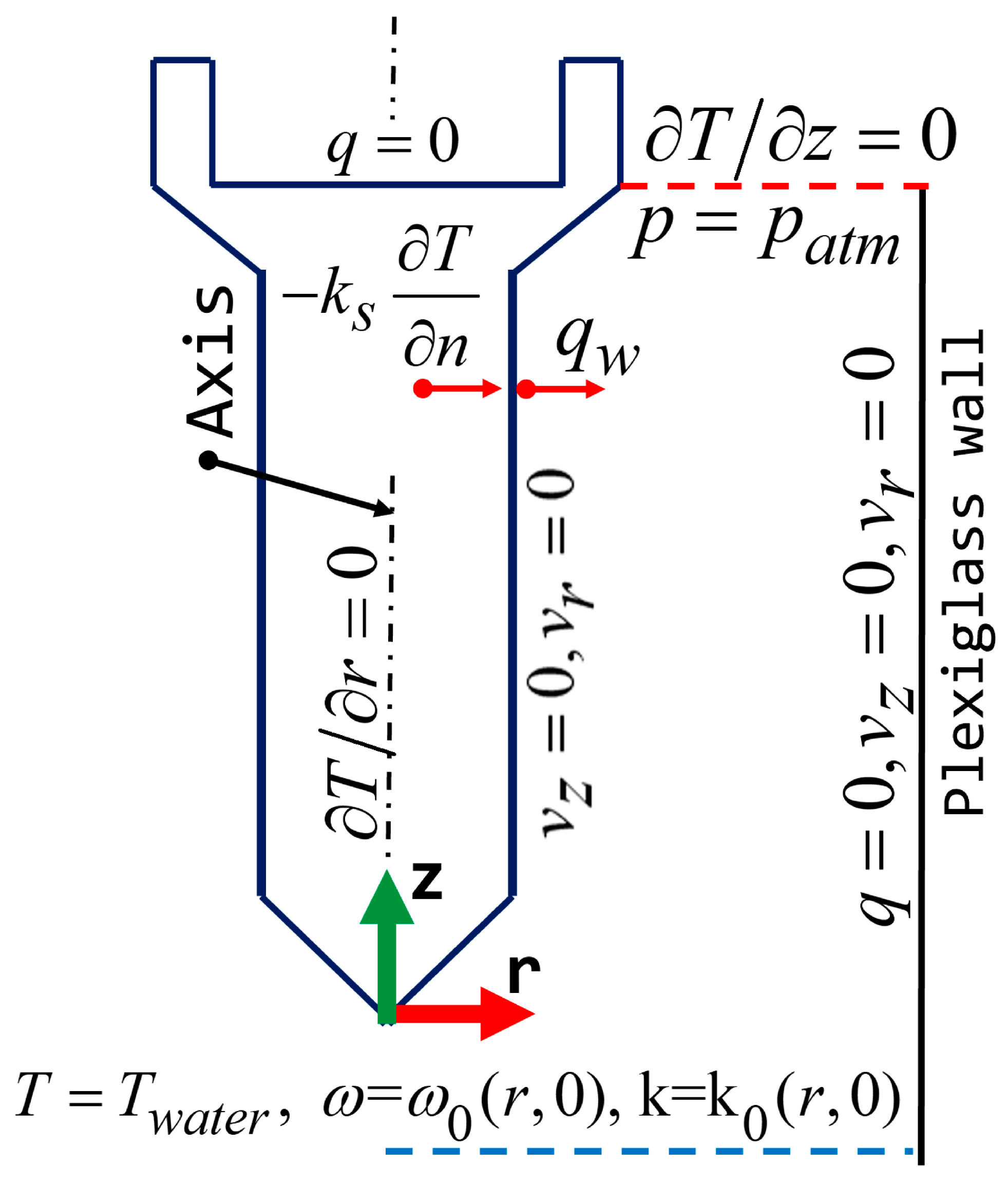
3.2. Initial, Boundary, and Internal Conditions
It is convenient to define several time points that characterize the quenching progress. These points are called “F”, “A”, “B”, “C”, “D” and “E” and are explained below. The initial time,
t = 0, corresponds to the point when the tip of the conical base of the probe just touched the water-free surface in the basin. At this point, the probe starts its immersion into the flowing water; this is point “F”. For modeling purposes, a representation of this process was adopted. It was assumed that at
t = 0, the whole probe was instantaneously immersed, and the steady water flow velocity was increased by adding the immersion velocity to it and increasing proportionally the turbulent kinetic energy of the water. This velocity increment was applied only to a couple of rows of boundary fluid cells, which were at distances < 2.8 mm from the wall. The size of boundary cells is 1.4 mm, which satisfies the convergence condition for the dimensionless position
y+ > 30 that grants inclusion of the viscous sublayer and the buffer layer. Notice that quenching modeling starts with the fully immersed probe that still corresponds to point “F” since
t = 0. The duration of this velocity increment was equal to the actual immersion time. After this short period, the probe is at point “A”.
Table 4 summarizes the initial conditions for the solved differential equations. The table shows that the initial water velocity field was computed previously in an independent calculation, assuming that the probe is already in its final position inside the vertical tube and that it is at water temperature. Therefore, the continuity, momentum, and turbulence equations were solved under steady-state and isothermal conditions. The initial pressure and turbulent quantities, k and
ω, correspond to this previous calculation. Finally, the probe temperature is uniform since the Biot number is smaller than 0.1 during air-cooling when transporting the probe from the muffle to the quenching position.
The boundary and internal conditions applied to solve the governing equations are graphically shown in
Figure 3. The axisymmetric domain included a water inlet surface, a water outlet surface, a symmetry axis, and the following solid boundaries: a Plexiglas tube wall and a probe top surface; and the internal boundary was the probe lateral surface.
Continuity, momentum, and turbulence equations require the following boundary conditions:
The profiles of inlet velocity and turbulent quantities were previously calculated and correspond to a fully turbulent, developed profile, v(r), since the inlet surface is far enough from the elbow connector located upstream and from the solid probe to avoid any flow distortion. At the outlet, a reference atmospheric pressure, patm, was specified. A zero-velocity wetting condition was specified over the tube surface and on the probe surface, and a near-wall treatment was used to specify turbulent quantities on those wall surfaces.
The energy equation requires specifying an inlet water temperature, an outlet zero temperature derivative in the axial direction, zero heat flux on the Plexiglas wall, zero heat flux on the probe top surface, and a near-wall treatment for turbulent heat flow in the probe wall surface.
The near-wall treatment accounts for the effect of the wall presence on the turbulence. The region that is closer to the wall has tangential velocity fluctuations that are reduced by viscous damping, while the normal velocity fluctuations are reduced by kinematic blocking. Outside of this zone, turbulence is rapidly augmented by the generation of turbulent kinetic energy. The limits of the viscous sublayer, the buffer layer, and the fully turbulent region are represented by the dimensionless distance from the wall,
y+, which is defined by the following equation:
where the friction velocity,
ut, is defined as
Being
τw the shear stress on the wall. A value
y+ < 30 represents a region that includes the viscous sublayer and the buffer layer. In the present approach, semi-empirical equations, called “wall functions”, were used to bridge the variables between the viscous sublayer and the fully turbulent region. Wall functions are used in meshes with
y+ > 30. Therefore, the first control volume next to the wall will include the first two regions, viscous and buffer. This avoids the appearance of unbounded errors in computing wall shear stress and heat flux.
3.3. Materials Properties
Water and water-vapor thermophysical properties were obtained from the NIST webpage [
26], considering a boiling temperature of 95 °C and an atmospheric pressure of 84,550 Pa. The properties of these fluids and the properties of solid steel [
27] depend on temperature and were fed to the computer code as a lookup table. Density was assumed to be constant, using the values of 7930, 983.2, and 0.507 kg/m
3 for the solid metal, water, and water-vapor phases, respectively. The parameters and constants used in the semi-mechanistic boiling model, in the interfacial mass exchange equations, and in the turbulence and radiation models are shown in
Table 5. The studied cases are V1, with an initial probe temperature of 930 °C and a water velocity of 0.6 m/s, and case V2, with an initial steel temperature of 850 °C and a water velocity of 0.2 m/s. These values were chosen for the purpose of model validation, not to carry out a parametric study. They are intended to represent the limits of actual quenching conditions. This table also shows additional parameters and constants related to the four models used in the simulation that were not indicated previously. In the case of the Wall Boiling Model, y* is the reference distance from the wall and n is the power law superposition constant. For the Interfacial Mass Transfer Model,
Db is the bubble diameter. For the Turbulence Model, k is the turbulent kinetic energy value. On the other hand, it was recorded that after full immersion of the probe, some incubation period was needed for the wetting front to start to move, and
tB is the corresponding time, point “B”. Finally, in the Radiation Model,
εw is the probe surface emissivity,
ap,water, and
ap,vapor are the absorptivity coefficients of liquid and vapor water, respectively,
σs and
C are the scattering and anisotropy coefficients, respectively, and
nw and
nv are the refraction indexes of liquid and vapor water, respectively.
3.4. Solution Method
3.4.1. Meshing
Meshing the axisymmetric computational domain considered the following aspects: The fluid region required an interfacial discretization on the probe side based on the
y+ parameter, defined as the instantaneous fluid film responsible for the thermal diffusion of the heat delivered by the solid and given by Equation (25). The semi-mechanistic model requires that this parameter remain above a value of 30, or in the worst case, equal to or greater than 12, during calculation. This implies that the height of the first element on the solid side must have at least a normal value of 1.4 mm. On the other hand, the fluid region on the Plexiglas wall side does not involve boiling convection, and therefore it requires a regular fine mesh for the wall function. In the remainder of the bulk region, water velocity is nearly uniform, and a relatively coarse mesh was used. Having set the mesh characteristics for the fluid region, the solid probe mesh was assessed by testing several mesh sizes.
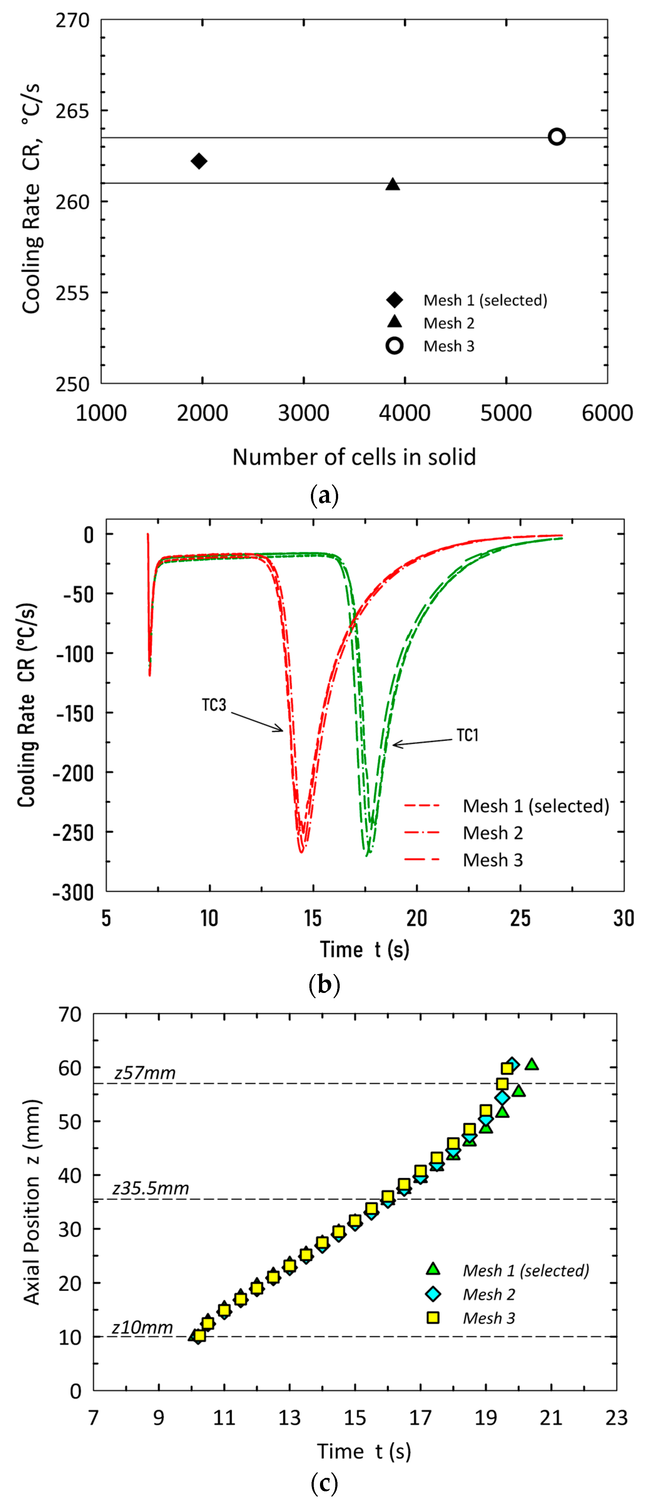
Figure 4 shows the chosen mesh, which consists of 3567 elements in the whole computational domain with an average orthogonal quality of 0.98.
Figure 5a–c shows the sensitivity mesh analysis for the solid probe in case V1.
Figure 5a shows the computed maximum cooling rate for three different numbers of cells. The results are essentially mutually equivalent, and therefore the mesh having the smaller number of elements was chosen.
Figure 5b presents the computed cooling rates for two thermocouple positions as a function of time. There is no significant difference between these results. Finally,
Figure 5c shows the computed position of the wetting front during quenching, and the results are again practically independent of the used mesh.
3.4.2. Numerical Solution
The mass, momentum, and energy conservation equations were solved using the finite volume method [
9] implemented in the 2018 ANSYS
® Fluent code. Simulations were conducted for the cases shown in
Table 3 and included 25 s of the quenching process using a time step of 0.001 s. Convergence was achieved with a residual value of 10
−3 for continuity and momentum equations, while a value of 10
−6 was applied for the energy equation.
5. Summary and Conclusions
This work presents a heat transfer and boiling model to understand and predict the thermal evolution of a solid probe under forced convection quenching. The conservation equations of mass, momentum, and energy were numerically solved together with the turbulence k-w SST (Shear Stress Transport) and thermal radiation, Discrete Ordinate (DO), differential equations, subjected to proper initial and boundary conditions. The wall heat flux was computed in all three boiling regimes using a single semi-mechanistic equation rather than specific empirical equations to represent each boiling regime. Furthermore, the model is computationally efficient since it solves the interpenetrated phase equations for the vapor-liquid water mixture, avoiding the more computationally expensive calculation of the vapor-liquid interphase for every bubble.
An original feature of this work is the validation method for this type of model. A combination of two laboratory measurements was used for validation: (1) the recorded wetting front motion along the surface of a conical-end cylindrical probe, and (2) the cooling curves obtained with four sub-superficial thermocouples in the probe. The first measurements validate the accuracy of fluid flow and boiling modeling, while the second measurements are aimed at validating heat conduction calculations within the probe.
The wetting front motion was accurately represented during its displacement along the vertical wall of the conical-end cylindrical probe. The computed wall heat flux and vapor layer profiles along the probe show the simultaneous presence of the three boiling regimes: stable vapor film, nucleate boiling, and single-phase convection. This is consistent with recorded images, which also show the regime distribution during the quenching process. Model predictions seem to be more accurate for the case with a higher water velocity. This suggests that model assumptions are better suited for full forced convection.
The predicted cooling curves at the four thermocouple positions agree reasonably well with the corresponding measured curves in all boiling regimes: stable vapor film, nucleate boiling, and single-phase convection. A more sensitive comparison between calculations and measurements is the curve of cooling rate versus time. The computed cooling rates also agree with the measured values. The computed temperatures of maximum cooling rates at the thermocouple locations match perfectly with the corresponding measured values for case V1, water velocity 0.6 m/s, and initial probe temperature 930 °C. For case V2, which has a lower water velocity, there is no such thing as a perfect match but a fair agreement. Furthermore, the computed maximum cooling rate values are consistently higher than those measured. It is not clear whether this can be attributed to experimental error or model assumptions.
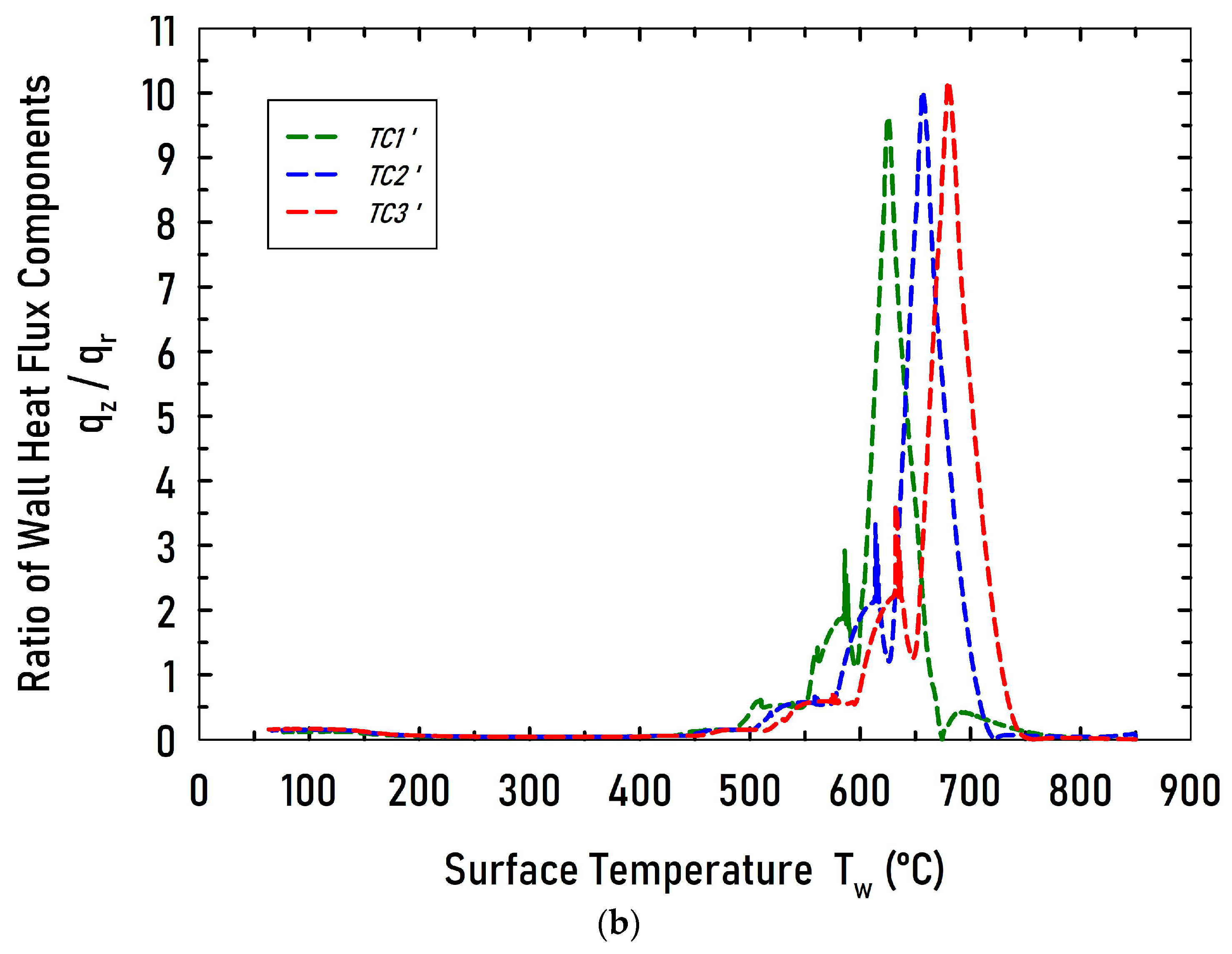
Finally, the model was used to determine the ratio of heat flux components, qz/qr, at the wall at the thermocouple z-positions. It was found that the axial component can be up to 5 times larger than the radial component for case V1, and up to 10 times larger than the radial component for case V2. This is a result of having all three boiling regimes simultaneously distributed along the wall. This multi-regime boiling phenomenon is undesirable since it leads to non-uniform wall heat flux and potentially poor workpiece quality. Finally, one-dimensional IHCP analysis is not appropriate to determine the wall heat flux when multi-regime boiling is present. Two-dimensional IHCP analysis and using thermocouples embedded along radial and axial directions should be preferred.


 ,
, 


