Article

A Thermo-Structural Analysis of Die-Sinking Electrical Discharge Machining (EDM) of a Haynes-25 Super Alloy Using Deep-Learning-Based Methodologies

by
T. Aneesh
1,†,
Chinmaya Prasad Mohanty
1,†,
Asis Kumar Tripathy
2,
Alok Singh Chauhan
3,
Manoj Gupta
4 and
A. Raja Annamalai
5,*
1
School of Mechanical Engineering, Vellore Institute of Technology, Vellore 632014, India
2
School of Computer Science Engineering and Information System, Vellore Institute of Technology, Vellore 632014, India
3
Defence Metallurgical Research Laboratory, Defence Research and Development Organisation, Hyderabad 500058, India
4
Department of Mechanical Engineering, National University of Singapore, Singapore 119077, Singapore
5
Centre for Innovative Manufacturing Research, Vellore Institute of Technology, Vellore 632014, India
*
Author to whom correspondence should be addressed.
These authors contributed equally to this work.
J. Manuf. Mater. Process. 2023, 7(6), 225; https://doi.org/10.3390/jmmp7060225
Submission received: 16 October 2023 / Revised: 4 December 2023 / Accepted: 6 December 2023 / Published: 13 December 2023
(This article belongs to the Special Issue Advances in Metal Cutting and Cutting Tools)

Abstract

:
The most effective and cutting-edge method for achieving a 0.004 mm precision on a typical material is to employ die-sinking electrical discharge machining (EDM). The material removal rate (MRR), tool wear rate (TWR), residual stresses, and crater depth were analyzed in the current study in an effort to increase the productivity and comprehension of the die-sinking EDM process. A parametric design was employed to construct a two-dimensional model, and the accuracy of the findings was verified by comparing them to prior research. Experiments were conducted utilizing the EDM machine, and the outcomes were assessed in relation to numerical simulations of the MRR and TWR. A significant temperature disparity that arises among different sections of the workpiece may result in the formation of residual strains throughout. As a consequence, a structural model was developed in order to examine the impacts of various stress responses. The primary innovations of this paper are its parametric investigation of residual stresses and its use of Haynes 25, a workpiece material that has received limited attention despite its numerous benefits and variety of applications. In order to accurately forecast the output parameters, a deep neural network model, more precisely, a multilayer perceptron (MLP) regressor, was utilized. In order to improve the precision of the outcomes and guarantee stability during convergence, the L-BFGS solver, an adaptive learning rate, and the Rectified Linear Unit (ReLU) activation function were integrated. Extensive parametric studies allowed us to determine the connection between key inputs, including the discharge current, voltage, and spark-on time, and the output parameters, namely, the MRR, TWR, and crater depth.

1. Introduction

Potential drop spark machining has emerged as a highly advanced and effective alternative technique for the removal of materials. The principal application of electrical discharge machining in the automotive, aerospace, and medical sectors [1,2,3] is the production of intricate dies, molds, and other sensitive and exacting components. Regardless of the hardness of the material or workpiece, it can be machined using this technique by utilizing thermal energy generated by an electrical discharge. In relation to the chemical underpinnings of the operational procedure, the instrument and the workpiece function as the terminal anode and cathode, respectively. Material degradation occurs more rapidly at the anode compared to the cathode; therefore, the anode suffers the consequences. By means of this program, it is possible to optimize the MRR while minimizing the TWR. Consequently, the overall productivity of the process might experience an upward trend. Furthermore, a continuous-flowing dielectric medium is employed to enhance the efficacy of the charge transfer. Machining a rigid material to near-perfect tolerance levels using conventional machining processes is exceedingly difficult; therefore, this stands as the principal advantage of the EDM process.
However, the EDM method is associated with drawbacks such as poor material evacuation and greater erosion of the electrodes. In some cases, the surface integrity and residual stress developed on the machined surface are big concerns for tool engineers [1,3,4,5]. A multitude of inquiries conducted in previous studies have endeavored to identify solutions to these challenges. However, when involving the behavior of spark discharges, it is really difficult to observe the process experimentally and quantify the responses. Therefore, it is vital to predict the responses numerically by using a simulation approach for the proper identification of EDM responses and the minimization of non-beneficial parameters, such as the greater erosion of tools and higher residual stresses.

2. Literature Review

The process of electrical discharge machining has been studied meticulously since the early 1970s. By comparing a simulator and experimental data obtained with a variety of instruments, the optimal combination of parameters for cutting was ascertained. A thermal model devised by Tiwari et al. [6] utilized M2 tool steel for the workpiece in order to was to examine the impact of the discharge current, duty factor, and discharge duration on the MRR. In their study, Patel and Powar [7] conducted a numerical comparison between the crater volume simulated by EDM on AISI 1040 steel and measurements obtained from actual EDM operations. An investigation was conducted by Kumar et al. [8] into the reliability of the spark radius in relation to the discharge current and duty cycle. In addition to conducting a finite element analysis of the powder mixed EDM process (PMEDM), Desai and Kavade [9] investigated several critical factors, including heat distribution and material ejection efficacy. In order to examine the influence of input variables, such as the discharge current and discharge voltage, on crucial output process parameters, including the tool attrition rate and material removal rate, CP Mohanty et al. [10] constructed a 2D axisymmetric model. In order to predict the dimensions of craters, an experimental investigation was conducted by Jilani ST and PC Pandey [11] regarding the depth-to-diameter ratio of craters generated via EDM, and the results revealed that the material removal process was not substantially impacted by the pulse form. Experimental research was conducted by Halkaci HS and Arden A [12] to determine the sources of surface roughness and the effect of all process parameters on the same.
The effectiveness of the EDM process in performing secondary finishing operations has also been investigated by previous researchers. The feasibility of using EDM for roughening and finishing operations was investigated by Amorim et al. [13] using AISI P20 steel and a copper electrode. In their EDM investigation of Inconel 825, A. Mohanty et al. [14] examined the surface finish and the rate of material elimination in relation to the peak current and pulse duration. In an effort to increase process efficiency, Joshi S. et al. [15] investigated the application of a pulsating magnetic field as a component of a hybrid optimization strategy. In order to investigate the effects of the discharge voltage and pulse duration on the crater depth, radius, and MRR, Dastagiri M. and Kumar AH. [16] developed a thermal simulation model. Oßwald, K. et al. [17] investigated the energy distribution in EDM experiments by utilizing the measured temperature curves. Akshay Dwivedi et al. [18] optimized the process parameters and examined the effects of the pulse current, gap control setting, and flushing pressure on the Al 6063 metal matrix composite using Taguchi’s method. An experimental study conducted by Prasad AR et al. [19] examined the material removal rate and surface roughness during the wire EDM procedure. Additionally, the analysis of variance method was utilized to optimize the process configuration. To examine the effects of various process variables on aluminum matrix composites, D. Palanisamy et al. [20] conducted an investigation. Ramakrishnan and R. Karunamoorthy [21] used DOE for multi objective optimization of EDM.A numerical investigation was conducted by Somashekar KP et al. [22] using a two-dimensional heat equation. They concluded that correlations between temperature, surface convection, and spark ratio timings in the context of multispark discharges can be calculated using the finite volume method.
From analyzing studies dealing with the application of deep-learning methods to general research studies, Yann LeCun et al. [23] reached the conclusion that research, object identification, and genomics have been significantly enhanced via deep-learning computations and models. In their work, Du-Ming Tsai and Yi-Hsiang Chou [24] introduced a deep neural network regression model that aims to enhance the precision and efficiency of image alignment. Ikai T and Hashigushi K [25] developed heat flux equations and studied the process of crater formation in detail. Wuyi Ming et al. [26] utilized optimization methods, including the adaptive-network-based fuzzy interference system (ANFIS), to achieve optimal exhaust emission characteristics and efficiency per volume. The desirability function was employed by Rafał Ŗwiercz et al. [27] to optimize surface irregularity, white layer thickness, and MRR. Kuwar Mausam et al. [28] improved the MRR and TWR by optimizing the peak current, duty factor, and gap voltage using gray relational analysis (GRA). Therefore, it is indisputable that the methods of deep learning have been extraordinarily beneficial and efficient in attaining a more comprehensive and precise understanding of the subject under investigation. C.P Mohanty et al. [29] optimized the machining process of EDM using a particle swarm approach.
Regarding the implementation of EDM in machining unconventional materials, Jain A et al. [30] reviewed the feasibility of using several machining processes in the secondary activities of fiber refinement polymer composites (FRPCs) and concluded that unconventional methods are both convenient and well established. R. Kirubagharan et al. [31] studied the effect of electrode sizes on parameters such as the MRR and surface roughness of Inconel X750, along with the implementation of a Taguchi design for experimental work. W. Ming et al. [32] reviewed the advantages of EDM in machining advanced ceramics when compared to traditional machining methods, along with using workpiece electrical conductivity and surface topography to increase the process efficiency. S. Boopathi [33] conducted a review on the near-dry EDM process, which is an upcoming technique in which the liquid dielectric fluid is replaced with a gas or gas mist in order to make the overall process more ecofriendly. Grigoriev S.N. et al. [34] conducted an extensive study on the process of EDM of a ceramic nanocomposite using water as well as mineral oil with discharge factors, wire tool behavior, tool material evaluation, and medium influence. Papazoglou EL et al. [35] conducted an experimental study on the machining of titanium grade 2 with EDM using the MRR, TWR, and average white layer thickness as performance indexes. V. Prakash et al. [36] studied the usability of EDM and micro-EDM on unconventional hard-to-machine materials, such as nickel alloys, titanium alloys, stainless steel, and advanced ceramics. Abu Qudeiri J.E. et al. [37] reviewed the capability of EDM in machining different grades of stainless steel along with various attempts made at process improvement by optimizing the MRR and surface quality. R. Chaudhari et al. [38] investigated the effectiveness of wire EDM in preserving the surface integrity during the machining of nitinol shape memory alloy (SMA) through various microscopy imaging techniques. R. Singh et al. [39] conducted an extensive literature study and reported that the proper selection of the process variables, tool electrode, and dielectric can play an important role in improving EDM process efficiency. Bui V.D et al. [40] studied the feasibility of EDM in manufacturing medical grade equipment. Pramanik. A et al. [41] optimized the aspect of dimensional accuracy in wire EDM.

Identified Research Gaps

From the exhaustive literature study, it is evident that a substantial amount of effort has been devoted to the study and investigation of this subject. However, it is also evident that the majority of previous research has been conducted on workpieces made of common materials such as steel alloys and aluminum [1,2,3,4,7,13,14,37]. Aeronautical materials, which are among the most critical applications of the EDM process, have received almost no research attention. Based on the literature review presented above, it is apparent that there is a scarcity of research examining the residual stresses that develop in the workpiece throughout the machining process, as well as the various parameters that may influence their extent [3,8,10]. Furthermore, it is worth noting that the implementation of deep-learning methods, such as neural networks and other novel multi-response optimization techniques, to predict response parameters with greater accuracy, efficiency, and computation speed is limited to a small number of papers [21,23,26].
An inherent benefit of the EDM process is its capability to machine difficult materials that cannot be machined with other methods currently in use. Consequently, an important contribution of this study is its examination of the feasibility and efficacy of die-sinking EDM in the machining of Haynes 25, an unconventionally tough material. Relatively few researchers have conducted parametric studies [2,3,10], wherein the influence of each input process parameter is meticulously monitored. This type of research is essential because it provides a comprehensive understanding of the effects of a single input parameter. The majority of research has been carried out in overly idealized conditions, including a constant heat flux and a fixed flame radius [25]. Any reliance on this premise could potentially compromise the accuracy of the simulation outcomes. In determining the practical heat capacitance of the tool specimens and the workpiece, the latent heat of melting was not introduced. The majority of the material was eliminated during the machining process via a phase transition from solid to liquid, as opposed to from solid to gas. While it is possible for multiple discharges to transpire during the machining process, the majority of them transpire in close proximity to one another, with minimal distance between electrodes. Consequently, it is possible to consider them all as a singular spark. The present research study was conducted to simulate a single spark; the findings derived from this study were subsequently extrapolated to multispark operations. Comparable findings have also been reported by prior scholars [1,4].
Drawing from the aforementioned observations, it is apparent that experimental investigations utilizing sophisticated deep-learning regression methods to assess the EDM process parameters for an unprecedented Haynes-25 superalloy have been scarce. Regression models are highly advantageous when it comes to forecasting multiple outputs from a variety of inputs. Utilizing a deep-learning model, this research endeavored to create an intelligent system capable of forecasting output parameters, thus substantially augmenting the efficiency of machining operations. In this study, critical parameters such as the material removal rate (MRR), tool wear rate (TWR), and crater depth were analyzed in relation to process variables, including the discharge current, voltage, and spark-on time. To achieve this, an advanced deep-learning approach was utilized, specifically a deep neural network, namely, the MLP regressor. In addition, kernel density estimates (KDEs) were produced in order to graphically depict the density of data points across a range of values, with a specific focus on the MRR, TWR, and crater depth.

3. Methodology and Technical Specifications

3.1. Procedure Overview

First, a 2D axisymmetric model was developed, and then the workpiece material’s temperature-dependent properties were included in it. After that, the requisite values were computed and incorporated into the model, in conjunction with the initial conditions, boundary conditions, and varying heat flux values. Following that, a temperature distribution contour that was deemed valid was acquired through the implementation of all requisite solution and analysis controls in the simulation segment. Subsequently, the node numbers of the elements whose temperature readings were significantly greater than the Haynes 25 melting point temperature were determined. Subsequently, the material removal rate (MRR) was computed by employing the EKILL function of Ansys APDL to eliminate elements whose temperature readings exceeded the melting point of Haynes 25 material. The measured dimensions of the formed crater were incorporated into the MRR calculations accordingly. The method outlined earlier was replicated in order to compute the tool wear rate (TWR), albeit with distinct boundary conditions and copper material properties. Following the determination of the MRR and TWR, a structural model incorporating diverse element types was constructed to compute the residual stresses that may arise in the workpiece. This was accomplished by implementing appropriate displacement constraints and utilizing the temperature distribution acquired from prior thermal simulations. Following the conclusion of all simulations, experiments were carried out utilizing a Haynes 25 workpiece and copper electrode to compute the MRR and TWR through the implementation of the weight reduction experimental technique. Subsequently, the established simulation model was verified through a comparison between the numerical outcomes and the experimental data. In order to determine the impact of the input variables, including the discharge current, voltage, and spark discharge duration, on output process parameters, including the MRR, TWR, residual stresses, and crater depth, a comprehensive parametric study was conducted.

3.2. Experimental Methodology

The investigations were conducted using the EDM machine model PSR 35 C425, which is accessible from the Vellore Institute of Technology (VIT), Vellore. The discharge current was adjusted within the range of 10 A to 20 A, whereas the spark-on and spark-off times were varied between 100 and 300 μs and 28 and 48 μs, respectively. In addition, the discharge voltage was varied between 30 V and 50 V across all experimental combinations. A comprehensive analysis was conducted on every conceivable combination resulting from these variations. The resulting data were then extensively examined in order to ascertain the impact that each input parameter had on the final response parameters. As a dielectric, a particular hydrocarbon oil was utilized in the experimental procedure.

3.3. Workpiece Material Properties

The Haynes 25 alloy is an unorthodox material composed primarily of cobalt and a number of additional alloying elements. Strong resistance to corrosion caused by both hot and chemical oxidations, high-temperature properties, and excellent formability are among its most notable attributes. Owing to these characteristics, it finds predominant application in the fabrication of high-temperature furnaces, turbine rings, combustion chambers, and afterburner components. Table 1 and Table 2 detail the physical and temperature-dependent characteristics of the Haynes 25 alloy.

3.4. Tool Material Properties

Copper (Cu) is a highly ductile, flexible, and malleable substance with tremendous thermal and electrical conductivity [5]. Copper is utilized in a multitude of electrical and structural applications, including the fabrication of electrodes, electric motors, wires, cables, and more; in situations where a high surface finish is required, the EDM process is enhanced by employing copper electrodes. Using a copper electrode as the instrument has one disadvantage, which is the increased complexity and simplicity of detail. The properties of the copper instrument are detailed in Table 3.

3.5. Governing Equations

In order to simulate the EDM process, the Fourier heat conduction equation is utilized, as illustrated in Equation (1). In this equation, the following variables are considered: the temperature (T), specific heat capacity (Cp), density (ρ), and thermal conductivity (Kt) of the workpiece material. Analogous analyses have been documented in prior scientific investigations [2,3].
1 r r K t r T r + z K t T z = ρ C p T t
Regarding the boundary conditions, it is initially postulated that a uniform temperature of 300 K exists throughout the elements of the workpiece while it is submerged in the dielectric. A portion of the workpiece surface (Rpc) that is approximately one-tenth of the model dimensions is subjected to a varying equational heat flux [3]. In contrast, the remaining boundaries are governed by a conventional boundary condition, as illustrated in Figure 1. All remaining surfaces of the workpiece are insulated, and corresponding boundary conditions are established for these surfaces as well.
The heat input plays a critical role in determining the material removal rate and cavity dimensions during the machining process. Nevertheless, numerous prior investigations have been conducted with the supposition of a uniform heat flux. The derived simulation results are compromised in terms of accuracy and precision due to the oversimplification of these assumptions. Diverse methodologies have been employed by numerous researchers in the development of spark radius equations. Ikai and Hashiguchi [25] have formulated a semi-empirical equation for the spark radius that is well regarded by numerous prior researchers [1,2,3,6,10] on account of its high degree of predictive accuracy among the existing literature. Therefore, as stated in Equation (2), the spark radius at the work surface (Rpc) is considered to be a function of the discharge current (I) and pulse-on time (Ton) in this study.
R p c = ( 2.04 × 10 3 ) × I 0.43 × T o n 0.44
Equation (3) represents the assumption that the heat emitted by the EDM discharge into the workpiece follows a Gaussian distribution [1].
q w r = 4.45 × P × V × I π × R p c 2   e x p { 4.5 r R p c 2 }
Therefore, through additional simplification and the substitution of Equation (2) for Equation (3), the final heat flux equation (qw(t)) is derived, as specified in Equation (4). This equation shall be utilized in subsequent analyses for the remainder of the present manuscript.
q w t = 3.4878 × 10 5 F c V I 0.14 T o n 0.88   e x p 4.5 t T o n 0.88
where F C is the fraction of total power going to the cathode, V is the discharge voltage, and I is the discharge current.

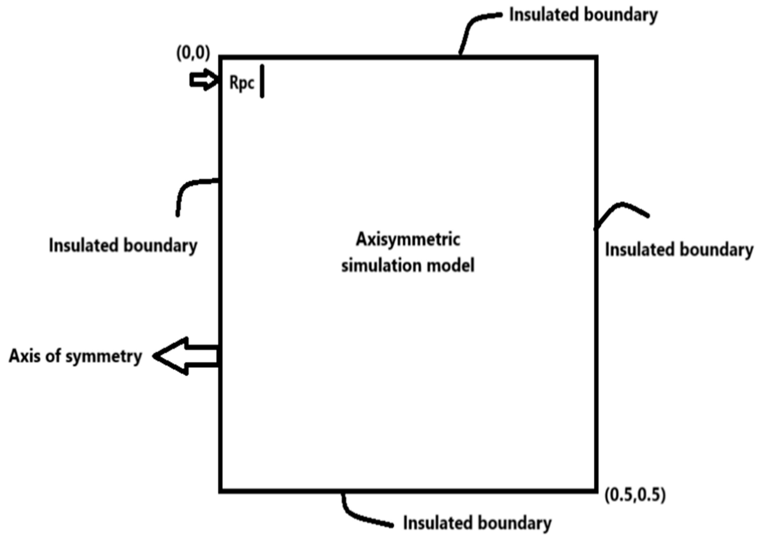
3.6. Design Approach Details

As illustrated in Figure 2, a 2D axisymmetric square model measuring 0.5 × 0.5 mm was constructed utilizing the ANSYS APDL 2022 R1 software in order to conduct the FEA simulation. The simulation utilized these specific dimensions due to the requirement that the model dimensions be ten times the spark radius obtained [3]. A 5 μm lattice was implemented across the entire workpiece utilizing a mesh tool. By optimizing the region encompassing the heat flux, we were able to enhance the precision of the acquired outcomes while minimizing the computational burden. Four thermal solid elements per node were incorporated into the model’s design (PLANE 55). The foundation of the object is illustrated in Figure 2.

3.7. Assumptions in the Proposed Model

The following are the assumptions taken into account in the present study:
  • Both the tool and substrate materials demonstrate isotropy and homogeneity in their microstructures.
  • The predominant mode of heat transfer from the plasma to the electrodes during the EDM process is conduction. Simultaneously, radiation and convection contribute significantly to the heat transfer from the plasma to the dielectric. In the present inquiry, it is postulated that conduction serves as the predominant means of heat transfer from the plasma to the electrodes.
  • It is assumed that the radius of the spark produced during EDM is a function of the spark duration and discharge current.
  • A Gaussian distribution is applied to the heat flux, and it is supposed that the area where the spark is applied possesses axisymmetric properties.
  • The workpiece is effectively exposed to only a small portion of the applied spark energy, with the remainder being lost due to dielectric convection and radiation.
It is presumed that the flushing efficiency of the dielectric is one hundred percent and that there is no recast deposition on the surface of the workpiece.

4. Results and Discussion

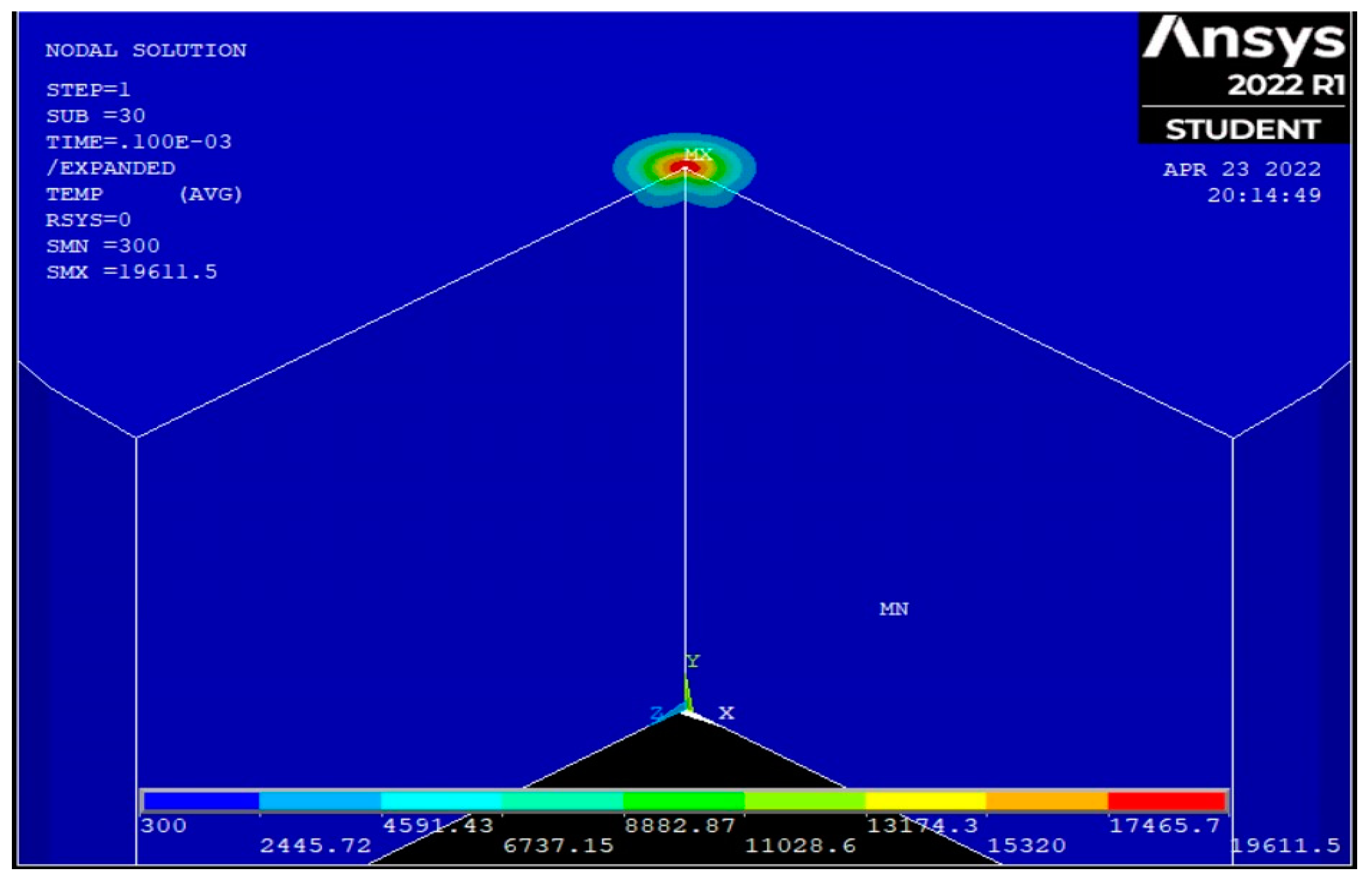
4.1. Simulation Results

The initial development of a two-dimensional continuous figure measuring 0.5 × 0.5 mm was performed utilizing the ANSYS Parametric Design Language. The necessary boundary conditions and the governing heat flux equation were implemented. Following the application of the properties that are dependent on temperature, the temperature distribution for a specific set of input parameters was computed. Figure 3 illustrates a sectional view of the temperature distribution subsequent to the application of a spark with a heat flux of 100 μs, a current of 10 A, a spark-on time of 100 μs, and a discharge voltage of 40 V. Following this computation, the APDL-implemented EKILL technique was utilized to identify and eliminate from the workpiece any nodes with a temperature reading exceeding its melting point. As a consequence, a bowl-shaped crater developed in the vicinity of the discharge source. Figure 4 illustrates the crater composed of input parameters that are comparable to those described above. The dimensions of the resulting crater are 40 μm in depth and 56 μm in radius.
A simulation model resembling the aforementioned model was developed, incorporating temperature-dependent material properties obtained from reference [5] and the boundary conditions illustrated in Figure 1. This model was utilized in the FEM analysis to calculate the tool attrition rate of the copper tool. Figure 5 and Figure 6 depict the temperature distribution and crater cavity that result from the elimination of elements whose melting point temperature is greater than that of the tool specimen, respectively. The cavity that was generated possessed a crater depth of 16 μm and a radius of 25 μm.

4.2. Residual Stresses Occurring in the Workpiece

Due to the formation of a significantly elevated temperature gradient within the workpiece, stresses will accumulate, potentially leading to surface integrity degradation and the prolonged operational lifespan of the machined body. In order to generate residual stresses via simulation, APDL was utilized to construct a two-dimensional structural model, which was subsequently modified with PLANE 182 to facilitate the structural analysis. Following the application of structural properties such as Poisson’s ratio and the modulus of elasticity, the requisite boundary conditions were established by imposing displacement constraints. By transferring the temperature distributions from prior thermal simulations to the present structural environment, the residual stresses were subsequently estimated. Figure 7 illustrates the resolution of Von Mises stresses that arise in the workpiece subsequent to the removal of material. Based on the findings, it can be deduced that the machining process will induce a composite of compressive (negative) and tensile (positive) stresses in the workpiece, as shown in the figure. The considerable magnitudes of these stressors have the potential to induce a multitude of structural integrity issues, including but not limited to diminished fatigue life, dimensional instability, distortion, warping, stress corrosion cracking, compromised machinability, and machining strength.

4.3. Experimentation

A total of 29 experimental trials were performed with an average machining time of 340 s in order to ascertain the impact that different levels of input parameters would have on the levels of the response parameters. Before initiating the EDM process, thorough cleansing was conducted for both specimens in order to eliminate any superfluous inclusions. The specimens employed as the materials for the workpiece and tools, respectively, are copper and Haynes 25. These materials are visually represented in Figure 8. Following each experiment, a comparison was made between the weights of the two experimental specimens to ascertain the amount of material that was removed during each phase of the investigation. After obtaining all the required values, the experimental material removal rate and tool attrition rate were calculated using Equation (5), in which ρ represents the density of the workpiece and tm signifies the duration of the machining process.
M a t e r i a l   r e m o v a l   r a t e = I n i t i a l   w e i g h t f i n a l   w e i g h t ρ × t m

4.4. Model Validation with Experimentation

An assumption underlying the simulation model presented in the present study is that a single discharge occurs. However, in practice, the EDM process is governed by a multitude of factors that affect its dynamics. These include a minor delay in ignition, flushing efficiencies below 100%, irregular melting of the electrode and workpiece, impurities in the dielectric oil, and the randomized motion of machined particles during the machining procedure. It is nearly impossible to incorporate all of these variables into simulation process models. Therefore, the simulation was conducted under process conditions where each spark exhibited exceptional and uniform efficiency. Following the completion of the experimentation, as described in the preceding sections, simulations were executed utilizing input parameters that mirrored the experimental inputs. The subsequent experimental results as well as the simulation results, illustrate the effects of 5% energy reaching the workpiece and 6% energy reaching the tool. In order to determine the experimental residual stresses, the X-ray diffraction technique was implemented (Bruker D8 Advance). The purpose of precisely homogenizing the material in this XRD method is to ascertain its bulk composition. By suspending the material in the air and permitting a monochromatic beam to traverse it, an examination of all possible reflections is conducted. This analysis provides valuable information regarding the crystalline aberrations that developed as a consequence of residual stresses and their magnitudes.
Through a comparison of the experimental and simulation results presented in Table 4, it is possible to discern that the error percentage falls below the acceptable threshold, and the two sets of results exhibit a high degree of concordance. After this, another set of experiments was carried out in similar conditions but with a shorter machining time of 5 s, and the results are shown in Table 5. The aim behind the application of a shorter machining time was to reduce the number of discharges on the workpiece as much as possible for better accuracy while comparing the crater dimensions [3]. Table 5 compares the crater depths obtained during experimental and simulation runs conducted under identical conditions in an effort to establish a stronger correlation between the two sets of results. Figure 9 shows the comparison between the predicted crater bowl cavity and the experimental results of run no. 19 whereas Figure 10 depicts the actual image of a crater formed during the procedure.
The crater depth and crater radius, shown in Table 5, were measured using a Mitutoyo TM 500 measuring microscope that has a dimensional accuracy of 0.005 mm and can reach an effective magnification of 30× using the combination of the eyepiece and objective lens. Initially, the workpiece was mounted onto the stage glass using a holder with a clamp. After selecting an appropriate mode of illumination and positioning, the crater diameter was measured using a micrometer head, through which the radius was further calculated. In order to measure the crater depth, a combination of a Z-axis micrometer head, height measurement attachment, and a dial indicator was used. The microscope was initially calibrated using a standard material with known dimensions, and the measurements were repeated multiple times to ensure accuracy and account for variations.

4.5. Model Validation with Prior Reputed Research Works

In order to ascertain the reliability and precision of the current simulation model, a simulation study was conducted utilizing input parameter levels comparable to those utilized by Joshi and Pande [3]. In addition to the other parameter levels taken into account in the current analysis, the machining conditions were identical to those of their simulation model. The MRRs of the anticipated outputs from both simulation models are illustrated in Table 6. In a similar fashion, an evaluation of the TWR was conducted. Figure 11 illustrates a graphical comparison of the MRR and TWR outcomes of our model with those of the model proposed by Joshi and Pande [3]. The copper instrument and the steel workpiece are two of the most important model parameters; the discharge voltage is 25 volts. Through observation and a comparison of the outcomes produced by the two models, it is possible to deduce that they are substantially congruent, thereby providing validation for our present simulation model.

5. Parametric Studies on the Proposed Thermo-Structural Model

A multitude of parametric investigations were carried out across a wide range of input parameter levels utilizing the validated simulation model. The principal objective of the present investigation is to ascertain the correlation between the discharge voltage, current, and discharge current as input parameters and the resulting characteristics, including the crater depth, radius, and MRR. Table 1 presents the material properties of the Haynes 25 alloy. The input parameters listed below were obtained from the machining manual and reference [10]:
  • Discharge current: 5 A, 15 A, 25 A, 35 A, 45 A;
  • Spark on time (ton): 50 μs, 100 μs, 300 μs, 500 μs, 700 μs;
  • Discharge voltage: 20 V, 30 V, 40 V, 50 V, 60 V;
  • Duty factor: 65%, 80%, 95%.

5.1. Effect of Discharge Current

In the EDM process, the discharge current is a critical input parameter that must be taken into account due to its correlation with the energy of the sparks that are produced. Figure 12 illustrates that the MRR increases linearly with the discharge current at various discharge voltage levels. The trends identified in this parametric study correspond well to those documented by prior researchers [2,6,10]. As a result, it is advisable to utilize higher discharge current levels when performing heavy-duty machining, while post-processing and finishing operations require lower current levels. The correlation between the current and crater depth is illustrated in Figure 13. It increases monotonically at lower discharge current levels, and after a certain extent, the depth increases dramatically. Lower discharge current levels are therefore advised in order to achieve a more consistent and seamless surface finish. It is apparent from Figure 14 that the initial stages of the current increase result in a marginal rise in the TWR. However, as the discharge level escalates, a significant increase in the TWR becomes apparent, leading to a reduction in both process efficiency and cost-effectiveness [13]. As the discharge current increases, the variation in residual stresses increases dramatically, as illustrated in Figure 15. The elevated stresses will result in the deterioration of the surface integrity and fatigue life of the workpiece [10]. Therefore, selecting the optimal level of the discharge current is critical.

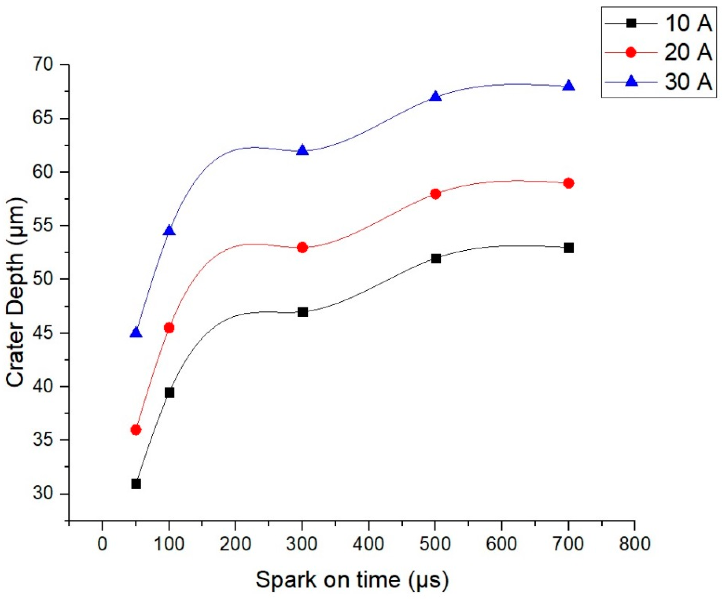
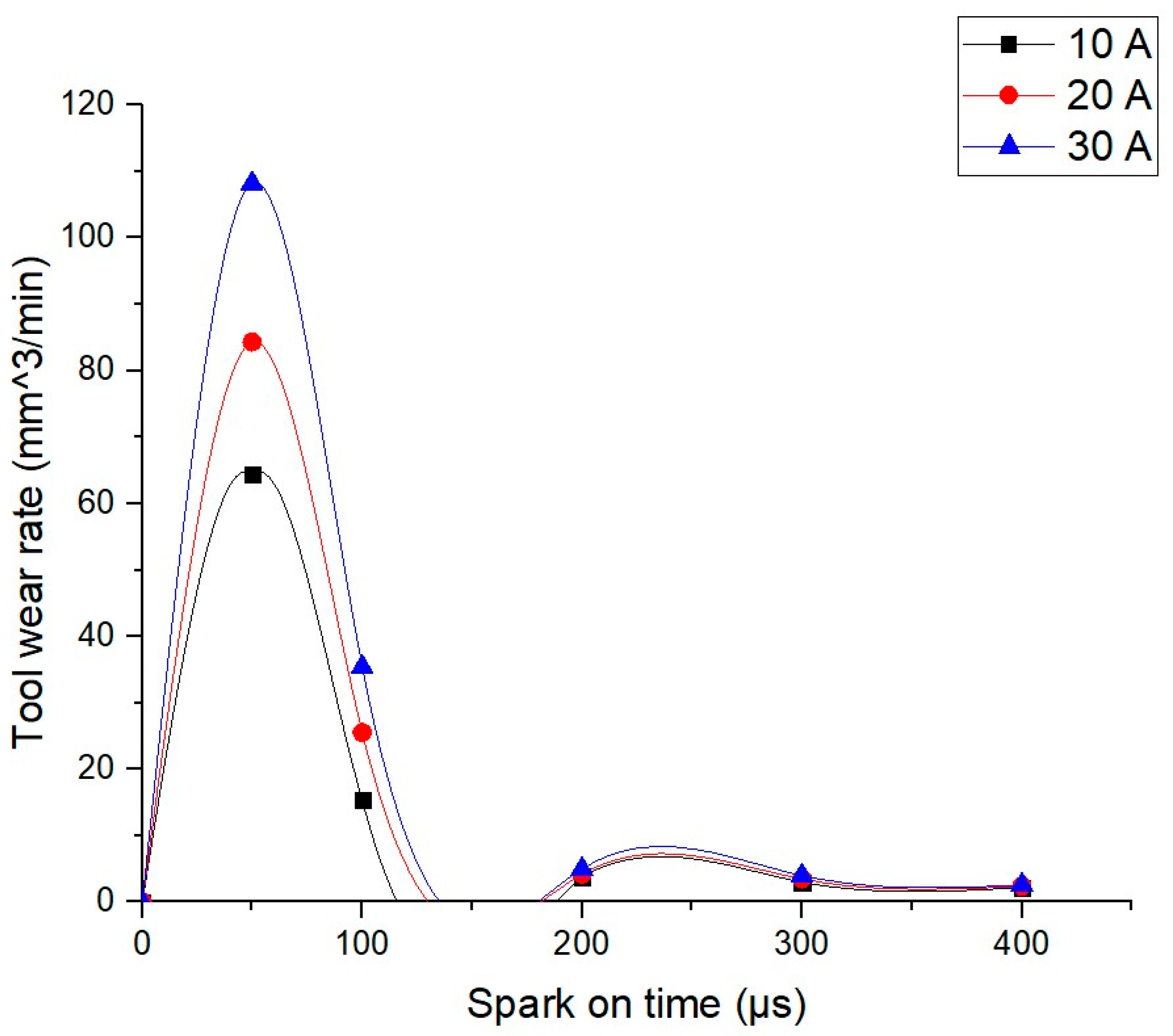
5.2. Effect of Spark-on Time

The spark-on-time effect on the MRR at different discharge current levels is illustrated in Figure 16. An initial maximum is observed in the MRR, followed by a subsequent decrease as the duration of the discharge is prolonged. This is the result of the duty factor remaining constant while the flux density decreases. This initial MRR peak has been documented in prior experimental investigations as well [4]. It increases with the passage of time, as depicted in Figure 17, but ultimately reaches a constant value. An additional observation that can be made pertains to the correlation between the discharge duration and crater cavity expansion and depth; however, this relationship is accompanied by a reduction in the material removal rate. Consequently, each spark discharge eliminates a greater quantity of material. An abrupt surge in the TWR is evident during the initial time periods, followed by a gradual decline as the spark time increases. This trend occurs due to the fact that maintaining a constant duty factor throughout the experimentation process leads to a reduction in the overall flux density and, consequently, a decline in the TWR. A decrease in residual stresses is evident as the duration of the discharge is extended, as illustrated in Figure 18. This is the case because maintaining a constant duty factor throughout the investigation causes a gradual decrease in the flux density as the study progresses, ultimately culminating in a reduction in residual stresses. Prior studies have also documented comparable patterns [10] to those illustrated in Figure 17, Figure 18 and Figure 19.

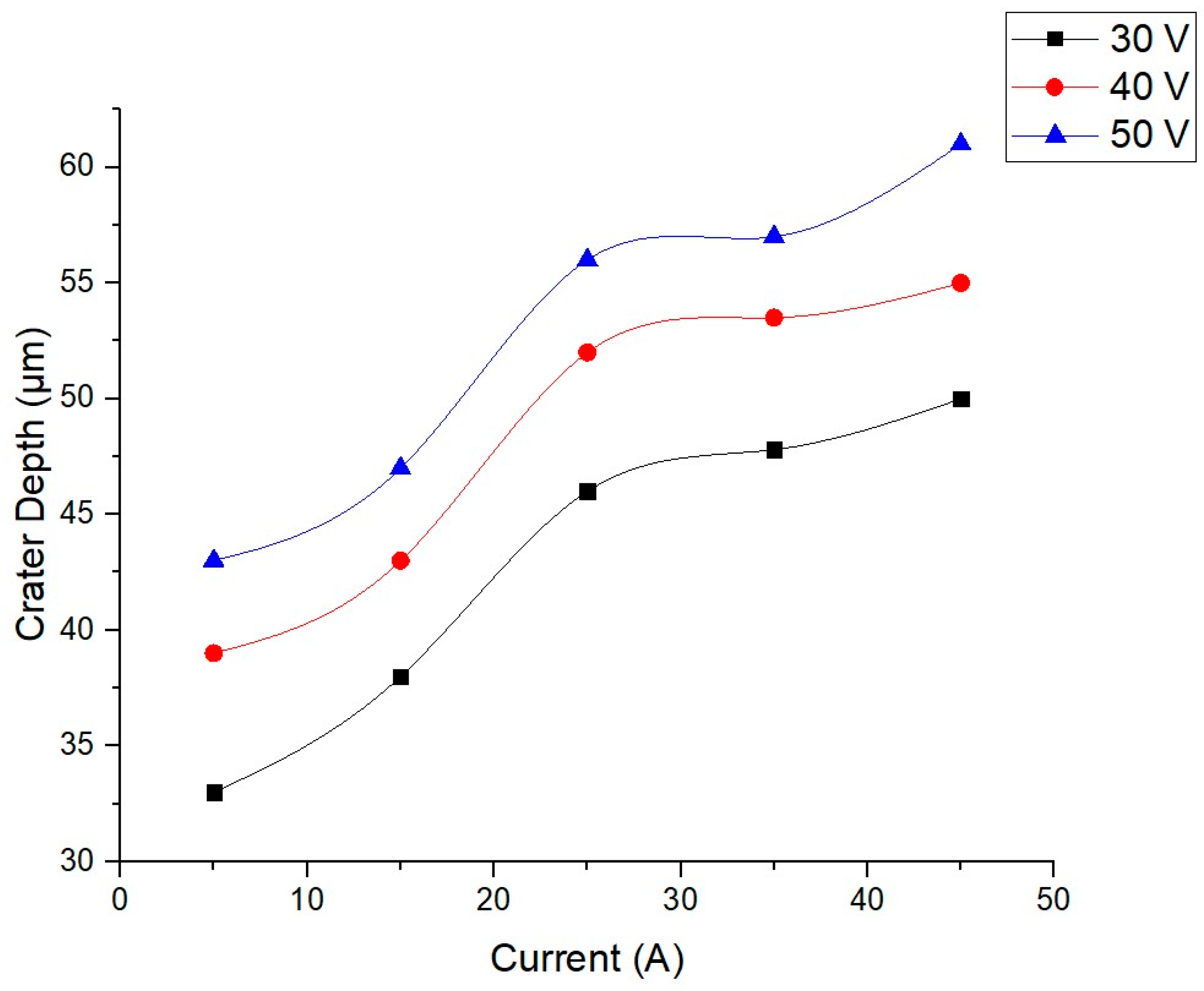
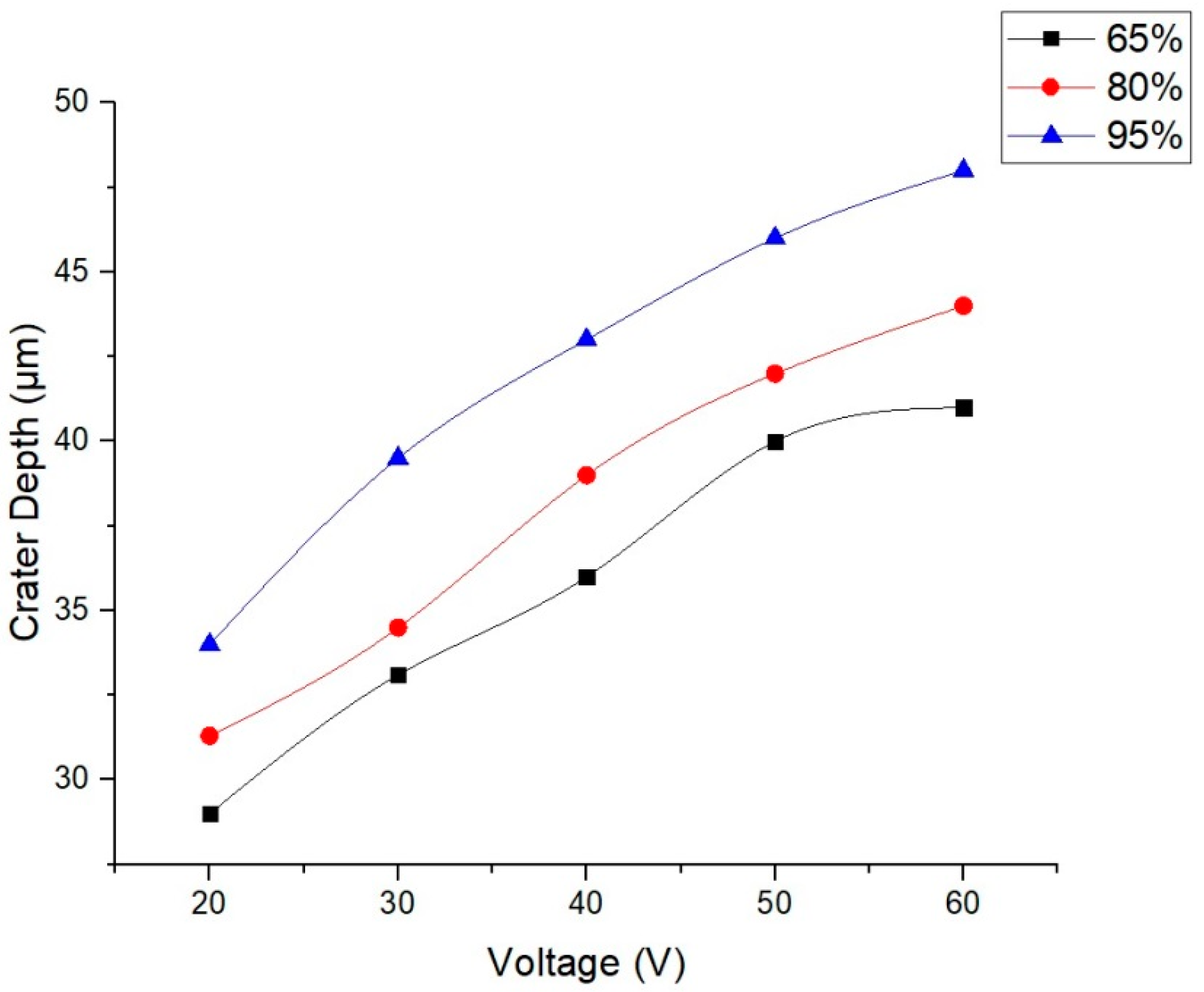
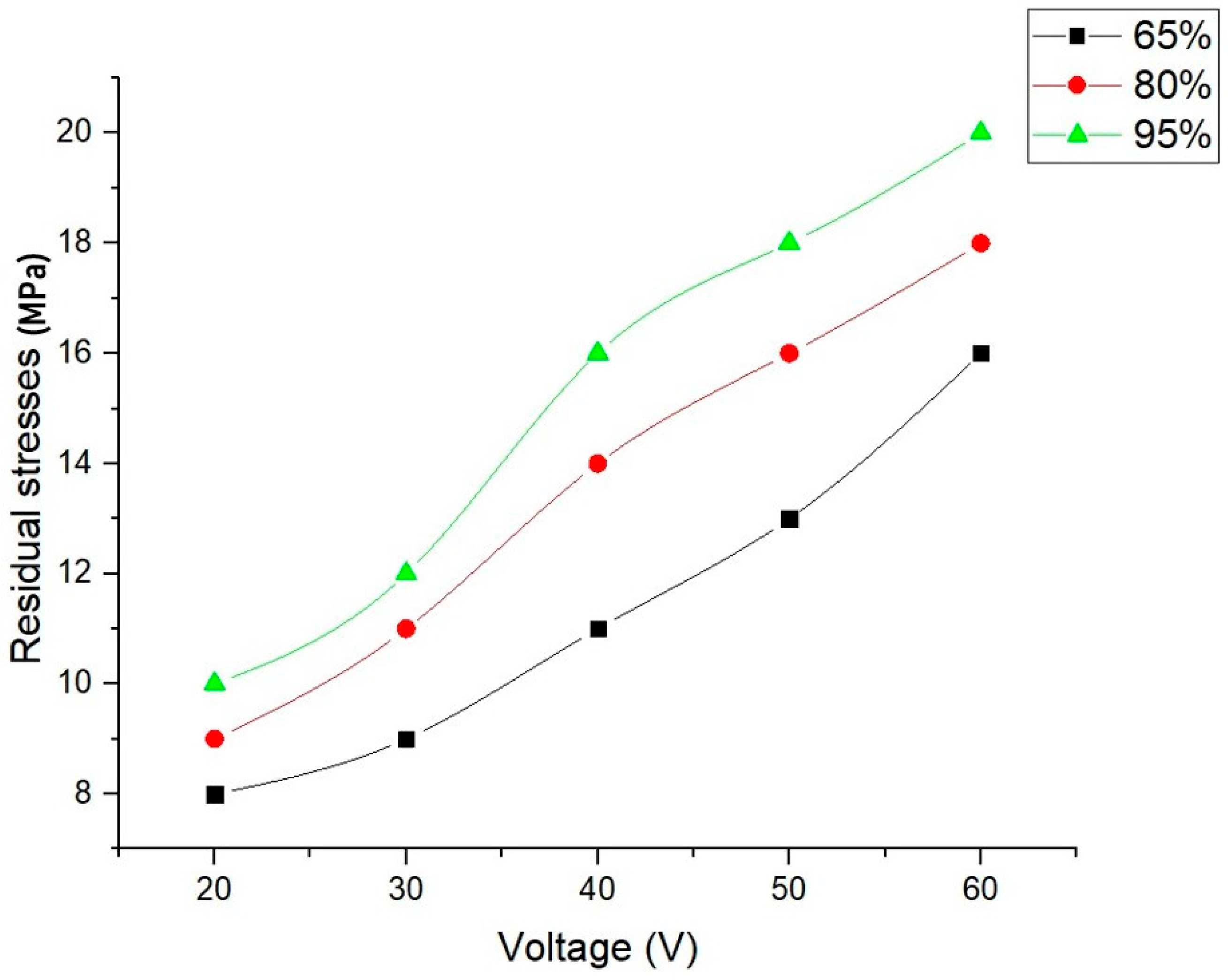
5.3. Effect of Discharge Voltage

Figure 20 illustrates the correlations that exist between the discharge voltage and material removal rate across various levels of the duty factor. The MRR increases in a linear fashion across the entire voltage range. This could be the result of increased flux density resulting from elevated voltage levels. The crater depth exhibits a comparable pattern, characterized by a marginally irregular ascent, as illustrated in Figure 21 and Figure 22, respectively. Significant residual stresses are generated with an increase in voltage, as illustrated in Figure 23. These stresses have the potential to detrimentally impact the structural integrity of the workpiece. Therefore, it can be deduced that roughening operations on workpieces are amenable to higher discharge voltage levels [3].
Based on the results of the aforementioned parametric studies, it can be deduced that the aforementioned parameters are significant factors that influence the quality of the end product and enhance the efficiency of the process. Achieving an optimal equilibrium among these four parameter levels significantly enhances the overall efficacy of the EDM process.

6. Prediction of EDM Simulation Responses Using Deep Neural Network

By employing deep-learning methodologies [23], this article forecasts a range of output characteristics, such as residual stresses, the MRR, and the TWR. The input characteristics, including the current, voltage, pulse duration, and duty factor, inform these forecasts. The developed deep-learning models are capable of comprehending the intricacies of the input features and can then predict the intended outcomes. Although the initial training phase for these deep-learning models may require a significant amount of computational time, they have the potential to generate output features with exceptional efficiency once the regression model has been successfully trained. As a result, the practicality and efficiency of applying the trained regression model to real-time manufacturing scenarios are significantly enhanced. The deep-learning approach is founded upon end-to-end neural network frameworks. In contrast to conventional approaches, it does not rely on the manual training of distinguishing features by domain experts. In contrast, it acquires knowledge from a significant quantity of annotated data samples in order to effectively train the model. Out of the variety of deep-learning models available, the neural network (NN) is identified as the most suitable architecture to tackle our issue. The neural network architecture utilized to address the regression problem is illustrated in Figure 24.

6.1. Model Selection and Training

A category of regressors known as multilayer perceptrons (MLPs) is fundamental to feedforward artificial neural networks [24]. By virtue of its input, concealed, and output layers, the architecture guarantees absolute interconnectivity among nodes spanning multiple layers. The MLP achieves nonlinear discrimination through the implementation of backpropagation in supervised learning. This is made possible through the utilization of multiple layers and nonlinear activation functions.
In this context, the MLP regressor is being employed to effectively forecast the output features pertaining to the provided problem. It is constructed from interconnected layers of neurons and undergoes training in order to forecast continuous numeric values. ‘RELU’ is the abbreviation for the Rectified Linear Unit activation function. It is frequently implemented in neural networks to accelerate training and mitigate the disappearing gradient problem. The value is returned by the “RELU” activation function if the input is positive; otherwise, it is set to zero. The phrase “adaptive learning rate” generally denotes methods in which the learning rate, which governs the size of the steps in gradient descent optimization, is modified throughout the training process in order to enhance convergence and stability. Utilizing adaptive optimization algorithms, such as RMSprop or Adam, which modify the learning rate automatically in response to previous gradients, is a common method. Particularly in neural networks, the L-BFGS (Limited-memory Broyden–Fletcher–Goldfarb–Shanno) solver is a prevalent optimization algorithm utilized in the training of machine learning models. The L-BFGS solver is employed in the context of an MLP regressor to optimize the neural network’s weights and biases throughout the training procedure. By incorporating the L-BFGS solver into an MLP regressor, we utilize this optimization algorithm to adjust the weights and biases of the neural network, with the objective of minimizing the loss function. Here, an MLP regressor model is constructed in which the neurons are activated using the “RELU” function. For more effective training, it employs an adaptive learning rate optimization algorithm and an L-BFGS solver. A total of 80% of the computed simulation results were designated for training objectives, while the remaining 20% were intended for testing.

6.2. Results and Comparisons

The variables or attributes utilized as inputs in a DL model to generate predictions are referred to as input features. The model employs these data elements as inputs in order to discover patterns and establish connections within the given data. Conversely, output metrics represent the criteria by which the effectiveness of a machine-learning or deep-learning model is assessed. As inputs, the current, voltage, duty factor, and pulse-on time are utilized, while as outputs, the MRR, TWR, and residual stresses are considered. A comparison between the features input and the features output is illustrated in Figure 25 for the purpose of evaluating the ML/DL model’s applicability. The figure is utilized to conduct a comprehensive analysis of the experimental data in order to determine the effect of each input feature on the output metrics. It is noted that none of the values, when evaluated against the input features, produce a linear output. The variation in all three output metrics is substantial, contingent upon the four input features. In the figure, the impacts of the input features “current”, “voltage”, “pulse on time”, and “duty factor” on the output metrics are analyzed in the first, second, third, and fourth rows, respectively. We decided to apply the MLP regressor, a deep-learning model, to this issue based on this observation. These metrics quantify how well the model’s predictions match the actual outcomes. Here, the output metric mean squared error is used to verify the outcome of the problem. In essence, input features are the data provided to the model, while output metrics are the measures used to assess how well the model performs based on its predictions. During the model computations, it was observed in the analysis that the linear model is not suitable for this particular problem statement. Therefore, the MLP regressor model was employed in the aforementioned investigation.
In the realm of deep learning, the term “density plot” frequently denotes a visual depiction that illustrates the estimated probability density function of a continuous variable. It can provide insight into the concentration and distribution of data elements in particular regions. Density diagrams can be utilized to visualize various aspects of data and model outputs in deep learning. Kernel density estimates (KDEs) are produced in order to visually represent the density of data points across the entire range of variables. The kernel function is commonly represented by a Gaussian distribution, and the degree of dispersion observed in the kernel graph is a crucial factor in assessing the estimation’s regularity. The KDEs of the response parameters, namely, the MRR, TWR, and residual stresses, are depicted in Figure 26.
Table 7 displays the results, along with the results of validation through confirmative tests. The simulation results are used to train a deep neural network model, which then predicts future results based on the simulation results. Based on the ideal parameter settings, which are a current value of 10 A, voltage value of 50 V, pulse-on-time value of 200 s, and duty factor value of 90%, the MRR, TWR, and residual stress values are anticipated to be 95.54, 0.24, and 9.12, respectively. It is clear from this that the predicted values are very close to the actual ones in most cases.
Figure 27 displays the expected values with the actual values. Based on the actual and anticipated values, our deep-learning algorithm picks the three best sample values to use in this graph. To find the anticipated values, the model iterates 10,000 times. The model’s anticipated MRR is higher than the observed value, but the expected TWR and residual stresses are either the same as or lower than the observed values. Furthermore, the regressor uses a regression approach to try to determine which input qualities best predict which output values. The output layer becomes linearly dependent on the input layer if we use an identity activation function there and nonlinear Rectified Linear Unit (ReLU) activation functions in the hidden layers.

7. Conclusions

A two-dimensional axisymmetric model was developed to simulate the die-sinking EDM process using ANSYS software on a Haynes 25 workpiece. The proposed model was validated through experimental approaches. Parametric studies were conducted on the proposed model to analyze the effects of vital EDM process parameters on responses. The ideal machining parameters were identified using a deep-learning-based MLP regressor equipped with “ReLU” activation and an “adaptive” learning rate, followed by validation through confirmative tests. The proposed work is useful in enhancing the EDM performance by enhancing the material evacuation ability and reducing the erosion of the tool, as well as residual stress developed on the workpiece during machining. The current in-depth analysis found the following primary findings:
  • The discrepancy between the experimental and simulation results was reduced by expressing the spark radius as a function and adding features like latent heat and Gaussian heat flow distribution.
  • Due to the large disparity in cooling rates, the workpiece experiences both tensile and compressive residual stresses during machining.
  • Haynes 25 alloy workpieces should have an energy distribution factor of 5% when calculating the final heat flux in the numerical calculations to obtain the best results.
  • As the discharge time increased, the MRR started falling after a certain period due to the decline in the flux density, although the crater depth and crater radius started increasing. As a result, regulating the amount of material removed with every discharge relies heavily on selecting the appropriate spark at the appropriate time.
  • After a discharge time of 300 μs, the residual tension in the workpiece is found to have decreased considerably. Hence, it is recommended to have a spark-on time greater than 300 μs.
  • Since the discharge voltage is directly proportional to the heat flux intensity, higher voltages can be used in surface-roughening procedures.
  • By developing a deep neural network model, one can successfully predict responses and optimize outcomes in the specified setting. Its high accuracy and integration of optimization algorithms offer an efficient alternative to time-consuming and repetitive simulations.
It is possible to considerably boost both a process’s efficiency and its output by putting the observations and inferences obtained from the preceding discussion into actual business practice. Additionally, the currently presented simulation model can be utilized in order to determine the optimal values of input parameters in order to enhance the finishing capacity of the electrical discharge machining process.

Author Contributions

Conceptualization, C.P.M. and A.R.A.; Methodology, C.P.M., A.K.T. and A.R.A.; Formal analysis, T.A., C.P.M. and A.K.T.; Investigation, C.P.M.; Writing—original draft, T.A., A.K.T. and A.S.C.; Writing—review & editing, C.P.M., A.S.C. and A.R.A.; Supervision, C.P.M., A.S.C., M.G. and A.R.A.; Project administration, M.G. and A.R.A.; Funding acquisition, A.R.A. All authors have read and agreed to the published version of the manuscript.

Funding

This research was funded by Aeronautics Research and Development Board, Defense Research and Development Organization, Government of India under grant number ARDB/01/2032003/M/I.

Data Availability Statement

Data supporting this study are included within the article.

Acknowledgments

The authors are thankful to the Aeronautics Research & Development Board, Defense Research and Development Organization, Government of India, for providing financial support to carry out this research work.

Conflicts of Interest

The authors declare no conflict of interest.

Nomenclature

List of Symbols
CvtCrater volume (µm3)
Fc Fraction of power reaching the cathode
I Discharge current (A)
Kt Thermal conductivity (W/m·K)
q Heat flux at cathode surface (W/m2)
Rpc Spark radius at cathode surface (µm)
T Temperature variable (K)
Tm Melting temperature (K)
t Time variable (s)
ton Spark-on time (µs)
toff Discharge off-time (µs)
Machining time (min)
V Discharge voltage (V)
ρ Density (kg/m3)
Abbreviations
EDM Electrical discharge machining
FEM Finite element method
MRR Material removal rate (mm3/min)
TWR Tool wear rate (mm3/min)

References

  1. Joshi, S.N.; Pande, S.S. Intelligent process modeling and optimization of die-sinking electric discharge machining. Appl. Soft Comput. 2011, 11, 2743–2755. [Google Scholar] [CrossRef]
  2. Mohanty, C.P.; Sahu, J.; Mahapatra, S.S. Thermal-structural analysis of electrical discharge machining process. Procedia Eng. 2013, 51, 508–513. [Google Scholar] [CrossRef]
  3. Joshi, S.N.; Pande, S.S. Thermo-physical modeling of die-sinking EDM process. J. Manuf. Process. 2010, 12, 45–56. [Google Scholar] [CrossRef]
  4. Jithin, S.; Raut, A.; Bhandarkar, U.V.; Joshi, S.S. FE modeling for single spark in EDM considering plasma flushing efficiency. Procedia Manuf. 2018, 26, 617–628. [Google Scholar] [CrossRef]
  5. Singh, H. Experimental study of distribution of energy during EDM process for utilization in thermal models. Int. J. Heat Mass Transf. 2012, 55, 5053–5064. [Google Scholar] [CrossRef]
  6. Tiwari, A.K.; Dvivedi, A.; Pal, K. Thermal modeling of EDM process using FEA and parametric study of MRR. In AIP Conference Proceedings; AIP Publishing LLC: New York, NY, USA, 2021; Volume 2341, p. 040042. [Google Scholar]
  7. Patel, I.; Powar, P. FEM analysis with experimental results to study the effect of EDM parameters on MRR of AISI 1040 steel. Int. Res. J. Eng. Technol. 2018, 5, 1332. [Google Scholar]
  8. Kumar, S.; Das, S.; Joshi, S.N. Finite Element Modeling of Thermal Residual Stresses generated during EDM of AISI 1018 Steel. J. Inst. Eng. 2021, 103, 29–37. [Google Scholar] [CrossRef]
  9. Machine, P.M.E.D. Development of a Thermo-physical model of powder mixed electrical discharge machine using FEM and experimental validation. Int. J. Adv. Eng. Technol. 2014, 107, 111. [Google Scholar]
  10. Mohanty, C.P.; Mahapatra, S.S.; Sahu, J. Parametric optimization of electrical discharge machining process: A numerical approach. Int. J. Ind. Syst. Eng. 2016, 22, 207–244. [Google Scholar]
  11. Jilani, S.T.; Pandey, P.C. An analysis of surface erosion in electrical discharge machining. Wear 1983, 84, 275–284. [Google Scholar] [CrossRef]
  12. Halkaci, H.S.; Erden, A. Experimental investigation of surface roughness in electric discharge machining (EDM). In Proceedings of the 6th Biennial Conference on Engineering Systems Design and Analysis, Ystanbul, Turkey, 8–12 July 2002; pp. 8–11. [Google Scholar]
  13. Amorim, F.L.; Weingaertner, W.L. Die-sinking EDM of AISI P20 tool steel under rough machining using copper electrodes. In Proceedings of the 2o. COBEF-Congresso Brasileiro de Engenharia de Fabricação, Brasilia, Brazil, 10–12 May 2003; pp. 18–21. [Google Scholar]
  14. Mohanty, A.; Talla, G.; Gangopadhyay, S. Experimental investigation and analysis of EDM characteristics of Inconel 825. Mater. Manuf. Process. 2014, 29, 540–549. [Google Scholar] [CrossRef]
  15. Joshi, S.; Govindan, P.; Malshe, A.; Rajurkar, K. Experimental characterization of dry EDM performed in a pulsating magnetic field. CIRP Ann. 2011, 60, 239–242. [Google Scholar] [CrossRef]
  16. Dastagiri, M.; Kumar, A.H. Experimental Investigation of EDM Parameters on Stainless Steel&En41b. Procedia Eng. 2014, 97, 1551–1564. [Google Scholar]
  17. Oßwald, K.; Schneider, S.; Hensgen, L.; Klink, A.; Klocke, F. Experimental investigation of energy distribution in continuous sinking EDM. CIRP J. Manuf. Sci. Technol. 2017, 19, 36–43. [Google Scholar] [CrossRef]
  18. Dvivedi, A.; Kumar, P.; Singh, I. Experimental investigation and optimisation in EDM of Al 6063 SiCp metal matrix composite. Int. J. Mach. Mach. Mater. 2008, 3, 293–308. [Google Scholar]
  19. Prasad, A.R.; Ramji, K.; Datta, G.L. An experimental study of wire EDM on Ti-6Al-4V alloy. Procedia Mater. Sci. 2014, 5, 2567–2576. [Google Scholar] [CrossRef]
  20. Palanisamy, D.; Devaraju, A.; Manikandan, N.; Balasubramanian, K.; Arulkirubakaran, D. Experimental investigation and optimization of process parameters in EDM of aluminium metal matrix composites. Mater. Today Proc. 2020, 22, 525–530. [Google Scholar] [CrossRef]
  21. Ramakrishnan, R.; Karunamoorthy, L. Multi response optimization of wire EDM operations using robust design of experiments. Int. J. Adv. Manuf. Technol. 2006, 29, 105–112. [Google Scholar] [CrossRef]
  22. Somashekhar, K.P.; Panda, S.; Mathew, J.; Ramachandran, N. Numerical simulation of micro-EDM model with multi-spark. Int. J. Adv. Manuf. Technol. 2015, 76, 83–90. [Google Scholar] [CrossRef]
  23. LeCun, Y.; Bengio, Y.; Hinton, G. Deep learning. Nature 2015, 521, 436–444. [Google Scholar] [CrossRef]
  24. Tsai, D.-M.; Chou, Y.-H. Fast and Precise Positioning in PCBs Using Deep Neural Network Regression. In IEEE Transactions on Instrumentation and Measurement; IEEE: New York, NY, USA, 2020; Volume 69, pp. 4692–4701. [Google Scholar]
  25. Ikai, T.; Hashigushi, K. Heat input for crater formation in EDM. In Proceedings of the International Symposium for Electro-Machining-ISEM XI, EPFL, Lausanne, Switzerland, 17–21 April 1995; pp. 163–170. [Google Scholar]
  26. Ming, W.; Shen, F.; Zhang, G.; Liu, G.; Du, J.; Chen, Z. Green machining: A framework for optimization of cutting parameters to minimize energy consumption and exhaust emissions during electrical discharge machining of Al 6061 and SKD 11. J. Clean. Prod. 2021, 285, 124889. [Google Scholar] [CrossRef]
  27. Świercz, R.; Oniszczuk-Świercz, D.; Chmielewski, T. Multi-response optimization of electrical discharge machining using the desirability function. Micromachines 2019, 10, 72. [Google Scholar] [CrossRef] [PubMed]
  28. Mausam, K.; Sharma, K.; Bharadwaj, G.; Singh, R.P. Multi-objective optimization design of die-sinking electric discharge machine (EDM) machining parameter for CNT-reinforced carbon fibre nanocomposite using grey relational analysis. J. Braz. Soc. Mech. Sci. Eng. 2019, 41, 1–8. [Google Scholar] [CrossRef]
  29. Mohanty, C.P.; Mahapatra, S.S.; Singh, M.R. A particle swarm approach for multi-objective optimization of electrical discharge machining process. J. Intell. Manuf. 2016, 27, 1171–1190. [Google Scholar] [CrossRef]
  30. Jain, A.; Kumar, C.S.; Shrivastava, Y. Fabrication and machining of fiber matrix composite through electric discharge machining: A short review. Mater. Today Proc. 2022, 51, 1233–1237. [Google Scholar] [CrossRef]
  31. Kirubagharan, R.; Dhanabalan, S.; Karthikeyan, T. The Effect of Electrode Size on Performance Measures of Inconel X750 using Nano-SiC Powder Mixing Electrical Discharge Machining. J. Mater. Eng. Perform. 2023, 32, 1–21. [Google Scholar] [CrossRef]
  32. Zhang, Z.; Zhang, Y.; Ming, W.; Zhang, Y.; Cao, C.; Zhang, G. A review on magnetic field assisted electrical discharge machining. J. Manuf. Process. 2021, 64, 694–722. [Google Scholar] [CrossRef]
  33. Boopathi, S. An extensive review on sustainable developments of dry and near-dry electrical discharge machining processes. J. Manuf. Sci. Eng. 2022, 144, 050801. [Google Scholar] [CrossRef]
  34. Grigoriev, S.N.; Volosova, M.A.; Okunkova, A.A.; Fedorov, S.V.; Hamdy, K.; Podrabinnik, P.A.; Pivkin, P.M.; Kozochkin, M.P.; Porvatov, A.N. Electrical discharge machining of oxide nanocomposite: Nanomodification of surface and subsurface layers. J. Manuf. Mater. Process. 2020, 4, 96. [Google Scholar] [CrossRef]
  35. Papazoglou, E.L.; Karmiris-Obratański, P.; Leszczyńska-Madej, B.; Markopoulos, A.P. A study on Electrical Discharge Machining of Titanium Grade2 with experimental and theoretical analysis. Sci. Rep. 2021, 11, 8971. [Google Scholar] [CrossRef]
  36. Prakash, V.; Kumar, P.; Singh, P.K.; Hussain, M.; Das, A.K.; Chattopadhyaya, S. Micro-electrical discharge machining of difficult-to-machine materials: A review. Proc. Inst. Mech. Eng. 2019, 233, 339–370. [Google Scholar] [CrossRef]
  37. Abu Qudeiri, J.E.; Saleh, A.; Ziout, A.; Mourad, A.H.I.; Abidi, M.H.; Elkaseer, A. Advanced electric discharge machining of stainless steels: Assessment of the state of the art, gaps and future prospect. Materials 2019, 12, 907. [Google Scholar] [CrossRef] [PubMed]
  38. Chaudhari, R.; Vora, J.J.; Patel, V.; López de Lacalle, L.N.; Parikh, D.M. Surface analysis of wire-electrical-discharge-machining-processed shape-memory alloys. Materials 2020, 13, 530. [Google Scholar] [CrossRef] [PubMed]
  39. Singh, R.; Singh, R.P.; Trehan, R. State of the art in processing of shape memory alloys with electrical discharge machining: A review. Proc. Inst. Mech. Eng. 2021, 235, 333–366. [Google Scholar] [CrossRef]
  40. Bui, V.D.; Mwangi, J.W.; Meinshausen, A.K.; Mueller, A.J.; Bertrand, J.; Schubert, A. Antibacterial coating of Ti-6Al-4V surfaces using silver nano-powder mixed electrical discharge machining. Surf. Coat. Technol. 2020, 383, 125254. [Google Scholar] [CrossRef]
  41. Pramanik, A.; Islam, M.N.; Basak, A.K.; Dong, Y.; Littlefair, G. and Prakash, C. Optimizing dimensional accuracy of titanium alloy features produced by wire electrical discharge machining. Mater. Manuf. Process. 2019, 34, 1083–1090. [Google Scholar] [CrossRef]
  42. Available online: https://www.haynesintl.com/alloys/alloy-portfolio_/High-temperature-Alloys/haynes-25-alloy/typical-physical-properties (accessed on 18 January 2022).
Figure 1. Boundary conditions.
Jmmp 07 00225 g001
Figure 2. Computational model designed for numerical simulations.
Jmmp 07 00225 g002
Figure 3. Temperature distribution on workpiece.
Jmmp 07 00225 g003
Figure 4. Predicted bowl-shaped crater on the workpiece after the completion of EKILL.
Jmmp 07 00225 g004
Figure 5. Temperature distribution of tool specimen.
Jmmp 07 00225 g005
Figure 6. Predicted crater cavity on tool specimen using FEM analysis.
Jmmp 07 00225 g006
Figure 7. Distribution of residual stresses in the workpiece generated after spark application.
Jmmp 07 00225 g007
Figure 8. Tool and machined workpiece specimens.
Jmmp 07 00225 g008
Figure 9. Crater cavity comparison.
Jmmp 07 00225 g009
Figure 10. Crater formed on the workpiece after experimentation.
Jmmp 07 00225 g010
Figure 11. Graphical representations of computed MRR (a) and TWR (b) results, along with their comparisons with Joshi and Pande [3].
Jmmp 07 00225 g011
Figure 12. Variation in current with MRR.
Jmmp 07 00225 g012
Figure 13. Variation in current with crater depth.
Jmmp 07 00225 g013
Figure 14. Variation in current with TWR.
Jmmp 07 00225 g014
Figure 15. Variation in current with residual stresses.
Jmmp 07 00225 g015
Figure 16. Variation in discharge duration with MRR.
Jmmp 07 00225 g016
Figure 17. Variation in discharge duration with crater depth.
Jmmp 07 00225 g017
Figure 18. Variation in discharge duration with TWR.
Jmmp 07 00225 g018
Figure 19. Variation in discharge duration with residual stresses.
Jmmp 07 00225 g019
Figure 20. Variation in voltage with MRR.
Jmmp 07 00225 g020
Figure 21. Variation in voltage with crater depth.
Jmmp 07 00225 g021
Figure 22. Variation in voltage with TWR.
Jmmp 07 00225 g022
Figure 23. Variation in voltage with residual stresses.
Jmmp 07 00225 g023
Figure 24. Neural network model architecture.
Jmmp 07 00225 g024
Figure 25. Input features versus output metrics.
Jmmp 07 00225 g025
Figure 26. (ac) Kernel density estimates (KDEs) for output parameters.
Jmmp 07 00225 g026
Figure 27. Graphical comparisons between actual and predicted responses.
Jmmp 07 00225 g027
Table 1. Haynes 25 physical properties [42].
PropertiesValues
Composition58% Co, 14% W, 9% Ni, 19% Cr
Density9070 kg/m3
Melting point temperature1603 K (Solidus), 1683 K (Liquidus)
Modulus of elasticity225 GPa
Modulus of plasticity140 GPa
Poisson’s ratio0.148
Thermal expansion coefficient1.92 × 10−5 K−1
Latent heat of fusion266.67 J/Kg
Table 2. Temperature-dependent properties of Haynes 25 alloy [42].
Temperature (°C)Thermal Conductivity (W/m°C)Specific Heat
(J/kg°C)
2510.5403
10012424
20014445
30015.9455
40017.7462
50019.5495
60021.2508
70022.9582
80024.5592
90026596
100027.5598
Table 3. Copper tool material properties [5].
PropertiesValues
Density8960 kg/m3
Melting point1380 K
Thermal conductivity401 W/(m K)
Specific heat389 J/Kg K
Table 4. Design of experiment for the RSM Box–Behnken design along with comparison between numerical and experimental results.
Run No.Current (A)Voltage
(V)
Spark on Time (μs)Duty Factor
(%)
Numerical
MRR
(mm3/min)
Experimental
MRR
(mm3/min)
Numerical
TWR
(mm3/min)
Experimental TWR
(mm3/min)
Numerical Residual Stresses (MPa)Experimental Residual Stresses
(MPa)
110302008065.17060.6462.40.1497.547.14
2203020080103.83398.4530.320.1098.867.65
3105020080104.726102.8260.6480.9828.988.15
4205020080150.221145.82418.34015.97510.699.92
5154010070122.760119.90513.31210.1498.657.53
615403007099.64094.7451.2350.7979.958.77
7154010090122.760119.90413.31211.0758.657.63
815403009099.64095.1481.2540.03110.899.54
910402007089.76785.1812.3240.6098.257.76
10204020070130.146127.2321.5990.8039.798.28
1110402009084.53180.2341.9520.3258.257.32
12204020090130.507123.5741.5991.0239.788.45
13153010080104.150102.240.2830.1147.926.96
14155010080144.021138.54244.90839.5129.488.23
15155030080119.873114.361.2590.21410.899.58
16155030080119.873110.541.2270.15410.899.58
1710401008094.89791.6961.9640.4788.077.23
18204010080146.524142.36532.20430.2589.128.21
1910403008079.93875.3573.9880.2119.168.56
20204030080110.980108.6780.2280.13610.569.87
2115302007091.52786.214.3110.2118.287.23
22155020070132.556127.537.6865.3699.968.87
2315302009092.05888.572.2230.1148.287.52
24155020090137.974132.4777.6864.3899.968.47
25154020080114.131112.691.9840.4258.957.85
26154020080114.131114.841.9840.6458.957.52
27154020080114.131110.691.9840.4118.957.82
28154020080114.131108.841.9840.3988.957.99
29154020080114.131110.191.9840.4698.958.05
Table 5. Comparison between numerical and experimental crater depths.
Run No.Experimental Crater Depth (mm)Numerical Crater Depth
(mm)
Experimental Crater Radius
(mm)
Numerical Crater Radius
(mm)
10.0210.0230.0300.028
20.0350.0370.0490.045
30.0360.0370.0510.046
40.0510.0530.0730.065
50.0420.0430.0600.053
60.0330.0350.0470.043
70.0430.0440.0600.053
80.0340.0350.0480.043
90.0300.0320.0430.039
100.0450.0460.0640.057
110.0280.0300.0400.037
120.0440.0460.0620.057
130.0360.0370.0510.045
140.0490.0510.0690.063
150.0410.0430.0570.052
160.0390.0430.0550.052
170.0330.0340.0370.041
180.0510.0520.0570.064
190.0200.0350.0420.035
200.0390.0390.0430.048
210.0310.0320.0340.040
220.0450.0470.0510.058
230.0310.0330.0350.040
240.0470.0490.0530.060
250.0400.0410.0450.050
260.0410.0410.0460.050
270.0370.0410.0450.050
280.0390.0410.0440.050
290.0380.0410.0430.050
Table 6. Comparison of computed results.
S. No.Current (A)Ton (μs)Toff (μs)Discharge Energy (mJ)MRR (mm3/min)
12.345.610.32730.822
22.837.51.30.5331.145
33.67132.41.19238.467
45.3182.42.38544.049
58.5242.45.177.436
610322.4887.688
712.8423.213.44102.79
8101004.225151.71
920563.228163.87
10251004.262.5191.78
11361804.2162224.01
Table 7. Confirmative test results for optimal parameter settings.
Optimal Parameter SettingsActual (Values Achieved through Simulation)Predicted (Value Achieved through Deep Neural Network Approach)Experimental Results
Current Voltage Pulse-on time Duty factorMRR
95.45
MRR
95.54
MRR
93.96
10 A50 V200 µs90%
TWR
0.24
TWR
0.24
TWR
0.25
Residual stresses
9.13
Residual stresses
9.12
Residual stresses
9.79
Disclaimer/Publisher’s Note: The statements, opinions and data contained in all publications are solely those of the individual author(s) and contributor(s) and not of MDPI and/or the editor(s). MDPI and/or the editor(s) disclaim responsibility for any injury to people or property resulting from any ideas, methods, instructions or products referred to in the content.

