Article

Fracture Characterisation and Modelling of AHSS Using Acoustic Emission Analysis for Deep Drawing †

Institute of Forming Technology and Machines (IFUM), Leibniz Universität Hannover, 30823 Garbsen, Germany
*
Author to whom correspondence should be addressed.
This paper is an extended version of our paper “Eugen Stockburger, Hendrik Vogt, Hendrik Wester, Sven Hübner, and Bernd-Arno Behrens. Evaluating material failure of AHSS using acoustic emission analysis”. In Proceedings of the 20th International Conference on Sheet Metal (SHEMET 2023), Erlangen-Nürnberg, Germany, 2–5 April 2023.
J. Manuf. Mater. Process. 2023, 7(4), 127; https://doi.org/10.3390/jmmp7040127
Submission received: 9 June 2023 / Revised: 29 June 2023 / Accepted: 3 July 2023 / Published: 5 July 2023

Abstract

:
Driven by high energy prices, AHSS are still gaining importance in the automotive industry regarding electric vehicles and their battery range. Simulation-based design of forming processes can contribute to exploiting their potential for lightweight design. Fracture models are frequently used to predict the material’s failure and are often parametrised using different tensile tests with optical measurements. Hereby, the fracture is determined by a surface crack. However, for many steels, the fracture initiation already occurs inside the specimen prior to a crack on the surface. This leads to inaccuracies and more imprecise fracture models. Using a method that detects the fracture initiation within the specimen, such as acoustic emission analysis, has a high potential to improve the modelling accuracy. In the presented paper, tests for fracture characterisation with two AHSS were performed for a wide range of stress states and measured with a conventional optical as well as a new acoustical measurement system. The tests were analysed regarding the fracture initiation using both measurement systems. Numerical models of the tests were created, and the EMC fracture model was parametrised based on the two evaluation areas: a surface crack as usual and a fracture from the inside as a novelty. The two fracture models were used in a deep drawing simulation for analysis, comparison and validation with deep drawing experiments. It was shown that the evaluation area for the fracture initiation had a significant impact on the fracture model. Hence, the failure prediction of the EMC fracture model from the acoustic evaluation method showed a higher agreement in the numerical simulations with the experiments than the model from the optical evaluation.

1. Introduction

1.1. Failure Modelling for Finite Element Simulation

Strict laws on vehicle emissions and high fuel prices have led to changes in vehicle concepts for years. Throughout the automotive industry, there is a clear trend towards e-mobility. In order to compensate for the weight of the battery and increase the driving range, manufacturers are increasingly reliant on modern lightweight materials—including advanced high-strength steels (AHSS), such as dual phase (DP) or complex phase (CP) steels—to reduce the weight of their vehicles [1]. The mechanical properties of AHSS are controlled by a specific mixture of microstructural components with different hardness, such as retained austenite, ferrite, bainite, martensite, and non-metallic precipitates. Thus, it is possible to cover yield strengths and tensile strengths far above those of conventional deep-drawing and low-alloy steels while maintaining a good formability.
In order to utilise the high potential of AHSS optimally to reduce vehicle weight at a reasonable cost, a reliable design of forming and failure behaviour of the sheet metal is required by use of numerical simulation. Therefore, precise modelling of the material behaviour under process conditions is needed. With regard to sheet metal forming, the yield condition, the hardening behaviour, and the forming capacity must be included in the modelling. For the description of the forming capacity of sheet metals, the use of forming limit curves (FLC) is state of the art. A FLC determines strain states that can be withstood by the sheet metal without necking or fracture. However, it is only valid for linear strain paths and a spectrum of strain states between uniaxial and biaxial tension [2]. Due to the shear-dominated material fracture of AHSS, the prediction quality of a FLC is not adequate for AHSS. An alternative to the FLC in sheet metal forming simulation is fracture models. In most fracture models, material failure is described by the fracture strain as a function of the stress state [3]. Many models already exist for the mathematical description of the fracture behaviour for AHSS, such as the enhanced Mohr–Coulomb (EMC) fracture model [4]. In order to characterise the material fracture, material tests such as uniaxial tensile tests with different notches or holes, shear tests, and Nakajima tests are performed to investigate the fracture under different stress states from compression over shear to tension. Multiple tests are necessary to describe the material fracture realistically in a wide range of different loadings and to calibrate the parameters of the fracture model [5]. Those fracture characterisation tests are often monitored with an optical measurement system by many laboratories, which is used to determine the fracture initiation on the specimen surface and to calculate the equivalent plastic strain development. To improve the accuracy of the fracture characterisation, a method capable of detecting a critical fracture initiation inside the specimen can be used, since for many materials and stress states, the fracture initiation starts inside the specimen through void formation before a macroscopic crack is visible on the surface, as displayed in Figure 1 [6]. Furthermore, sometimes it is hard to determine the fracture initiation on the specimen surface optically due to the stress state or because of the stochastic pattern applied on the specimen surface. For example, determination of the onset of shear fracture can be difficult due to minor occurrence of necking. In this context, acoustic emission (AE) analysis has a high potential for an improvement in fracture characterisation due to enhanced fracture detection [7].
To analyse the potential of AE, in this paper, an existing testing rig for butterfly specimen with optical measurement system was extended with an acoustical measurement system. Seven loading angles of the butterfly tests, resulting in seven different stress states, were investigated for the two AHSS, HCT980X and HCT780C. The tests were monitored with an optical as well as an acoustic measurement system. Based on the two measurement systems, the fracture initiation was determined and compared using the two evaluation methods. Next, the butterfly tests were numerically modelled using the experimental boundary conditions, and a fracture model was parametrised for the optical as well as the acoustic evaluation method to analyse the influence of the evaluation method on the fracture model. To investigate the impact of the fracture modelling, numerical models of a deep drawing test were created for the two AHSS using the parametrised fracture models. Finally, experimental deep drawing tests were performed to analyse and evaluate the numerical models.

1.2. Material Characterisation Using Acoustic Emission Analysis

In the literature, AE analyses have previously been used to characterise different material properties of metals. Shen et al. investigated the behaviour of titanium during a tensile test with a broadband and a resonant sensor [8]. The yielding and fracture of the material were characterised by a larger amplitude and a higher number of counts exceeding a threshold value. In contrast to the broadband sensor, the resonant sensor was also able to identify necking due to a higher amplitude. AE signals during plastic deformation of a low-carbon steel were analysed by Muravev et al. [9]. The localisation of acoustic emissions in combination with speckle interferometry enabled tracking of the movement of Lüders bands’ yield. Furthermore, it was possible to predict necking and fracture. In [10], Chuluunbat et al. used AE to analyse the fracture behaviour of the steel X70 during tensile tests with notched specimens. The fracture development was recorded simultaneously with a high-speed camera. At the time of fracture development inside the specimen, the AE activity increased rapidly. Changes of the process parameters temperature and strain rate also influenced the AE activity. Panasiuk et al. used the acoustic emission method and Kolmogorov–Sinai entropy to successfully determine the yield point of the aluminium alloy EN AW-7020 during tensile testing [11]. A new acoustic emission activity detection method based on short-term waveform features was invented by Piñal-Moctezuma et al. and applied to tensile tests of sheet metal [12]. In [13], Petit et al. observed the strain localisation features and mechanisms during tensile tests of C35 by coupling AE analysis and electronic speckle pattern interferometry. The AE behaviour of DP steels with different martensite contents was investigated with tensile tests by Khamedi et al. [14]. It was shown that for DP steels with a low martensite content, the damage mechanism was dominated by decohesion of ferrite and martensite. In specimens with a high martensite content, fractures also occurred in the martensite. The different damage mechanisms had a characteristic frequency range that could be identified by wavelet analysis. Pathak et al. investigated the influence of the stress state on micro-void nucleation for a CP800 and a DP780 using 3D micro-tomography for interrupted tests and in situ digital image correlation during testing [15]. For both steels, little void nucleation was observed under shear deformation, but extensive void damage was observed under biaxial tension.
However, the influence of the fracture evaluation method on a macroscopic fracture model was not studied. Hence, it is of interest to compare the optical evaluation of material fracture, which is commonly used by many laboratories, using acoustic evaluation. Furthermore, the impact of the evaluation method on the modelling of fracture for industrial process simulation is of interest to improve the failure prediction and reduce production costs.

2. Materials and Methods

2.1. Material Characterisation

The investigated AHSS HCT980X (DP1000) with 1.5 mm sheet thickness and HCT780C (CP800) with 1.6 mm sheet thickness were provided by voestalpine Stahl GmbH (Linz, Austria). HCT980X is a dual-phase steel consisting of martensite as well as ferrite, and HCT780C is a complex phase steel consisting of martensite, bainite, and ferrite. The chemical composition of the steels was measured using spark spectroscopy and is given in Table 1. It fits well to the specified composition given by the data sheets [16,17] from the supplier.
The flow characteristics of HCT980X and HCT780X were first analysed using the tensile testing machine S100/ZD from DYNA-MESS Prüfsysteme GmbH (Aachen, Germany) and conventional tensile tests. Specimens were cut with a water jet at 0°, 45° and 90° to the rolling direction and rested as proposed in the standard DIN 10275 [18]. The test temperature was 20 °C, and the quasi-static strain rate was 0.002 1/s. Five repetitions were tested to identify outliers. While testing, the forming force and displacements were measured using the tensile testing machine. The true stress–true strain curves were calculated conventionally for both AHSS from the test data [19]. Using the 0.2% offset method, the beginning of material flow was estimated [19]. To characterise the anisotropy, the anisotropy coefficients were calculated according to the standard DIN 10113 [20]. To extend the flow curves from the tensile test for higher equivalent plastic strains, hydraulic bulge tests were performed, as shown in the standard DIN 16808 [21]. A stochastic pattern of a white primer with black speckles was applied to the surface of the bulge specimen, which was created with a spray can. The tests were carried out with the Dunkes HD 250 hydraulic press from S. DUNKES GmbH Maschinenfabrik (Kirchheim, Germany) and with the optical measuring system Aramis from Carl Zeiss GOM Metrology GmbH (Braunschweig, Germany). Five experiments per material were performed at the 20 °C test temperature to estimate the biaxial flow curves. The extended flow curves were generated by transforming the biaxial flow curve from the bulge test to the uniaxial stress state using the common approach of equivalent plastic work by Sigvant et al. [22].
To investigate the fracture behaviour of the steels HCT980X and HCT780X, butterfly tests which were developed prior by Behrens et al. [23] were conducted. The experimental setup is shown in Figure 2 and consisted of a rotatable testing rig, which was installed in the tensile testing machine S100/ZD. It further contained the optical measurement system Aramis and was extended by the acoustical measurement system AMSY-6 from Vallen Systeme GmbH (Wolfratshausen, Germany). Piezoelectric sensors of the same company were used to record the acoustic emissions. To receive the signals of the specimen, a resonance sensor VS900-RIC (AE1) and a broadband sensor AE2045 (AE2) were used, which were both applied to the rotatable testing rig. Thus, a frequency band of 100–2200 kHz could be investigated. Furthermore, a guard sensor VS900-RIC was attached to the tensile testing machine as well to record and filter the machine-induced noise. Before applying the AE sensors, the coupling agent Echotrace from Karl Deutsch Prüf- und Messgerätebau GmbH (Wuppertal, Germany) was used.
The applied butterfly specimen is shown in Figure 3A. The contour was cut with water jet, and the inner part of the specimen—which has the shape of a unity mark—was micro-milled on both sides. The rolling direction was perpendicular to the inner part. Because of the unity-mark-shaped inner part, fracturing occurred inside the specimen and no edge cracks appeared. With the rotatable testing rig, the butterfly specimen can be tested at different angles α of −3°, 12.5°, 28°, 43.5°, 59°, 74.5°, and 90° to the loading direction, which results in different stress states. Therefore, in the centre of the specimen shear loading, uniaxial tension, plane strain tension and combined stress states are created, which are shown in Figure 3B. One benefit is that one specimen can be used for testing different stress states. Furthermore, the stress states between shear and uniaxial tension can be characterised in a high resolution, as also shown in Figure 3B, which is another advantage of the specimen.
Before testing, a stochastic pattern as for the hydraulic bulge tests was applied to the surface of the butterfly specimen. During the experiments, the testing rig was fixed against rotation. The seven loading angles were tested until fracture for both AHSS. A quasi-static velocity of 0.02 mm/s and a test temperature of 20 °C were used in the test. Each test was repeated five times for statistical validity. While testing, the forming force was measured by the tensile testing machine, the displacement of the specimen was measured by the optical measurement system, and the acoustic emission was measured by the acoustic measurement system. The recording frequency of the optical measurement system was 20 Hz, and the recording of the sound emissions was event-triggered, with a sampling rate of 5 MHz. A detailed description of the testing is presented by the authors in [24].
After testing, fracture initiation for each specimen was evaluated based on the two methods—optical and acoustic, as shown in Figure 4. Using the optical method, the fracture initiation on the specimen surface was determined by the images from the optical measurement system. The acoustic method assumed the fracture for each specimen based on the form of the acoustic signals and their parameters. At the fracture initiation, only burst signals were obtained, which had a clearly recognisable beginning and end. These were first classified based on the amplitude reached. Other certain features, such as time and frequency, were extracted from the signals, and those suitable for differentiation were determined. This determination included rise-time and the centre of gravity of the frequency spectrum. The two methods were compared regarding their determination of fracture initiation by evaluating the displacement at fracture analysed with both methods.

2.2. Material Modelling

To estimate the characteristic values of the stress triaxiality, normalised Lode angle, and equivalent plastic strain of the butterfly tests for different loading angles, numerical models of the tests with corresponding boundary conditions were created, as shown in Figure 5A. Reduced models of only the inner part of the butterfly specimen were created in LS-PrePost for each loading angle, material, and evaluation method. First, the full geometry was simulated and compared to the half-specimen geometry using symmetry condition in order to reduce calculation time. The hexahedron element type “Constant Stress Solid” with an element edge length of 0.1 mm was used for the discretisation. “Mat_133_BARLAT_YLD2000” was used as material card in LS-PrePost. The conventional values used for steel were: density, 7.85 × 10⁻⁹ ton/mm3; Young’s modulus, 2.1 × 10⁵ MPa; and Poisson’s ratio, 0.3. In order to model the flow behaviour, the extended flow curves from the tensile and hydraulic bulge tests were extrapolated. The extrapolation approach according to Swift was used, which defines the true stress
k f , S = l S × ( m S + ε pl ) n S
as a function of the plastic strain ε pl with the material-specific parameters l S , m S , and n S [25]. The parameters were found from the experiments using the least squares method. Furthermore, YLD2000 from Barlat et al. was used as the yield criterion [26].
The nodes of one side of the specimen were restricted for displacements and rotations in all directions. On the opposite side, the nodes were applied with displacements from the experiments in x-direction u x and y-direction u y . For each loading angle, material, and evaluation method, the corresponding average displacements were set as boundary conditions. Likewise, the velocity was set to 0.02 mm/s as it was for the experiments. The rolling direction was set as for the experiments perpendicular to the unity mark shape. The butterfly models were analysed implicitly with the “Parallel Multi-Frontal Sparse Solver” from LS-Dyna version R12. Double precision and hourglass control were used for calculation.
To determine the stress triaxiality, the normalised Lode angle, and the equivalent plastic strain, the simulation models were analysed based on the evaluation methods. For the optical evaluation method, those developments were determined in the middle of the unity mark shape on the surface nodes, while for the acoustical evaluation method, the developments were analysed inside the specimen. The evaluation areas are shown in Figure 5B and were chosen this way since they corresponded to the assumed fracture initiation in the experiments of each evaluation method. Based on the determined developments, the characteristic values of the stress triaxiality and the normalised Lode angle were calculated as the area-weighted centroid. With the maximum of the equivalent plastic strain, the EMC fracture model can be parametrised [4]. Using the extrapolation approach according to Swift, the EMC fracture model can be written as
ε f ,   EMC = ( a EMC l S × [ ( 0.5 × ( [ f I f II ] b EMC + [ f II f III ] b EMC + [ f I f III ] b EMC ) ) 1 b EMC + c EMC × ( 2 × η + f I + f III ) ] ) 1 n S m S
with the fracture strain ε f ,   EMC as a function of the stress triaxiality η and the material specific parameters a EMC , b EMC , and c EMC . The functions
f I = 2 3 × cos ( π 6 × [ 1 θ ¯ ] )
f II = 2 3 × cos ( π 6 × [ 3 + θ ¯ ] )
f III = 2 3 × cos ( π 6 × [ 1 + θ ¯ ] )
depend on the normalised Lode angle θ ¯ . The model is based on the well-known modified Mohr–Coulomb fracture model, but extended using the Hosford equivalent stress [5]. The EMC fracture model was parametrised for the two AHSS and the two evaluation methods using the least squares method. Finally, the EMC fracture models were compared regarding their course of function based on the evaluation method.

2.3. Deep Drawing Simulations and Experiments

Numerical deep drawing models of HCT980X and HCT780C were created to compare the influence of the EMC fracture models from the optical as well as the acoustic evaluation method. The deep drawing component corresponded to the lower part of a B-pillar and the tool geometry of the numerical model is shown in Figure 6A. It consisted of the blank, a die, a punch, and a blank holder. The blank and the tools were meshed in LS-PrePost using hexahedron solid elements (constant stress) with element edge lengths of 1.5 mm and 2 mm. The analysis was performed implicitly with a parallel multi-frontal sparse solver from LS-Dyna version R12. The blank was about 380 mm × 460 mm with the rolling direction along the shorter side. While the punch and the blank holder had a moving boundary condition, the die was fixed in all room directions. The blank holder force was set to 1000 kN and the forming speed to 15 mm/s. For contact modelling, a surface-to-surface contact with penalty method was used between the tools and the blank. In order to model process relevant friction, the law of friction according to Coulomb’s was picked with a friction coefficient of 0.1 [27].
The blank was modelled elastic–plastic using the material data for HCT980X and HCT780C. Furthermore, the GISSMO damage model was added to the material model [28]. It defines the damage variable according to
D GISSMO = i ( ε i ε f ) m GISSMO
as a function of the equivalent plastic strain ε , the fracture strain ε f , and the damage exponent m GISSMO . For the damage exponent, a value of two was chosen [28]. The fracture strain was defined by the EMC fracture models from both evaluation methods. The tools were modelled as rigid bodies with Poisson’s ratio, Young’s modulus, and density values of 0.3, 2.1 × 10⁵ MPa, and 7.85 × 10⁻⁹ ton/mm³, respectively. Based on the numerical deep drawing model, the EMC fracture models for the two evaluation methods and the two materials were analysed regarding their influence on the deep drawing process.
To validate which EMC fracture model is the most suited to predict material failure, deep drawing experiments were performed. The experimental setup is displayed in Figure 6B and was mounted on the hydraulic forming press HDZ 400 from S. DUNKES GmbH Maschinenfabrik (Wiesbaden, Germany). Experimental parameters were chosen according to the numerical simulation; the rolling direction of the blank was parallel to the short edge of the sheet. A forming speed of 15 mm/s and a blank holder force of 1000 kN were used. During the forming process, the punch displacement was measured with a cable sensor. Tests were carried out for both AHSS HCT980X and HCT780C, increasing the drawing depth until a fracture occurred.

3. Results and Discussion

3.1. Comparison of the Fracture Evaluation Methods

First, the influence of the optical and acoustic fracture evaluation methods on the determination of fracture are shown. Therefore, the displacements at the fracture in the x- and y-directions of the butterfly tests were determined using both methods and are presented as average values with standard deviation in Figure 7A for HCT980X and in Figure 7B for HCT780C. The tendency of the displacement at the fracture regarding the loading angle is similar for both materials and both evaluation methods. The displacement in the y-direction is larger than in the x-direction since the y-direction is the main forming direction. The y-displacement at the fracture rises from a loading angle of 90° to −3°, while the x-displacement rises from a loading angle of 90° to 59° and reduces again until −3°, which can be explained by the rotation of the test setup. Comparing the displacements at fracture of both materials, HCT780C fails at higher x- and y-displacements due to its better formability compared to HCT980X [29]. Interestingly, the loading angles 74.5°, 59°, and −3° show a higher scattering of the standard deviation. Since the scattering is present for both materials and both evaluation methods, it is attributed to the loading angle. Contrasting both evaluation methods and considering the standard deviation, no significant difference could be observed regarding the determination of fracture from both methods. Therefore, both methods are equally suited to determining the onset of the fracture. However, both assume a different location of fracture, the influence of which on the characteristic values of the stress triaxiality, normalised Lode angle, and equivalent plastic strain will be analysed next.
Therefore, the numerical models of the butterfly tests are analysed. Basic mechanical properties can be found in Table 2. The used flow behaviour in terms of anisotropy parameters and the extrapolation approach according to Swift are also summarised in Table 2. It was not further analysed in this study but fits well to literature values such as those in [30]. To reduce calculation time, only the half geometry of the butterfly specimen was modelled using symmetry conditions. Since the butterfly tests would be evaluated on the symmetry plane for the acoustic evaluation method, a full geometry was compared to the half geometry in Figure 8 to ensure no high impact of the symmetry plane. A butterfly test with a loading angle of 90° for HCT980X is shown exemplarily. As to be expected, values like the equivalent plastic strain fit well for the full and the half model. Therefore, half models were used for further investigations.
In order to verify the numerical models of the butterfly tests, the equivalent plastic strain of the models is compared to the equivalent plastic strain from digital image correlation in Figure 9, exemplarily for the loading angles −3°, 59°, and 90°. For the y-displacement at fracture, the equivalent plastic strain of HCT780C is higher than for HCT980X due to the differences in formability. The global distribution of the equivalent plastic strain for the numerical butterfly specimen corresponds well to the distribution from digital image correlation. Locally in the specimen centre (unity mark) of the specimen, the distributions of the equivalent plastic strain also fit well. Only at the loading angle of 59°, for HCT780C, the numerical values are slightly below the experimental ones. This can be explained by the high scatter of the displacement at fracture for this loading angle, which can lead to a scatter regarding the equivalent plastic strain as well. In general, the distribution of the equivalent plastic strain of the experimental butterfly specimen is reproduced well by the numerical models. Hence, the modelling is assumed to be realistic enough for further analysis.
According to each evaluation method, the butterfly models were analysed in the middle of the specimen’s surface for the optical method and inside the centre of the specimen for the acoustic method. For each of the simulation models, the equivalent plastic strain, stress triaxiality, and normalised Lode Angle were determined as a function of time. The equivalent plastic strain–stress triaxiality and the equivalent plastic-strain-normalised Lode angle curves are depicted in Figure 10A,B, exemplarily for HCT980X. The same behaviour was observed for HCT780C. For both evaluation methods, a similar development of the curves is visible for the loading angles from −3° to 28° regarding the stress triaxiality and the normalised Lode angle. A small difference in the curves is recognisable for the loading angle 43.5°, which increases towards higher loading angles. The curves from the acoustic evaluation method begin and end at higher stress triaxialities than the curves from the optical method. Comparing the maximum of the equivalent plastic strain, both evaluation methods lead to similar values until a loading angle of 59°. For higher loading angles, the equivalent plastic strain is increased for the acoustic evaluation method compared to the optical. This indicates not only an increased difference in the stress state over the sheet thickness but also a high gradient of the equivalent plastic strain over the sheet thickness for loading angles over 59°.
Based on the determined developments, the characteristic values of the stress triaxiality and the normalised Lode angle were first calculated to create parameter sets for the parametrisation of the EMC fracture models. Therefore, the area-weighted centroids of the equivalent plastic strain–stress triaxiality and the equivalent plastic-strain-normalised Lode angle curves were calculated as proposed in [31]. For both evaluation methods and the seven loading angles, the area-weighted centroids are shown in Figure 11A for HCT980X and in Figure 11B for HCT780C. In the stress-triaxiality-normalised Lode angle plane, the differences in the stress states of both evaluation methods are more clearly visible. Loading angles up to 28° show a similar characteristic stress state for both materials, laying well on the plane stress state. For loading angles above 28°, the characteristic stress states from the acoustical evaluation method are shifted to higher stress triaxialities compared to the characteristic stress state from the optical evaluation method. This can be explained by the different stress states at different loading angles. At low loading angles, a shear stress state is present, which shows no gradient of the stress state along the sheet thickness of the butterfly specimen. An increase in the loading angle leads to a change in the stress state. A uniaxial tension or a plane strain tension state can be present. Here, a difference of the stress state regarding the stress triaxiality and the normalised Lode angle can be observed over the sheet thickness of the butterfly specimen. The different location of fracture of the two evaluation methods therefore leads to the differences in the characteristic stress states for higher loading angles.
Second, the equivalent plastic strain at fracture was determined, which corresponds to the maximum of the equivalent plastic strain development. Analysing the equivalent plastic strain in Figure 12, the effect of the different evaluation areas can be seen well. Although the displacement from the optical evaluation method is almost the same as for the acoustic evaluation method, the maximum equivalent plastic strains determined by the optical evaluation method are above the equivalent plastic strains from acoustical evaluation method for loading angles up to 59° and below for higher loading angles. This tendency can be noticed for both materials.
This can be explained by a gradient over the sheet thickness of the equivalent plastic strain for higher loading angles. Figure 13 displays the maximum equivalent plastic strain for HCT980X at the loading angles −3°, 59°, and 90° from front view and cut view though the specimen centre. It can be seen that at a loading angle of 90°, a high gradient of the equivalent plastic strain over the sheet thickness is present, leading to the differences. This behaviour can be attributed to the stress state of each loading angle: at a loading angle of −3°, a shear stress state and shear failure are present. For loading angles of 59° and 90°, a tension stress state is dominant. For 59°, it is uniaxial tension, and for 90°, it is plane strain tension, which lead to normal failure initiated by the formation and growth of voids. Finally, with the characteristic stress state and maximum of the equivalent plastic strain, the EMC fracture models were parametrised using the least-squares method.
Lastly, the fracture surfaces of the EMC models from both evaluation methods are shown in Figure 14. For both materials, the same tendency is noticeable regarding the two evaluation methods. The slope of the optical EMC fracture model is much lower than the slope of the acoustical EMC fracture model, leading to a much steeper appearance of the optical EMC fracture model. Hence, the acoustical EMC fracture model proceeds much more flatly than the optical EMC fracture model. At a normalised Lode angle of approximately 0.35, the EMC fracture models of both methods intersect each other. The optical EMC fracture model runs well above the acoustical EMC fracture model up to the normalised Lode angle of 0.35 and in the further progression below it. This can be explained by the fracture strain: The fracture strain for a loading angle of −3°, which is at a normalised Lode angle of about zero, is similar for both evaluation methods. For a loading angle of 74.5°, which is at a normalised loading angle of 0.91 or 0.62, a higher difference can be seen in Figure 12 regarding the fracture strain. At this loading angle, the fracture strain of the optical evaluation method is lower than for the acoustic evaluation method. The difference in the fracture strain creates the different slopes of the EMC fracture models. Therefore, the optical EMC fracture model proceeds above the acoustic EMC fracture model at lower normalised Lode angles. Comparing HCT980X and HCT780C, it can be seen that the EMC fracture model for HCT780C proceeds at higher fracture strains than for HCT980X for each evaluation method. The reason for that is the higher formability of HCT780C [29]. To compare the impact of the EMC fracture models from both evaluation methods on the industrial application, the models were used in numerical simulations of a deep drawing process.

3.2. Impact of the Fracture Modelling

In Figure 15, the experimental B-pillar parts are compared to the numerical results for HCT980X in (A) and HCT780C in (B). For the numerical B-pillar parts, the damage variable is depicted, which indicates material failure in an element if it is above one. The experimental B-pillar part from HCT980X is shown at a drawing depth of 27 mm. A less fractured part was not producible due to the sudden fracture initiation of the material. The maximum drawing depth without fracture for HCT780C was 32 mm. The numerical plots are shown for the drawing depth when the damage variable reached a value of one, which was at a punch displacement of 21.3 mm using the optical EMC fracture model and 27.1 mm using the acoustical for HCT980X. For HCT780C, these were at 22.2 mm and 30.9 mm, respectively. The punch displacement and therefore the drawing depth of the part is much smaller for the B-pillar using the optical EMC fracture model than of the acoustic model, and hence, it underestimates the experimental drawing depth strongly. This can be explained by the different slopes of the fracture models. The slope of the optical EMC fracture model is much deeper than of the acoustical model resulting in an earlier fracture prediction, especially in a stress state with high stress triaxialities. Therefore, it already can be stated that the acoustical EMC fracture model leads to a more precise fracture prediction for the investigated materials and the specimen used for fracture characterisation.
To analyse the fracture behaviour further, the development of the equivalent plastic strain, stress triaxiality, and normalised Lode angle was written out for one of the failed elements of the B-pillar. In the upper part of Figure 16, the development of the stress state is shown for HCT980X in (A) and for HCT780C in (B) for both fracture models. The stress state proceeds from the region of uniaxial tension along the plane stress state for both models as well as both materials and ends between the region of uniaxial tension and plane strain tension, at which point the element is considered failed. The lower graphs of Figure 16 show the equivalent plastic strain–stress triaxiality development of the failed element and the plane stress state of the EMC fracture models. It can be observed that the numerical simulations using the optical EMC models predict a lower drawing depth. Since the simulation models only differ regarding the fracture models, the difference of the failure prediction is grounded in the different appearance of the optical and the acoustical EMC fracture models. The fracture of the part is located in an area at which a stress state between uniaxial and plane strain tension is present. Here, the two EMC fracture models show a high difference in their slope (Lode angle axis). The optical EMC fracture model has a much lower slope than the acoustic EMC fracture model. Therefore, the predicted fracture strain from the optical EMC fracture model is lower than that from the acoustic model, especially at the present stress state. Factors influencing the fracture models and their appearance are mainly the data sets used for their parametrisation. Because of the steep slope of the optical EMC fracture model, the fracture in the B-pillar part is calculated much earlier compared to the numerical model using the acoustic EMC fracture model. Nevertheless, the stress state and equivalent plastic strain–stress triaxiality development for both fracture models are very similar. Hence, the investigations shown proved that the area of fracture evaluation—and therefore the correct fracture modelling—has a high impact on the numerical process design.

4. Summary and Conclusions

Material fracture is often characterised by many laboratories using various tensile tests. The tests are usually monitored using digital image correlation, and the start of fracture is determined optically from a macroscopic crack on the specimen’s surface. Based on the experiments, analytical fracture models are parametrised for numerical process design. For this evaluation method, the equivalent plastic strain before fracture at the specimen surface is used for parametrisation of the models. However, for some materials and specimen geometries, the fracture starts inside the specimen before a macroscopic crack is visible on the specimen’s surface.
Therefore, in this research, butterfly tests with different loading angles were performed and monitored with both optical and acoustic measurement systems. The two AHSS, HCT980X and HCT780C, were investigated. The fracture onset was determined using the conventional optical evaluation method and an acoustical method. Displacements at the fracture were determined and used as boundary conditions in numerical models of the butterfly tests. Based on the numerical models, fracture parameter sets consisting of the equivalent plastic strain at the fracture, the characteristic stress triaxiality and the characteristic normalised Lode angle were evaluated for both evaluation methods and both steels. Finally, two EMC fracture models were parametrised for each material to be used in numerical simulations of a B-pillar forming process. The influence of the EMC fracture model was evaluated based on experimental deep drawing tests of the B-pillar geometry.
Based on the presented results, the following conclusions are drawn:
  • No significant difference could be observed regarding the displacement at fracture from the optical and acoustical evaluation method for the materials under investigation.
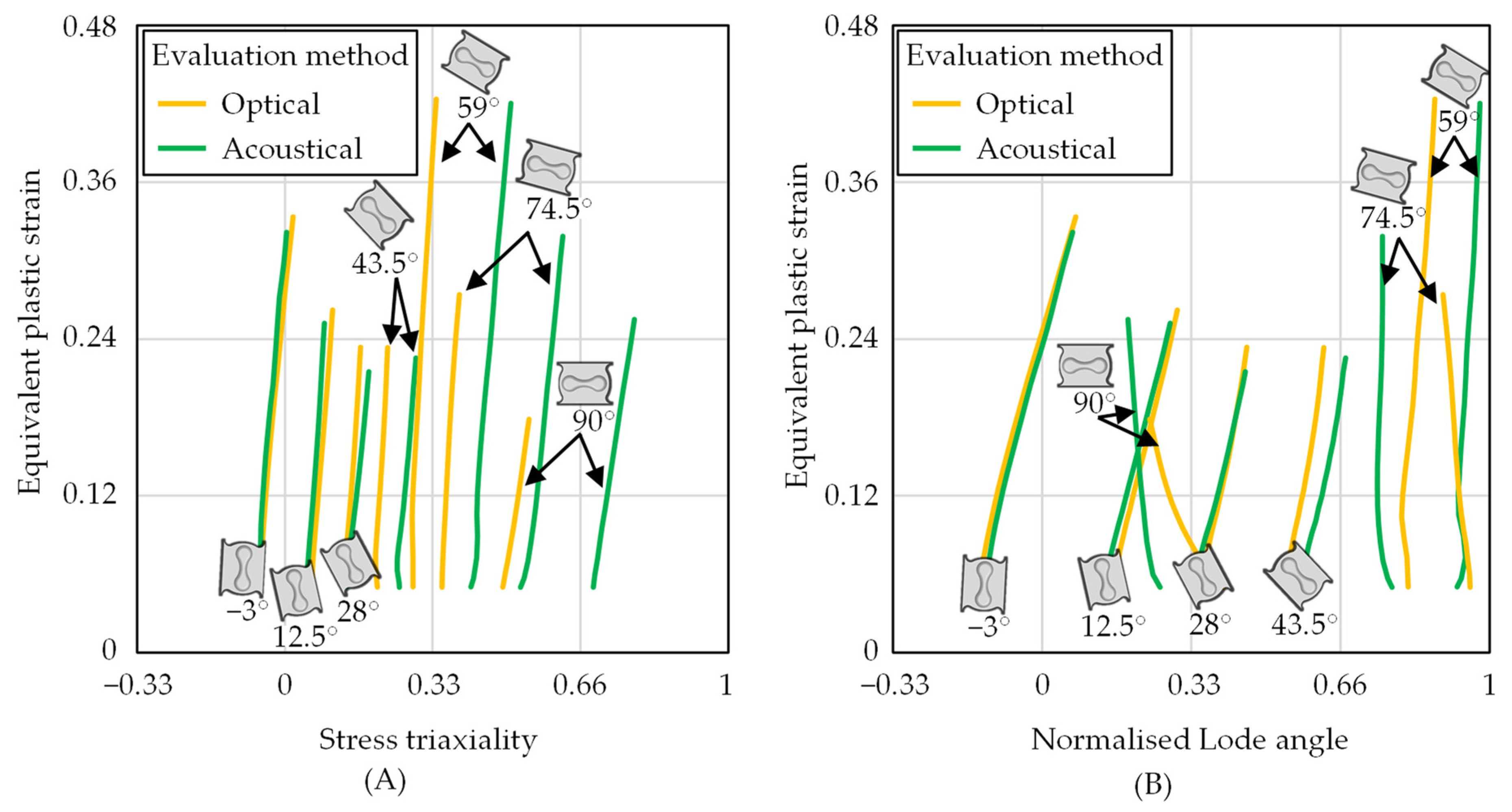
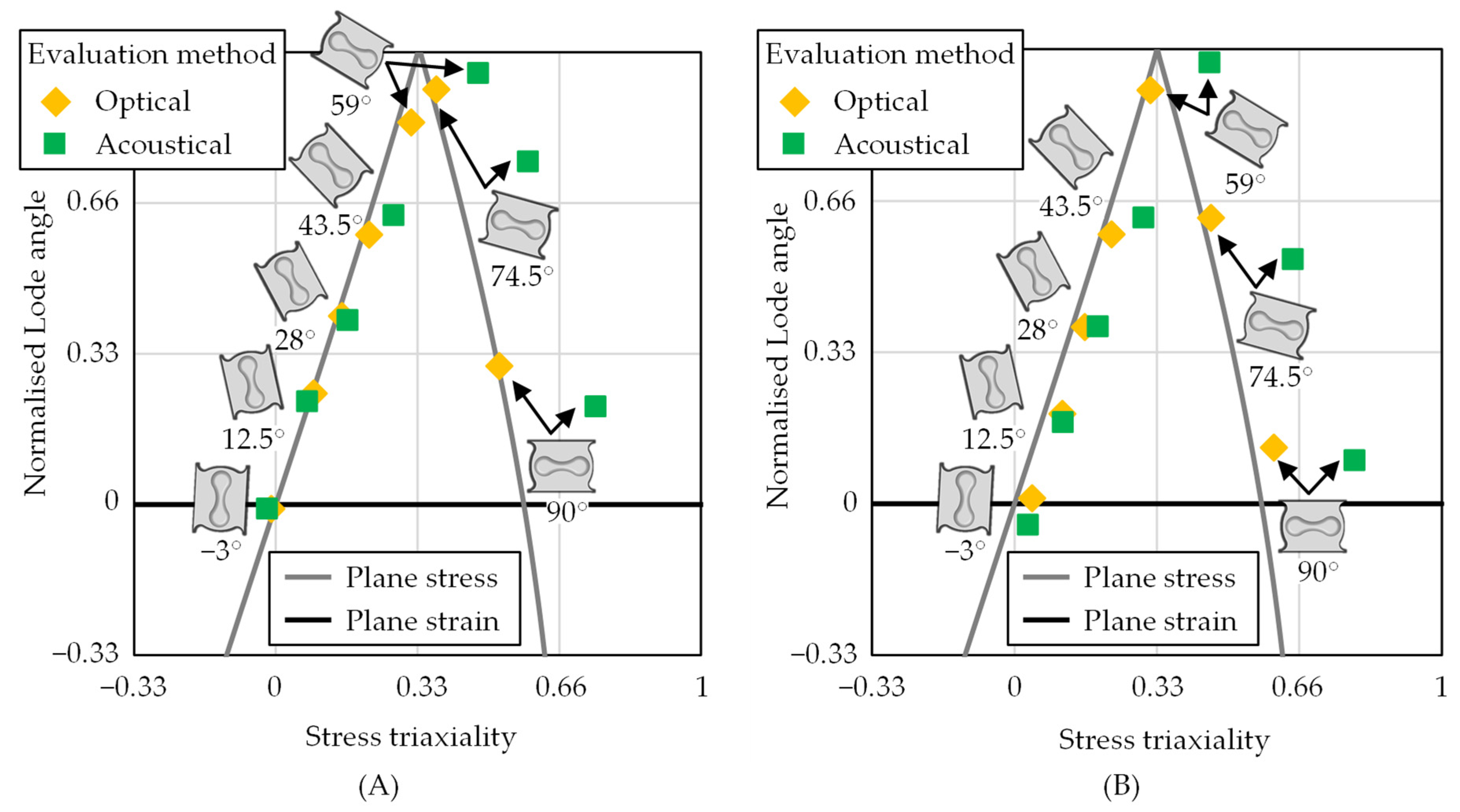
  • For higher loading angles, the characteristic stress states from the acoustical evaluation method are shifted to increased stress triaxialities compared to the optical method.
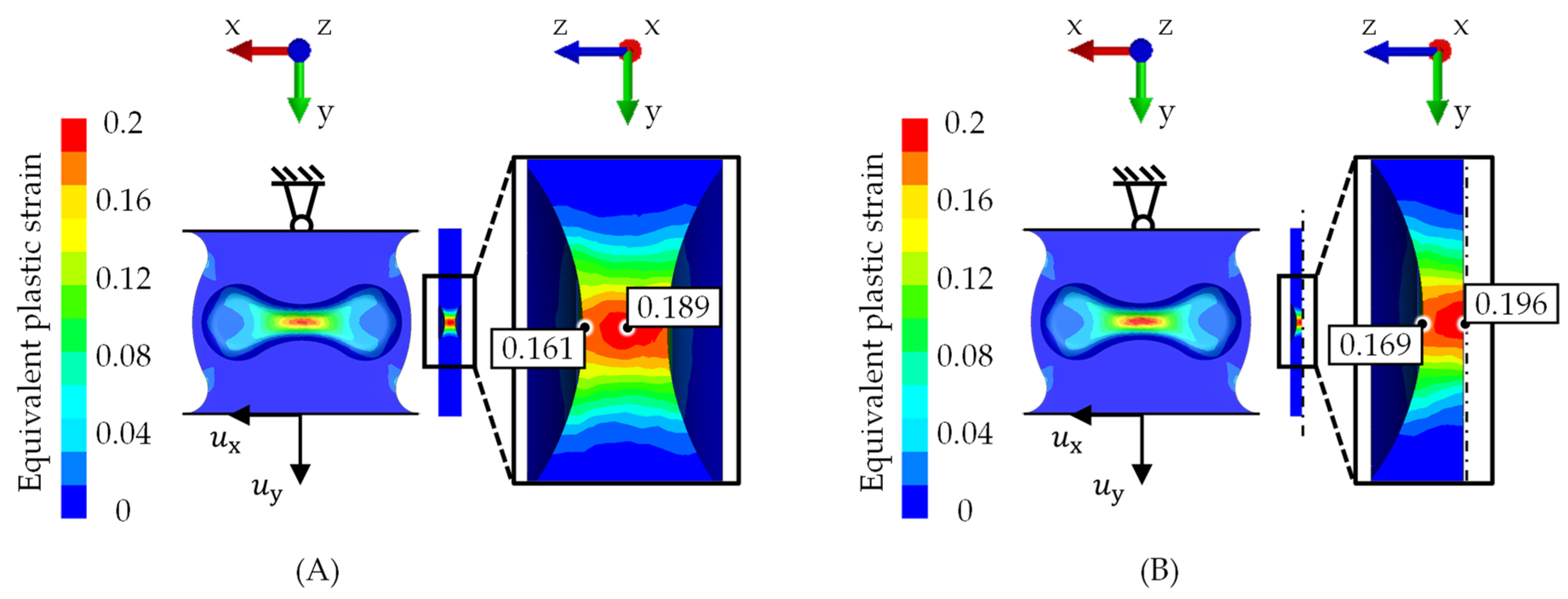
  • The equivalent plastic strain at the fracture shows a gradient over the sheet thickness for higher loading angles, which leads to increased values for the acoustical method.
  • The differences in the characteristic stress state and the fracture strain lead to a steeper development of the optical EMC fracture model than the acoustical model.
  • In a process simulation, the optical EMC fracture model predicted the material fracture too early compared to experimental investigations.
  • Overall, the area where fracture initiation is analysed can have a high impact on fracture modelling depending on the material used and the specimen’s geometry.

Author Contributions

Conceptualization, B.-A.B., H.W. and E.S.; methodology, E.S.; software, E.S.; validation, E.S.; formal analysis, E.S.; investigation, E.S.; resources, B.-A.B. and H.W.; data curation, E.S.; writing—original draft preparation, E.S.; writing—review and editing, B.-A.B. and H.W.; visualization, E.S.; supervision, B.-A.B. and H.W.; project administration, B.-A.B. and H.W.; funding acquisition, B.-A.B. and H.W. All authors have read and agreed to the published version of the manuscript.

Funding

This research was funded by the German Research Foundation (Deutsche Forschungsgemeinschaft, DFG) within the project “Improving the fracture characterisation of advanced high-strength steel sheets by coupling measuring systems for optical forming analysis with acoustic emission technology” with the grant number “385276585”.

Data Availability Statement

The data presented in this study are available on request from the corresponding author. The data are not publicly available due to industrial confidentiality.

Acknowledgments

The authors would like to express gratitude to the company Voestalpine Stahl GmbH for providing the steels, HCT980X and HCT780C, for the experimental investigations. Furthermore, the authors would like to thank H. Vogt from the Institute of Forming Technology and Machines for the support regarding the deep drawing experiments.

Conflicts of Interest

The funders had no role in the design of the study; in the collection, analyses, or interpretation of data; in the writing of the manuscript; or in the decision to publish the results.

References

  1. Fonstein, N. Dual-phase steels. In Automotive Steels—Design, Metallurgy, Processing and Applications; Elsevier: Amsterdam, The Netherlands, 2017; pp. 169–216. [Google Scholar] [CrossRef]
  2. Behrens, B.-A.; Rosenbusch, D.; Wester, H.; Stockburger, E. Material Characterization and Modeling for Finite Element Simulation of Press Hardening with AISI 420C. J. Mater. Eng. Perform. 2022, 31, 825–832. [Google Scholar] [CrossRef]
  3. Behrens, B.-A.; Dröder, K.; Hürkamp, A.; Droß, M.; Wester, H.; Stockburger, E. Finite Element and Finite Volume Modelling of Friction Drilling HSLA Steel under Experimental Comparison. Materials 2021, 14, 5997. [Google Scholar] [CrossRef] [PubMed]
  4. Mohr, D.; Marcadet, S.J. Micromechanically-motivated phenomenological Hosford–Coulomb model for predicting ductile fracture initiation at low stress triaxialities. Int. J. Sol. Struc. 2015, 67–68, 40–55. [Google Scholar] [CrossRef]
  5. Bai, Y.; Wierzbicki, T. Application of extended Mohr–Coulomb criterion to ductile fracture. Int. J. Fract. 2010, 161, 1–20. [Google Scholar] [CrossRef]
  6. Martinez-Gonzalez, E.; Picas, I.; Casellas, D.; Romeu, J. Detection of crack nucleation and growth in tool steels using fracture tests and acoustic emission. Meccanica 2015, 50, 1155–1166. [Google Scholar] [CrossRef]
  7. Behrens, B.-A.; Hübner, S.; Wölki, K. Acoustic Emission—A promising and challenging technique for process monitoring in sheet metal forming. J. Manu Proc. 2017, 29, 281–288. [Google Scholar] [CrossRef]
  8. Shen, G.; Li, L.; Zhang, Z.; Wu, Z. Acoustic Emission Behavior of Titanium During Tensile Deformation. In Advances in Acoustic Emission Technology; Springer: New York, NY, USA, 2015; pp. 235–243. [Google Scholar] [CrossRef]
  9. Murav’ev, T.V.; Zuev, L.B. Acoustic emission during the development of a Lüders band in a low-carbon steel. Tech. Phys. 2008, 53, 1094–1098. [Google Scholar] [CrossRef]
  10. Chuluunbat, T.; Lu, C.; Kostryzhev, A.; Tieu, K. Investigation of X70 line pipe steel fracture during single edge-notched tensile testing using acoustic emission monitoring. Mater. Sci. Eng. A 2015, 640, 471–479. [Google Scholar] [CrossRef]
  11. Panasiuk, K.; Kyziol, L.; Dudzik, K.; Hajdukiewicz, G. Application of the Acoustic Emission Method and Kolmogorov-Sinai Metric Entropy in Determining the Yield Point in Aluminium Alloy. Materials 2020, 13, 1386. [Google Scholar] [CrossRef] [Green Version]
  12. Piñal-Moctezuma, F.; Delgado-Prieto, M.; Romeral-Martínez, L. An acoustic emission activity detection method based on short-term waveform features: Application to metallic components under uniaxial tensile test. Mech. Syst. Signal Process. 2020, 142, 106753. [Google Scholar] [CrossRef] [Green Version]
  13. Petit, J.; Montay, G.; François, M. Strain Localization in Mild (Low Carbon) Steel Observed by Acoustic Emission—ESPI Coupling during Tensile Test. Exp. Mech. 2018, 58, 743–758. [Google Scholar] [CrossRef]
  14. Khamedi, R.; Fallahi, A.; Refahi Oskouei, A. Effect of martensite phase volume fraction on acoustic emission signals using wavelet packet analysis during tensile loading of dual phase steels. Mat. Des. 2010, 31, 2752–2759. [Google Scholar] [CrossRef]
  15. Pathak, N.; Adrien, J.; Butcher, C.; Maire, E.; Worswick, M. Experimental stress state-dependent void nucleation behavior for advanced high strength steels. Int. J. Mech. Sci. 2020, 179, 105661. [Google Scholar] [CrossRef]
  16. DP1000 Voestalpine Steel Division. Data Sheet Dual-Phase Steels. June 2022. Available online: https://www.voestalpine.com/stahl/en/content/download/4523/file/voestalpine_datasheet_dual-phase_steels_EN_20170531.pdf (accessed on 2 May 2023).
  17. CP8000 Voestalpine Steel Division. Data Sheet Complex Phase Steels. October 2022. Available online: https://www.voestalpine.com/stahl/en/content/download/4522/file/voestalpine_datasheet_complexphase_steels_EN_20180711.pdf (accessed on 2 May 2023).
  18. DIN EN ISO 10275:2020; Metallic Materials—Sheet and Strip—Determination of Tensile Strain Hardening Exponent. Beuth: Berlin, Germany, 2020. [CrossRef]
  19. Pelleg, J. Mechanical Testing of Materials. In Mechanical Properties of Materials; Springer: Berlin/Heidelberg, Germany, 2013; pp. 1–84. [Google Scholar] [CrossRef]
  20. DIN EN ISO 10113:2020; Metallic Materials—Sheet and Strip—Determination of Plastic Strain Ratio. Beuth: Berlin, Germany, 2021. [CrossRef]
  21. DIN EN ISO 16808:2022-08; Metallic Materials—Sheet and Strip—Determination of Biaxial Stress-Strain Curve by Means of Bulge Test with Optical Measuring Systems. Beuth: Berlin, Germany, 2022.
  22. Sigvant, M.; Mattiasson, K.; Vegter, H.; Thilderkvist, H. A viscous pressure bulge test for the determination of a plastic hardening curve and equibiaxial material data. Int. J. Mater. Form. 2009, 2, 235–242. [Google Scholar] [CrossRef]
  23. Peshekhodov, I.; Jiang, S.; Vucetic, M.; Bouguecha, A.; Behrens, B.-A. Experimental-numerical evaluation of a new butterfly specimen for fracture characterisation of AHSS in a wide range of stress states. IOP Conf. Ser. Mater. Sci. Eng. 2016, 159, 012015. [Google Scholar] [CrossRef]
  24. Stockburger, E.; Vogt, H.; Wester, H.; Hübner, S.; Behrens, B.-A. Evaluating Material Failure of AHSS Using Acoustic Emission Analysis. Mat. Res. Pro. 2023, 25, 379–386. [Google Scholar] [CrossRef]
  25. Swift, H.W. Plastic instability under plane stress. J. Mech. Phys. Solids 1952, 1, 1–18. [Google Scholar] [CrossRef]
  26. Barlat, F.; Brem, J.C.; Yoon, J.W.; Chung, K.; Dick, R.E.; Lege, D.J.; Pourboghrat, F.; Choi, S.H.; Chu, E. Plane Stress Yield Function for Aluminum Alloy Sheets—Part 1: Theory. Int. J. Plast. 2003, 19, 1297–1319. [Google Scholar] [CrossRef]
  27. Grüner, M.; Merklein, M. Determination of friction coefficients in deep drawing by modification of Siebel’s formula for calculation of ideal drawing force. Prod. Eng. Res. Devel. 2014, 8, 577–584. [Google Scholar] [CrossRef]
  28. Neukamm, F.; Feucht, M.; Haufe, A.; Roll, K. On closing the constitutive gap between forming and crash simulation. In Proceedings of the 10th International LS-DYNA Users Conference, Dearborn, MI, USA, 8–10 June 2008. [Google Scholar]
  29. Heibel, S.; Dettinger, T.; Nester, W.; Clausmeyer, T.; Tekkaya, A.E. Damage Mechanisms and Mechanical Properties of High-Strength Multiphase Steels. Materials 2018, 11, 761. [Google Scholar] [CrossRef] [Green Version]
  30. Pathak, N.; Butcher, C.; Adrien, J.; Maire, E.; Worswick, M. Micromechanical modelling of edge failure in 800 MPa advanced high strength steels. J. Mech. Phys. Solids 2020, 137, 103855. [Google Scholar] [CrossRef]
  31. Bao, Y.; Wierzbicki, T. On fracture locus in the equivalent strain and stress triaxiality space. Int. J. Mech. Sci. 2004, 46, 81–98. [Google Scholar] [CrossRef]
Figure 1. Representation of necking, void formation, and the appearance of a macroscopic crack while forming a tensile specimen.
Jmmp 07 00127 g001
Figure 2. Experimental setup for butterfly tests in a tensile testing machine with optical and acoustical measurement systems.
Jmmp 07 00127 g002
Figure 3. Photograph of the butterfly specimen with magnification of the inner part (A) and achievable stress states by testing butterfly specimen with different loading angles (B).
Jmmp 07 00127 g003
Figure 4. Overview of forming force–amplitude over time measurement from a butterfly specimen (A) and optical as well as acoustic evaluation methods for material fracture (B).
Jmmp 07 00127 g004
Figure 5. Numerical models of the butterfly tests for different loading angles (A) and areas of the optical and acoustic evaluation methods (B).
Jmmp 07 00127 g005
Figure 6. Numerical model (A) and experimental setup (B) of the deep drawing tests.
Jmmp 07 00127 g006
Figure 7. Displacement at fracture in x- as well as y-direction for HCT980X (A) and HCT780C (B) from the butterfly tests with different loading angles.
Jmmp 07 00127 g007
Figure 8. Comparison of the full (A) and half model (B) of the butterfly test for a loading angle of 90°.
Jmmp 07 00127 g008
Figure 9. Comparison of the equivalent plastic strain from digital image correlation (DIC) as well as from the numerical models (FEA) of the butterfly specimen for HCT980X (A) and HCT780C (B).
Jmmp 07 00127 g009
Figure 10. Equivalent plastic strain triaxiality (A) and equivalent plastic-strain-normalised Lode angle curves (B) of the butterfly specimens for different loading angles of HCT980X.
Jmmp 07 00127 g010
Figure 11. Characteristic stress state of the butterfly specimens for different loading angles of HCT980X (A) and HCT780C (B).
Jmmp 07 00127 g011
Figure 12. Comparison of the fracture strain for the butterfly specimen from the optical and the acoustic evaluation methods of HCT980X (A) and HCT780C (B).
Jmmp 07 00127 g012
Figure 13. Comparison of the equivalent plastic strain over the sheet thickness of the butterfly specimen for HCT980X.
Jmmp 07 00127 g013
Figure 14. Three-dimensional plot of the EMC fracture models from the optical and acoustic evaluation methods for HCT980X (A) and HCT780C (B).
Jmmp 07 00127 g014
Figure 15. Damage variable plot of the deep drawing simulation for the optical (top) as well as the acoustic (middle) EMC fracture model compared to the experimental deep drawing component (bottom) for HCT980X (A) and HCT780C (B).
Jmmp 07 00127 g015
Figure 16. Stress state development and plane stress state of the failed element from the B-pillar simulation for HCT980X (A) and HCT780C (B).
Jmmp 07 00127 g016
Table 1. Chemical composition in mass % of the used HCT980X and HCT780C from spark spectroscopy.
ElementCSiMnPSAlCr + MoTi + NbBVFe
HCT980X0.1390.1861.5620.0210.0030.2410.8440.0530.00050.02Bal.
HCT780C0.1020.2061.8470.0220.0020.1970.7840.06950.00040.08Bal.
Table 2. Mechanical properties, parameters of the yield curve YLD2000, and parameters of the extrapolation approach according to Swift.
Parameter R p , 0.2   in   MPa R m   in   MPa A g   in   % A 80   in   % r 0 r 45 r 90
HCT980X747.31052.47.4311.870.9041.0411.068
HCT780C629.2809.79.5316.580.8841.0940.949
Parameter k f , 0   in MPa k f , 45   in MPa k f , 90   in MPa l S   in MPa   m S   n S
HCT980X757.3742.2743.613797.16 × 10−47.97 × 10⁻²
HCT780C631.4622.7605.8112321.65 × 10−410.57 × 10⁻²
Disclaimer/Publisher’s Note: The statements, opinions and data contained in all publications are solely those of the individual author(s) and contributor(s) and not of MDPI and/or the editor(s). MDPI and/or the editor(s) disclaim responsibility for any injury to people or property resulting from any ideas, methods, instructions or products referred to in the content.

