
Evaluation of Additively-Manufactured Internal Geometrical Features Using X-ray-Computed Tomography
 , , , and
Abstract
:1. Introduction
2. Materials and Methods
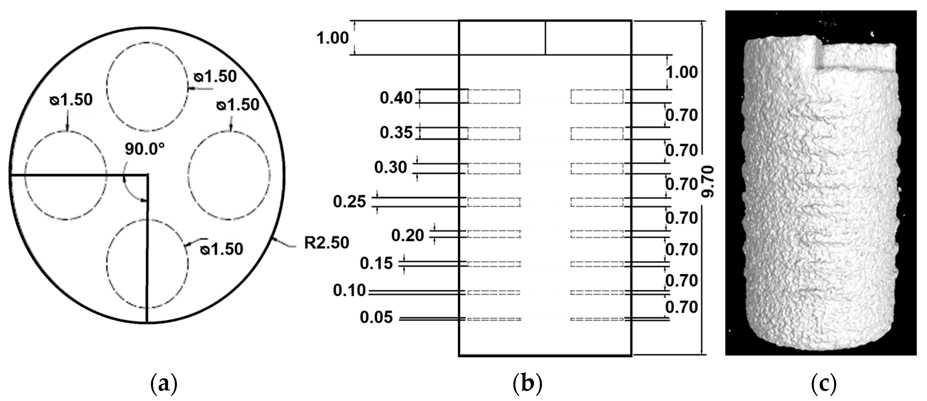
2.1. Samples
2.2. Manufacturing Processes
2.3. CT Measurement
2.4. Metrological Evaluation
2.4.1. Voxel Data Filter
2.4.2. Surface Determination
2.4.3. Coordinate Measurement Functions
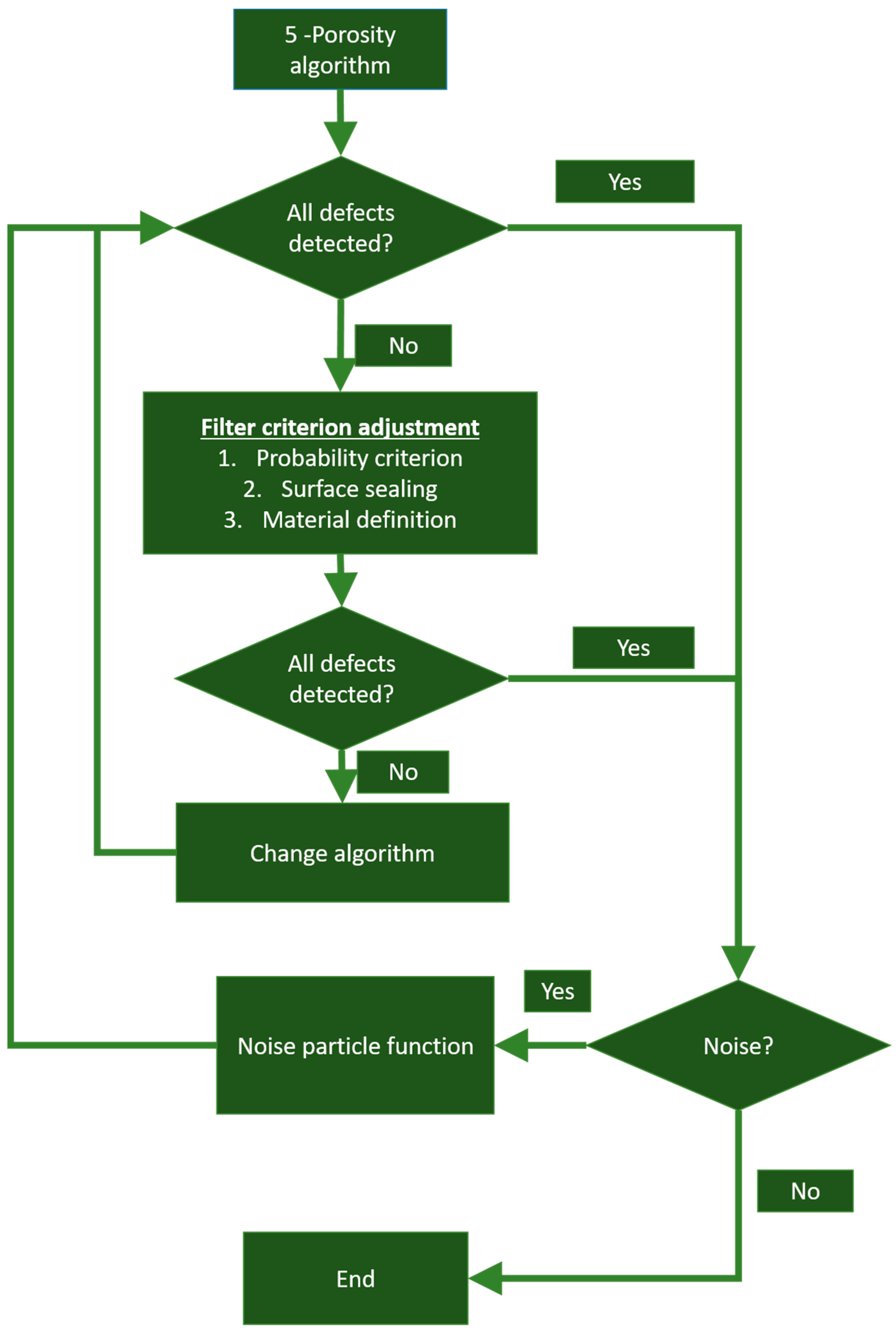
2.5. Porosity Analysis
3. Results
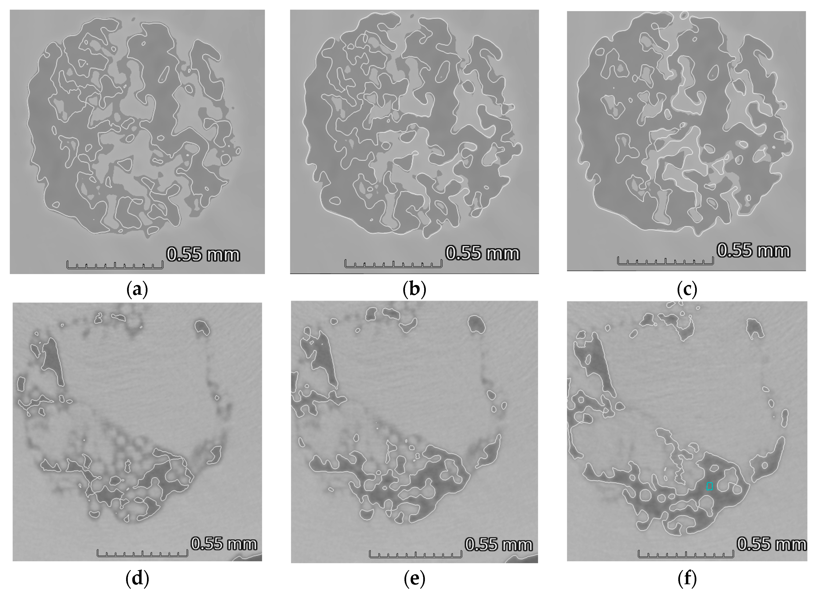
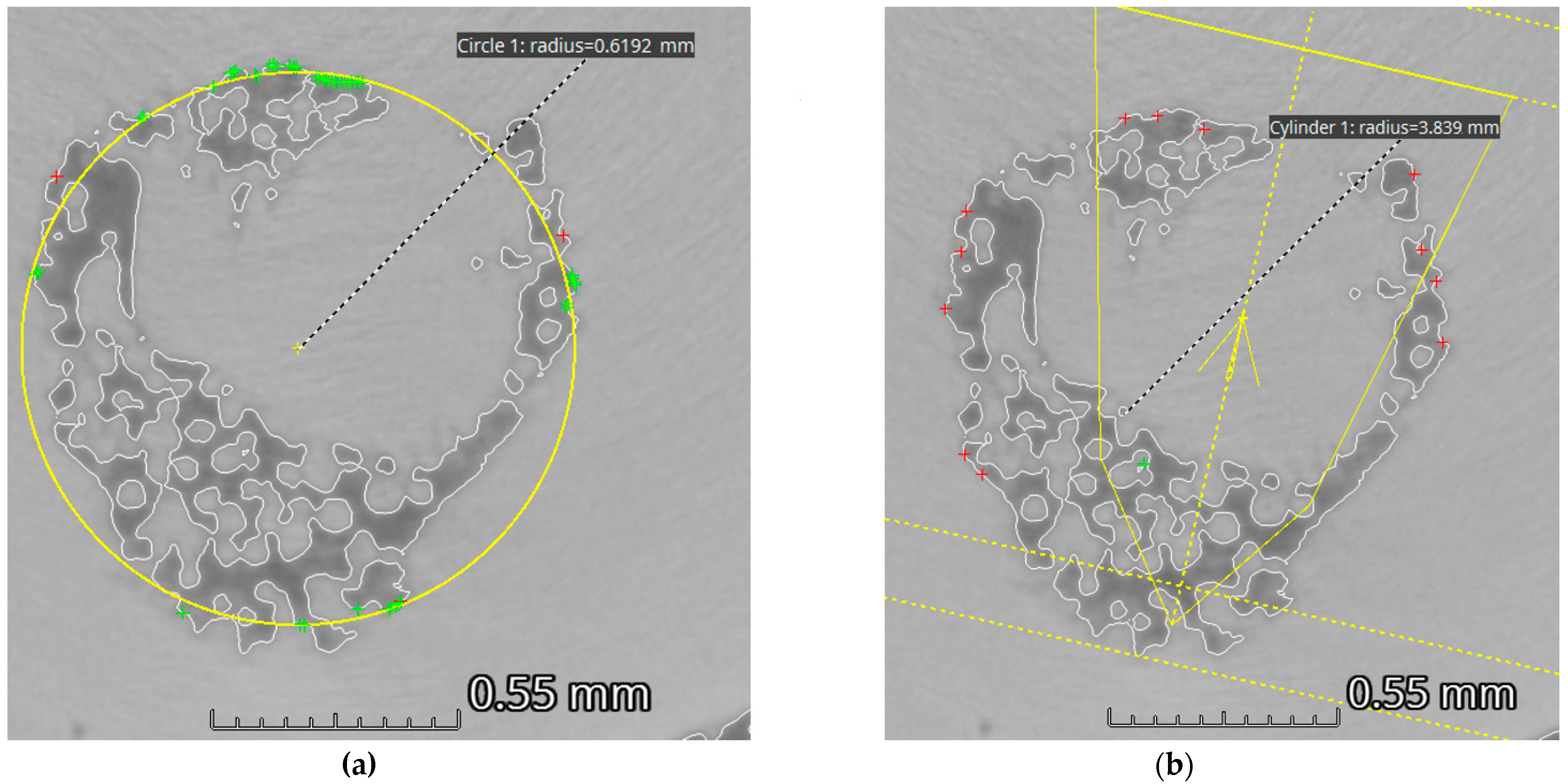
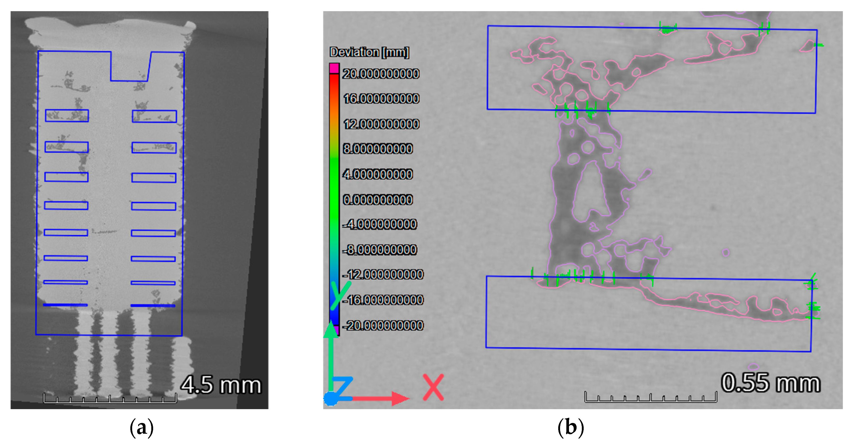
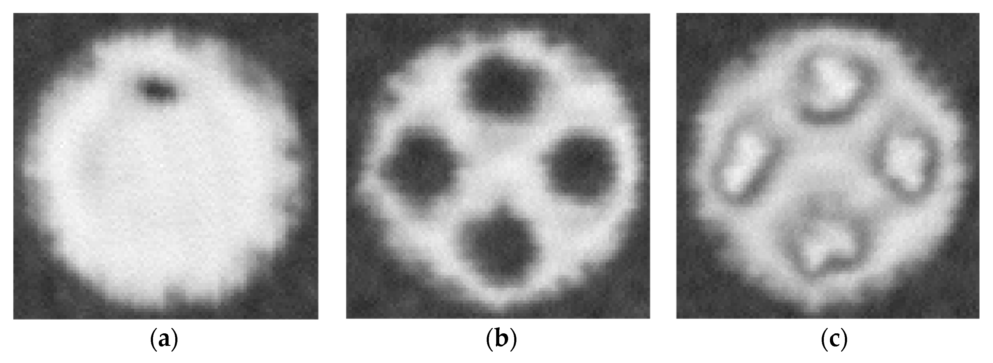
3.1. Metrological Evaluation
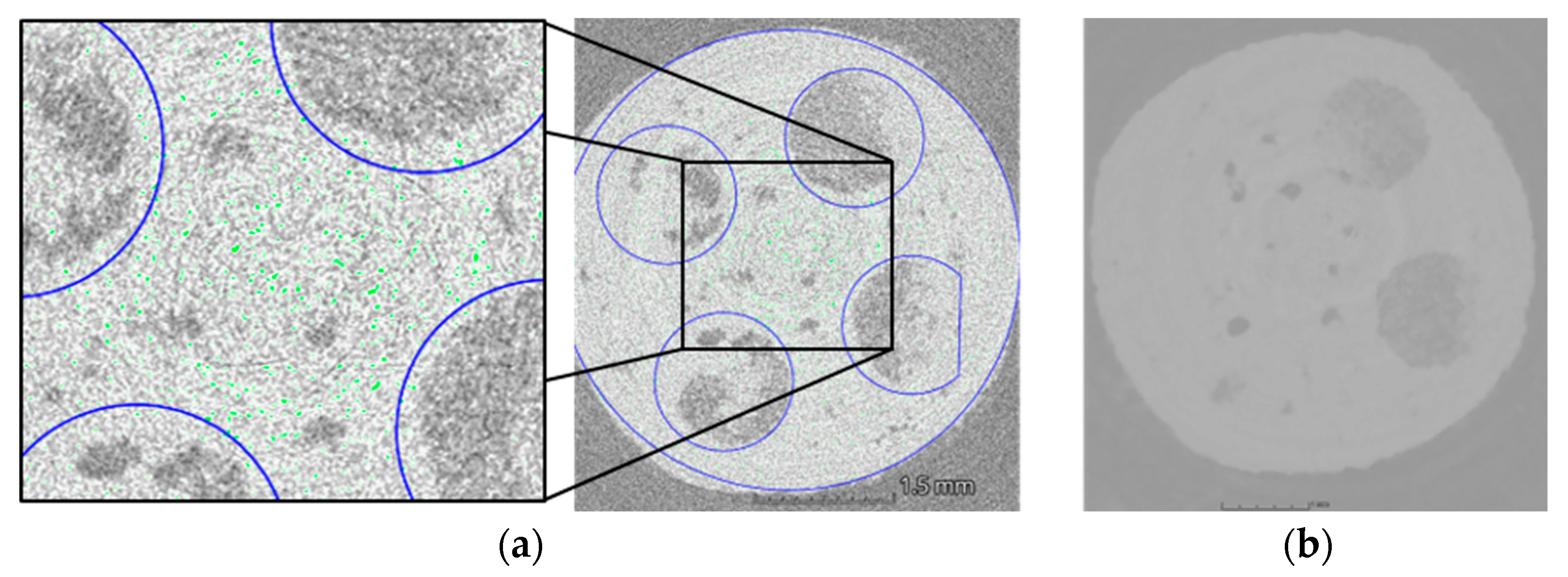
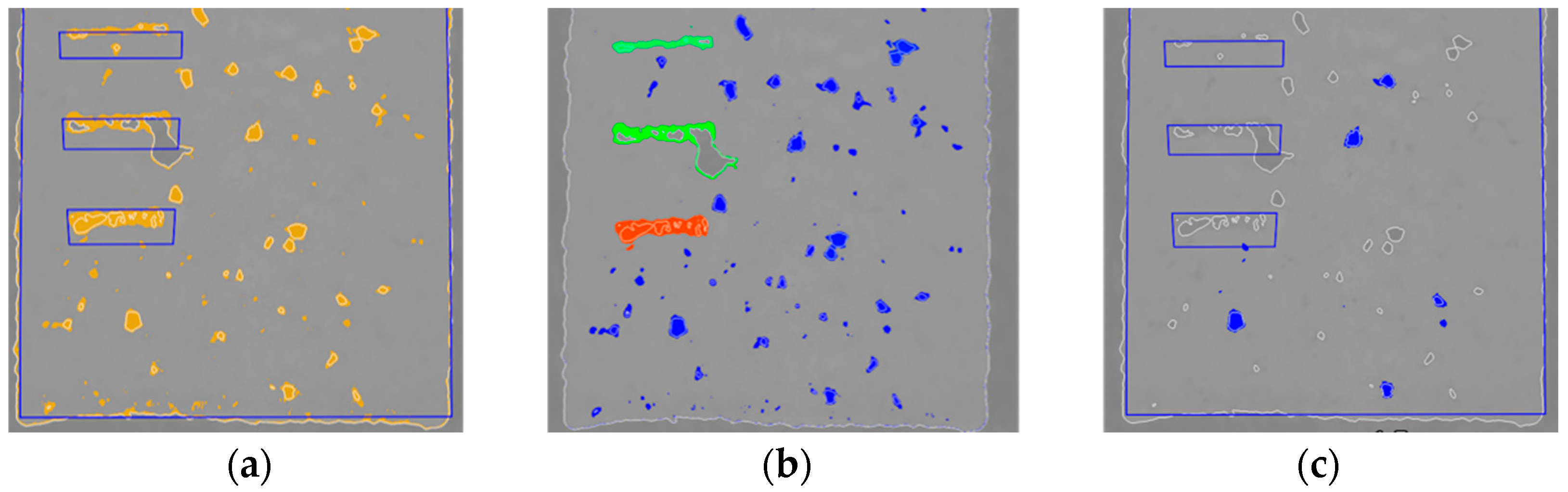
3.2. Volume Filtering
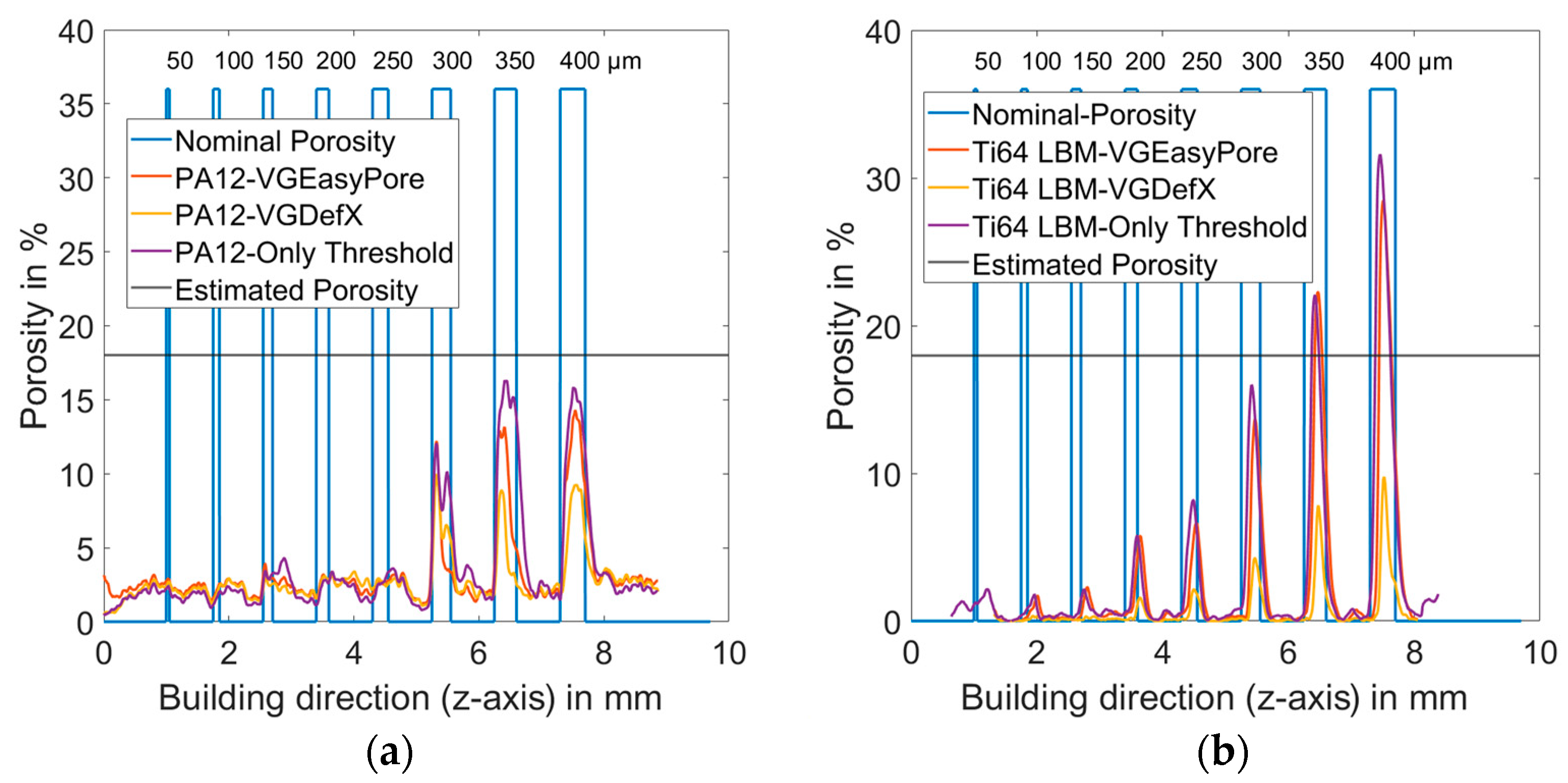
Porosity Analysis
4. Discussion
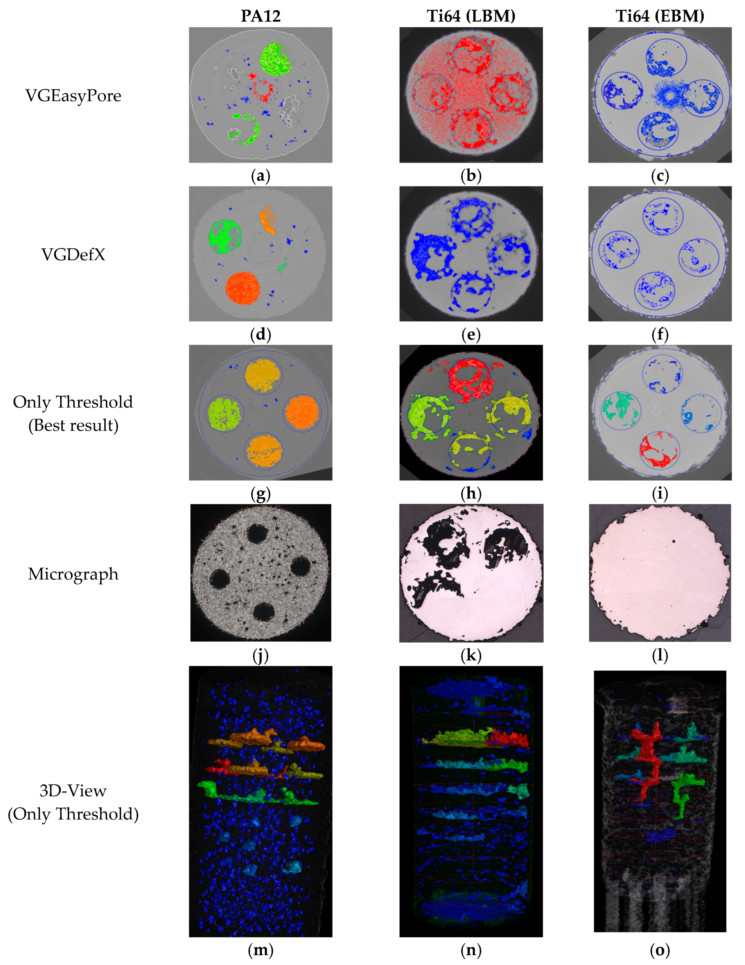
4.1. VGEasyPore
4.2. VGDefX
4.3. Only Threshold-Method
4.4. Evaluating the Porosity Measurement
5. Conclusions
5.1. Recommendation for Metrolocigal Assessment with CT
- Without going further into the CT scan, a volume filtering method like the non-local means method was considered a useful tool with which to prepare the volume data for surface determination, since the transition between material and background/defects could be improved.
- Regarding surface determination, the transition between the material and internal defects was influenced by the chosen method of calculation. Although optimization of the transition could be achieved using an ROI-based iterative surface determination with the mean gray value of an internal defect, better replicability could be accomplished with an automatic calculation of the mean value of the background peak.
- Based on the differences in surface determinations, the evaluation should be performed without the use of the surface determination as a starting point for the porosity algorithm.
5.2. Recommendations on the Procedure for Measuring Internal Structures
- Reduce the filter criterions e.g., the material threshold to add internal defects to the analyzing area.
- Disable filtering of the results due to AI. Automatically estimating or manually setting the threshold value can influence the detectable volume and shape of the internal structures and noise. The probability criterion must be set to 0.
- Close surface-connected defects.
Author Contributions
Funding
Data Availability Statement
Acknowledgments
Conflicts of Interest
References
- Klahn, C.; Leutenecker, B.; Meboldt, M. Design for Additive Manufacturing—Supporting the Substitution of Components in Series Products. Procedia CIRP 2014, 21, 138–143. [Google Scholar] [CrossRef]
- Blakey-Milner, B.; Gradl, P.; Snedden, G.; Brooks, M.; Pitot, J.; Lopez, E.; Leary, M.; Berto, F.; Du Plessis, A. Metal additive manufacturing in aerospace: A review. Mater. Des. 2021, 209, 110008. [Google Scholar] [CrossRef]
- Villarraga-Gómez, H.; Peitsch, C.; Ramsey, A.; Smith, S. The Role of Computed Tomography in Additive Manufacturing. Am. Soc. Precis. Eng. 2018, 69, 201–209. [Google Scholar]
- Du Plessis, A.; Yadroitsava, I.; Yadroitsev, I. Effects of defects on mechanical properties in metal additive manufacturing: A review focusing on X-ray tomography insights. Mater. Des. 2020, 187, 108385. [Google Scholar] [CrossRef]
- Tammas-Williams, S.; Withers, P.J.; Todd, I.; Prangnell, P.B. The Influence of Porosity on Fatigue Crack Initiation in Additively Manufactured Titanium Components. Sci. Rep. 2017, 7, 7308. [Google Scholar] [CrossRef]
- Zhang, L.; Lifton, J.; Hu, Z.; Hong, R.; Feih, S. Influence of geometric defects on the compression behaviour of thin shell lattices fabricated by micro laser powder bed fusion. Addit. Manuf. 2022, 58, 103038. [Google Scholar] [CrossRef]
- Gapinski, B.; Wieczorowski, M.; Grzelka, M.; Arroyo Alonso, P.; Bermudez Tome, A. The application of micro computed tomography to assess quality of parts manufactured by means of rapid prototyping. Polimery 2017, 62, 53–59. [Google Scholar] [CrossRef]
- Du Plessis, A.; Yadroitsava, I.; Yadroitsev, I.; Le Roux, S. X-Ray microcomputed tomography in additive manufacturing: A review of current technology and applications. 3D Print. Addit. Manuf. 2018, 5, 3. [Google Scholar] [CrossRef]
- Cersullo, N.; Mardaras, J.; Emile, P.; Nickel, K.; Holzinger, V.; Hühne, C. Effect of Internal Defects on the Fatigue Behavior of Additive Manufactured Metal Components: A Comparison between Ti6Al4V and Inconel 718. Materials 2022, 15, 6882. [Google Scholar] [CrossRef]
- Masuo, H.; Tanaka, Y.; Morokoshi, S.; Yagura, H.; Uchida, T.; Yamamoto, Y.; Murakami, Y. Effects of Defects, Surface Roughness and HIP on Fatigue Strength of Ti-6Al-4V manufactured by Additive Manufacturing. Procedia Struct. Integr. 2017, 7, 19–26. [Google Scholar] [CrossRef]
- Gates, N.; Fatemi, A. Friction and roughness induced closure effects on shear-mode crack growth and branching mechanisms. Int. J. Fatigue 2016, 92, 442–458. [Google Scholar] [CrossRef]
- Caillé, J.-M.; Salamon, G. (Eds.) Computerized Tomography; Springer: Berlin/Heidelberg, Germany, 1980. [Google Scholar]
- Lifton, J.; Bakar, A.A.; Tan, J.T.; Malcolm, A. Internal Surface Roughness Measurement of Metal AM Channels via X-ray Computed Tomography: A Case Study. In Proceedings of the Singapore International NDT Conference & Exhibition, (SINCE 2022), Singapore, 7–8 November 2022. [Google Scholar]
- Iassonov, P.; Gebrenegus, T.; Tuller, M. Segmentation of X-ray computed tomography images of porous materials: A crucial step for characterization and quantitative analysis of pore structures. Water Resour. Res. 2009, 45, W09415. [Google Scholar] [CrossRef]
- Jaques, V.A.J.; Du Plessis, A.; Zemek, M.; Šalplachta, J.; Stubianová, Z.; Zikmund, T.; Kaiser, J. Review of porosity uncertainty estimation methods in computed tomography dataset. Meas. Sci. Technol. 2021, 32, 122001. [Google Scholar] [CrossRef]
- Villarraga-Gómez, H.; Lee, C.; Smith, S.T. Dimensional metrology with X-ray CT: A comparison with CMM measurements on internal features and compliant structures. Precis. Eng. 2018, 51, 291–307. [Google Scholar] [CrossRef]
- Rezaei, F.; Izadi, H.; Memarian, H.; Baniassadi, M. The effectiveness of different thresholding techniques in segmenting micro CT images of porous carbonates to estimate porosity. J. Pet. Sci. Eng. 2019, 177, 518–527. [Google Scholar] [CrossRef]
- Du Plessis, A.; Le Roux, S.G.; Waller, J.; Sperling, P.; Achilles, N.; Beerlink, A.; Métayer, J.-F.; Sinico, M.; Probst, G.; Dewulf, W.; et al. Laboratory X-ray tomography for metal additive manufacturing: Round robin test. Addit. Manuf. 2019, 30, 100837. [Google Scholar] [CrossRef]
- Abera, K.A.; Manahiloh, K.N.; Nejad, M. The effectiveness of global thresholding techniques in segmenting two-phase porous media. Constr. Build. Mater. 2017, 142, 256–267. [Google Scholar] [CrossRef]
- Payel, R.; Saurab, D.; Nilanjan, D.; Gaotami, D.; Sayan, C.; Ruben, R. Adaptive thresholding: A comparative Study. In Proceedings of the 2014 International Conference on Control, Instrumentation, Communication and Computational Technologies (ICCICCT), Kanyakumari District, India, 10–11 July 2014; IEEE: Piscataway, NJ, USA, 2014. [Google Scholar]
- ASTM E1570-11; Standard Practice for Computed Tomographic (CT) Examination. ASTM International: West Conshohocken, PA, USA, 2011.
- Bäreis, J.; Semjatov, N.; Renner, J.; Ye, J.; Zongwen, F.; Körner, C. Electron-optical in-situ crack monitoring during electron beam powder bed fusion of the Ni-Base superalloy CMSX-4. Prog. Addit. Manuf. 2022, 7, 1–6. [Google Scholar] [CrossRef]
- ZEISS. ZEISS CT Cookbook-English Edition: Best Practice Guide for ZEISS METROTOM Settings; ZEISS: Jena, Germany; Available online: https://shop.metrology.zeiss.de/INTERSHOP/web/WFS/IMT-DE-Site/de_DE/-/EUR/ViewProduct-Start?SKU=600033-2022-016&CategoryName=240100&CatalogID=200000&ExtendedNavigation=true (accessed on 15 March 2023).
- Bellens, S.; Vandewalle, P.; Dewulf, W. Deep learning based porosity segmentation in X-ray CT measurements of polymer additive manufacturing parts. Procedia CIRP 2021, 96, 336–341. [Google Scholar] [CrossRef]
- Feldkamp, J.A.; Davis, J.C.; Kress, J.W. Practical cone-beam algortihm. J. Opt. Soc. Am. 1984, 1, 612–619. [Google Scholar] [CrossRef]
- Mahmoudi, M.; Sapiro, G. Fast image and video denoising via nonlocal means of similar neighborhoods. IEEE Signal Process. Lett. 2005, 12, 839–842. [Google Scholar] [CrossRef]
- Otsu, N. A Threshold Selection Method from Gray-Level Histograms. IEEE Trans. Syst. Man Cybern. 1979, 9, 62–66. [Google Scholar] [CrossRef]
- Kittler, J.; Illingworth, J. Minimum Error Thresholding. Pattern Recognit. 1986, 19, 41–47. [Google Scholar] [CrossRef]
- Cho, S.; Haralick, R.; Yi, S. Improvement of kittler and illingworth’s minimum error thresholding. Pattern Recognit. 1989, 22, 609–617. [Google Scholar] [CrossRef]
- Buades, A.; Coll, B.; Morel, J.-M. A Non-Local Algorithm for Image Denoising. In Proceedings of the 2005 IEEE Computer Society Conference on Computer Vision and Pattern Recognition (CVPR’05), San Diego, CA, USA, 20–26 June 2005; IEEE: Piscataway, NJ, USA, 2005; pp. 60–65, ISBN 0-7695-2372-2. [Google Scholar]
- Bundesverband der Deutschen Gießerei-Industrie e.V. BDG. BDG-Richtlinie P203: Porositätsanalyse und -Beurteilung Mittels Industrieller Röntgen-Computertomographie (CT); Bundesverband der Deutschen Gießerei-Industrie e.V. BDG: Düsseldorf, Germany, 2019. [Google Scholar]
- DIN EN ISO 1183-3:2000-05; Kunststoffe—Bestimmung der Dichte von Nicht Verschäumten Kunststoffen—Teil 3: Gas-Pyknometer-Verfahren. Beuth Verlag: Berlin, Germany, 2000; 83.080.01. [CrossRef]


| EBM | LBM | LBP | ||
|---|---|---|---|---|
| Material | Unit | Ti64 | Ti64 | PA12 |
| Machine | Research System | Aconity Mini | Research System | |
| Beam Power | W | 210 | 900 | 16 |
| Beam diameter | µm | 250 | 90 | 500 |
| Scanning speed | mm s−1 | 1200 | 1200 | 2000 |
| Hatch line spacing | µm | 100 | 120 | 200 |
| Layer thickness | µm | 50 | 50 | 100 |
| Unit | Ti64 (EBM) | Ti64 (LBM) | PA12 | |
|---|---|---|---|---|
| VGEasyPore | ||||
| Threshold | Abs./Est. | Abs./Est. | Abs./Est. | |
| Probability Threshold | 0 | 0 | 0 | |
| VGDefX | ||||
| Material Definition | Surface Det. | Surface Det. | Surface Det. | |
| Threshold Deviation | σ | −1 | −1 | −1 |
| Probability Threshold | 0 | 0 | 0 | |
| Surface Sealing | vx | On/0 | On/0 | On/0 |
| Only Threshold | ||||
| Material Definition | Surface Det. | Surface Det. | Surface Det. | |
| Threshold | manually | manually | manually | |
| Probability criterion | 0 | 0 | 0 |
| EBM | LBM | LBP | ||
|---|---|---|---|---|
| Method | Unit | Ti64 | Ti64 | PA12 |
| Micrograph/ELO | % | 0 | 15.85 | 34.01 |
| ELO | % | 22.23 | / | / |
| VGEasyPore | % | 7.15 | 14.23 | 28.02 |
| VGDefX | % | 9.31 | 11.75 | 9.71 |
| Only Threshold | % | 7.12 | 15.73 | 31.12 |
| Sample density | ||||
| Pycnometry | g/cm3 | 4.4323 | 4.4164 | 1.0008 |
| VGEasyPore | g/cm3 | 4.5206 | 4.4659 | 1.4556 |
| VGDefX | g/cm3 | 4.5206 | 4.4087 | 1.4750 |
| Only Threshold | g/cm3 | 4.4196 | 4.4909 | 1.4303 |
| Sample weight | g | 0.8955 | 0.8219 | 0.2715 |
Disclaimer/Publisher’s Note: The statements, opinions and data contained in all publications are solely those of the individual author(s) and contributor(s) and not of MDPI and/or the editor(s). MDPI and/or the editor(s) disclaim responsibility for any injury to people or property resulting from any ideas, methods, instructions or products referred to in the content. |
© 2023 by the authors. Licensee MDPI, Basel, Switzerland. This article is an open access article distributed under the terms and conditions of the Creative Commons Attribution (CC BY) license (https://creativecommons.org/licenses/by/4.0/).
Share and Cite
Baumgärtner, B.; Rothfelder, R.; Greiner, S.; Breuning, C.; Renner, J.; Schmidt, M.; Drummer, D.; Körner, C.; Markl, M.; Hausotte, T. Evaluation of Additively-Manufactured Internal Geometrical Features Using X-ray-Computed Tomography. J. Manuf. Mater. Process. 2023, 7, 95. https://doi.org/10.3390/jmmp7030095
Baumgärtner B, Rothfelder R, Greiner S, Breuning C, Renner J, Schmidt M, Drummer D, Körner C, Markl M, Hausotte T. Evaluation of Additively-Manufactured Internal Geometrical Features Using X-ray-Computed Tomography. Journal of Manufacturing and Materials Processing. 2023; 7(3):95. https://doi.org/10.3390/jmmp7030095
Chicago/Turabian StyleBaumgärtner, Benjamin, Richard Rothfelder, Sandra Greiner, Christoph Breuning, Jakob Renner, Michael Schmidt, Dietmar Drummer, Carolin Körner, Matthias Markl, and Tino Hausotte. 2023. "Evaluation of Additively-Manufactured Internal Geometrical Features Using X-ray-Computed Tomography" Journal of Manufacturing and Materials Processing 7, no. 3: 95. https://doi.org/10.3390/jmmp7030095