Systematic Approach for Investigating Temporal Variability in Production Systems to Improve Production Planning and Control

Abstract

Including the inherent temporal variability in a production system in planning and control processes can ensure the fulfillment of the production schedule and increase key performance indicators. This benefits the sustainable and efficient use of the system. The current lack of consideration of this inherent temporal variability in production planning leads to optimistic estimates and calculations of planned values that cannot be met. To complete this information, the inherent temporal variability in a production system is investigated using a systematic approach. This approach detects, identifies, and quantifies inherent temporal variability and is applied to a data base created via an automated, event-driven procedure. The approach is tested in a smart factory laboratory. The results to date on improving production planning and control are promising as key performance indicators have been increased. There is still a need for action to ensure the fulfillment of the production schedule. Concluding, work on this topic has just begun, as can be seen from the discussion section. More data need to be collected and aggregated for future research. This publication is intended to motivate researchers to address this issue and better manage the existing uncertainty in production through the use of data.

1. Introduction

This research project presents aims to improve production planning and control by investigating the inherent temporal variability in a production system. The production run at the operational level with regard to the realization of the production schedule is considered. The production schedule is created via production planning and realized through production control. Several production subjects—humans, machines, materials, systems, tools, etc.—are involved in the realization of the production schedule. Each subject can be a trigger of events that influence the fulfillment of the production schedule.

The events can be planned or unplanned. As examples, there are random, unforeseeable events such as machine breakdowns, sudden rush jobs, rework, staff absences due to illness, or unplanned material shortages [1] (p. 265) [2,3]. In addition, there are deliberately provoked events such as product variety, lot/batch sizing, setup, manufacturing layout, planned maintenance, or engineering processes [1] (p. 265) [2,3]. The events, in turn, trigger planned or unplanned operations as well as influencing planned operations in terms of time. Events that trigger unplanned operations or influence planned operations in terms of time cause temporal variability.

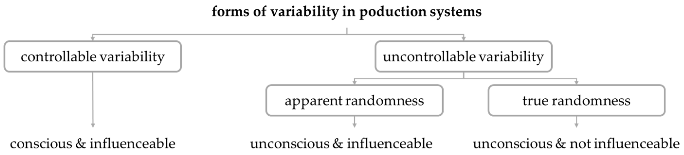
The National Institute of Standards and Technology (NIST) has generally divided variability into two forms:

• Controllable variability;
• Uncontrollable variability.

Controllable variability is defined by a stable and consistent pattern of variation over time [4]. In terms of events, controllable variability is the result of conscious decisions [1] (p. 265). Their causes are deterministic. Uncontrollable variability is characterized by a pattern of variation that changes over time and can therefore be unpredictable [4]. Stochastic events that cause uncontrollable variability are consequently beyond the control range [1] (p. 265). According to Hopp and Spearman, uncontrollable variability is the result of randomness, of which there are at least two types: apparent and true randomness. The presence of randomness is due to missing or incomplete information. An overview of the forms of variability in production environments is given in Figure 1.

Events of apparent and true randomness are unconscious. The difference is in the influenceability. Events of apparent randomness can be influenced, whereas events of true randomness cannot [1] (pp. 265–266).

The triggered operations, whether planned or unplanned, claim production time, so each operation must be considered in production planning if reliable planned values are to be determined. Therefore, the events that occur should be conscious and influenceable. Unfortunately, the sum of events that continuously affect a production system as well as their partially unpredictable occurrence behavior is not conscious and influenceable, so they are not all considered in the original schedule [2]. As a result, production schedules cannot be met due to excessively long lead times or throughput losses [5].

Existing approaches to production scheduling and its optimization involve mathematical models that first map the total capacity load of the production system. Subsequently, the production jobs are distributed among the capacities in such a way that a maximum output quantity is achieved at a minimum cost. The calculation factors are made up of the capacity of the production units, the demand of a time period, the capacity load caused by the job, storage cost rates, delivery dates, and so on [6] (p. 13). The inherent temporal variability in the production system is not part of the calculation formula, resulting in optimistic planned values. Another missing component in the formulas is penalty costs due to missed deadlines or costs for additional capacity to correct shortfalls.

Deviations between the actual and planned values in production scheduling are an integral part of the production process, as described in the norms and standards of the VDMA [7] (p. 9). The assumption for the continued existence of deviations is incomplete planning data. The incompleteness of the data is caused by the lack of consideration of the system’s inherent temporal variability. Inherent, herein, means that something is an integral part and cannot be removed. Surprisingly, the data necessary to consider inherent temporal variability may already exist. Today, production systems generate a lot of unused data [8] (p. 24). Unused data have no value [8] (p. 24). It is known that the data generated by intelligent production systems hold far more potential for improving production planning and control than is currently being exploited [8] (p. 24).

Romero-Silva, R. et al. offer a summary of numerous research papers on the topic of ‘variability in production systems’ from recent years. A key message of the summary is the lack of metrics to directly assess the impacts of the numerous variability factors on the overall performance of a production system [9].

In the publication by Dequeant, K. et al., an overview of the causes of variability in production systems in the semiconductor industry is given. They complete the explanations with methods for eliminating the causes if these causes are known. They also highlight the negative impact of variability on lead time, capacity, and system resilience. The authors note that more information is needed to fully understand production systems, including about variability, which is becoming increasingly possible due to technological advances [10].

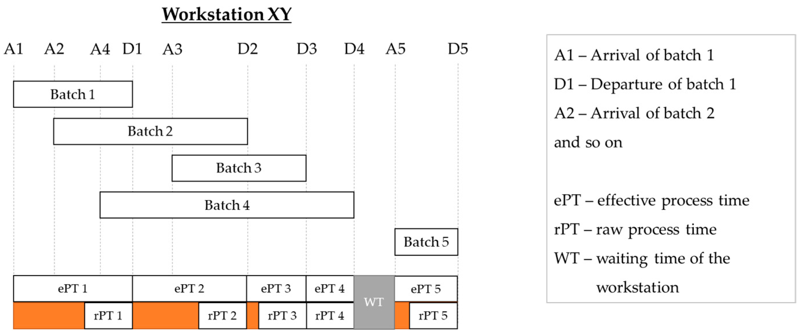
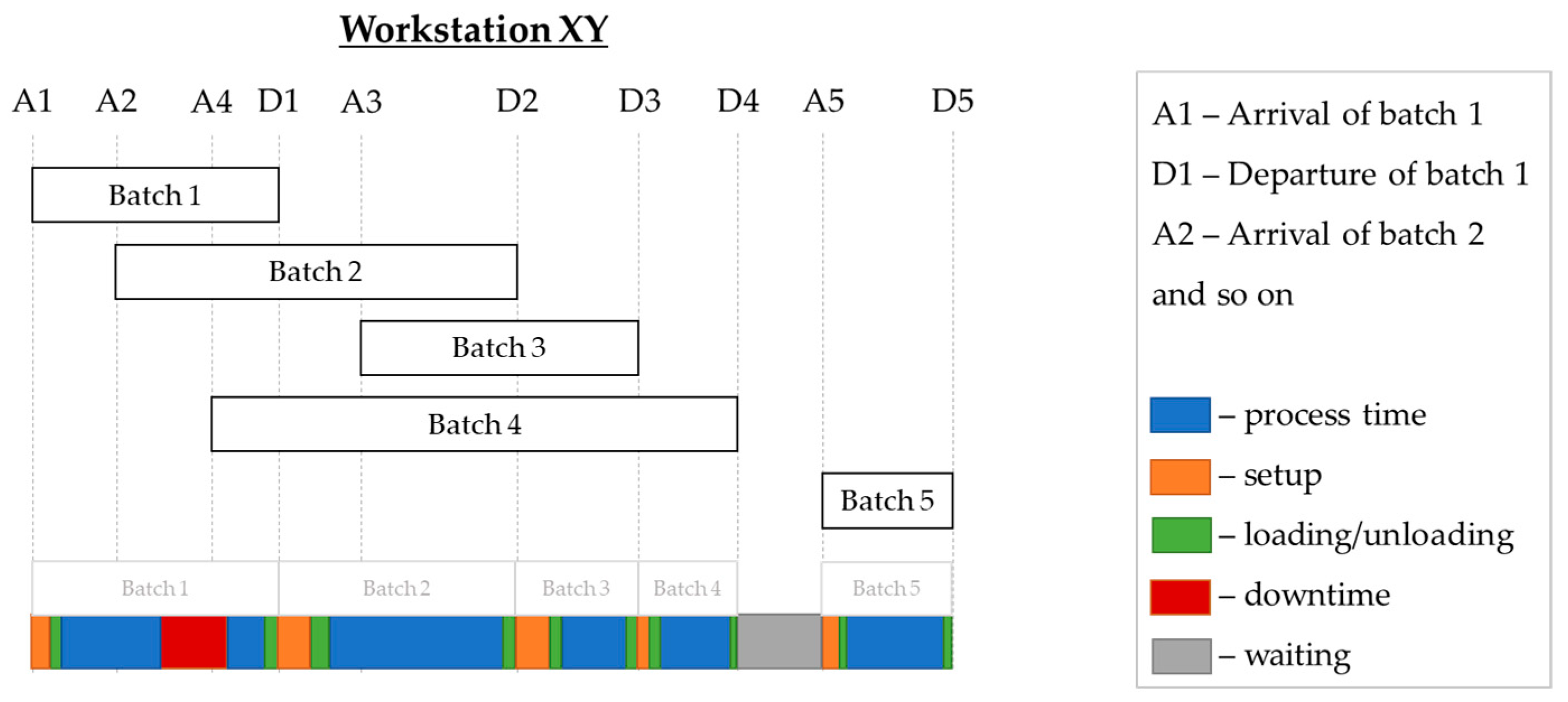
Jacobs, J. H. et al. present an approach to measure and quantify the temporal variability in semiconductor industry production systems using the effective process time [11]. They define effective process time as the time in which a batch claims the capacity of a production unit [11]. This means that the effective process time includes both the time at which a workstation is prepared to process a batch and the time at which the batch is effectively processed. The data required to calculate the effective process time are determined using an event-based approach. For this purpose, the authors acquire the arrival and departure events of the batches in the production unit (Figure 2) [12].

After a certain time, several effective process times are determined, resulting in a complete distribution of the effective process time. For the production unit, the average effective process time and the associated coefficient of variation can be calculated to investigate the inherent temporal variability. Extracting the raw process time from the effective process time shows the non-value-adding part. Setup times and/or downtimes of the production unit affect the effective process time. Consequently, the causes for inherent temporal variability can be limited to a certain extent. Hence, it must be questioned whether there are possibilities for a more detailed representation. In dividing variability into that which is controllable and uncontrollable, the approach offers no solution.

Lei, M. et al. describe a procedure for the determination of the overall equipment effectiveness (OEE) of machines/plants in the semiconductor industry [13]. In terms of inherent temporal variability, it is argued that the OEE can identify the causes of temporal variability via the deviations in performance, quality, or availability [14]. It should be noted that although indications can be given via the OEE, it is not possible to clearly narrow down the causes of temporal variability. It is also not possible to derive conclusions about the form of the variability. Besides that, the way Lei, M. et al. capture availability is interesting. For data acquisition to determine availability, they divide the production cycles into the production technical time components according to the SEMI E10 standard for the semiconductor industry. To determine a production technical time component, an event mapping module is used. The module assigns incoming events to a component of time according to defined rules and records them. Based on the data history, the availability is determined to calculate the OEE.

Eberts, D. et al. pursue in their publications the transformation of production systems in the semiconductor industry toward manufacturing with a continuous material flow. They describe the existing variability in production systems in this sector as the biggest challenge [15]. The combination of lean production and Six Sigma is intended to reduce the temporal and qualitative variability in the transformed production system [15]. Lean production methods and concepts are designed to empirically capture a variety of potential causes of variability. The multitude of recorded causes are analytically evaluated with the support of system experts using the methods and concepts of Six Sigma. The identified causes of variability are attempted to be eliminated. Variability that continues to exist is initially absorbed by buffers, which are then successively reduced within ‘Learning Loops’ [16]. ‘Learning Loops’ represent the concept of continuous improvement via lean production. The concept of Eberts et al. represents a comprehensive, methodical approach to the design of a material flow-based production system with a minimum of existing variability. The concept focuses on design elements to reduce the potential for variability rather than on an investigation of temporal variability to estimate the actual performance capability of the production system. Furthermore, the approach does not provide any information regarding the division of variability into that which is controllable and uncontrollable. Nevertheless, a data-based procedure to investigate temporal variability in production systems could support the concept and provide additional information.

In order to examine the extent to which inherent temporal variability is considered by the industry, production-related key performance indicators established on the shop floor are examined. The VDMA standard 66412-1 (from October 2009) lists 26 business and production-related key performance indicators for Manufacturing Execution Systems (MES), which are used to describe and evaluate the production systems [17,18]. The key performance indicators listed relate to productivity, the utilization of resources, or quality. Well-known quality indicators are included, such as the machine or process capability index, which considers qualitative variability. It is assumed that the key performance indicators have become established and are used in the industry. An indicator to investigate the inherent temporal variability in production systems is missing.

To summarize, the presented approaches are expandable and do not provide information about what causes the existing temporal variability or what forms of variability are present. The subdivision of variability is important to determine which causes can be influenced and which cannot. Influenceable causes can be eliminated or reduced. If they cannot be eliminated or reduced, they can be considered in production planning. Furthermore, if the existence of uncontrollable events is known, how this form of variability can be converted can be examined. Predictive maintenance (PM) serves as an example. By observing the functional behavior of hardware components, deviations from the setpoint can be detected in order to initiate planned maintenance work in advance. Instead of a random failure due to an unconscious fault that takes production by surprise and needs time to be found, a controllable maintenance event can be initiated. The value-adding availability of the workstation decreases, but the impact is less than if an event of true randomness occurs. Therefore, PM emphasizes that improving information can reduce randomness and thus unconscious events in a system, leading to an increase in productivity.

As was pointed out, inherent temporal variability in production systems influences production scheduling, the scheduling of deliveries, capacity planning or resource availability, inventory management, as well as cost development [19]. The improvement potentials identified in this paper relate to the fulfillment of production schedules based on complete data as well as to the increase in system performance. These are the research objectives. Complete data result from the inclusion of inherent temporal variability in the planning processes. Thus, the actual performance level of a production system can be determined to derive achievable planned values. An increase in system performance can be achieved by reducing the system’s inherent temporal variability.

After giving background information and describing the research objectives, the introduction provides an overview of previous research activities investigating inherent temporal variability. In the following, this paper addresses the development of a systematic approach to investigate the inherent temporal variability in production systems. The testing of the approach as well as the results are then summarized. Finally, the findings are discussed and concluded. It has to be mentioned that this research project focuses on discrete production systems with repetitive process steps, i.e., of any kind of manufacturing, with the exception of custom and one-off production. In addition, a production system with a certain degree of digitization is required in which data can be collected and processed. First, in order to consider inherent temporal variability in production planning, it must be measurable and quantifiable, which leads to the following research question: how can inherent temporal variability be measured, quantified, and included in production planning and control to improve it?

2. Development of a Systematic Approach to Investigate Temporal Variability

2.1. Preliminary Considerations

During the realization of a production schedule, several variables are observed. There are dependent variables, such as planned values or key performance indicators, which are measured. Furthermore, there are independent variables, which should influence production in favor of the dependent variables, such as lot or batch sizing, order release rules, etc. Finally, there are extraneous or disturbance variables, which cause unplanned temporal variability during production and are the subject of this research project due to their negative influence on the dependent variables. Extraneous or disturbance variables are unplanned events that provoke delays of planned operations or trigger unplanned operations. Some of them can be registered and are already known, e.g., machine breakdowns, and others only become apparent through the specific investigation.

Previous work on this topic has already used event-based approaches to capture temporal variability in production systems and to narrow down its causes. This will now be continued and extended via an automated procedure. In this context, digital events are captured from the shop floor to generate data from which operations that have occurred can be derived. Depending on the viewpoint, the operations can be assigned to the existing components of the lead time of the jobs or states of the workstation. This enables the causes of temporal variability to be narrowed down.

2.2. Automated and Event-Based Procedure for Generating the Required Data

The data base to which the approach is applied is created via an automated, event-driven procedure. Herein, the lead time components of the jobs and/or states of the production system are recorded based on digital events. To be able to record the digital events, a corresponding degree of digitization of production is essential. This can still be problematic for small and medium-sized enterprises at present due to the slow pace of digital transformation, but it should be increasingly possible in the future [20] (pp. 73–76).

The automated, event-driven procedure is realized via a software application consisting of four functional units:

• Event or data acquisition;
• Data persistence and pre-processing;
• Data processing and manipulation;
• Data analysis and evaluation.

In event or data acquisition, digital events are acquired from the shop floor. This means that the hardware components of the production objects and associated systems on the shop floor provide signal data in the form of digital events. Digital events indicate physical events. Physical events trigger operations, which in turn refer to lead time components and/or states. When capturing digital events, their uniqueness must be ensured. This means that a digital event may only refer to one operation in order to generate an error-free data base. If a digital event refers to several operations, event combinations are required for an unambiguous assignment. Uniqueness and correctness are only two of several data quality criteria that must be ensured. If higher-level systems such as an MES are available, the digital events or status data can be recorded via them. The functional units ‘event or data acquisition, data persistence and pre-processing, data processing and manipulation’ may then be omitted. When using higher-level software systems, the selection of lead time components and/or states can be limited or predefined via the system.

There are various options for data persistence depending on the type of data and their properties. If the data approach the characteristics of big data, NoSQL data bases, cloud systems, data warehouses, or data lakes are used. After the digital events have been acquired and persisted, they are pre-processed. This means that data from different sources must be converted into a consistent format.

If the format of the data is consistent for further processing, the defined lead time components and/or states are assigned based on the events or event combinations recorded. The respective durations of the individual events can then be calculated from the associated time stamps. The data can be taken from a higher-level system, and the occurrence and duration of the operations are usually available so that no further processing of the data is necessary. During the data processing, the data can be aggregated with other data, such as product type or material batch. In this way, more information can be generated, and analysis can be performed with contextual information. With data manipulation, erroneous data are cleansed or corrected if necessary.

The last functional unit is used for data analysis as well as for numerical and graphical evaluation. The software application is intended for industrial use and is also referred to as a data pipeline. Thus, the data pipeline is composed of several programs corresponding to the functional units. The functional units can form independent programs (open source or commercial variants) or be developed as stand-alone programs.

2.3. KPI-Driven and Data-Based Procedure to Investigate Temporal Variability

The potential causes of inherent temporal variability are narrowed down via the production-related time components of the lead time from the job viewpoint. From the viewpoint of the workstation, the respective states can also be used. In general, it is recommended to take both viewpoints in order to obtain as much (contextual) information as possible to identify the causes of inherent temporal variability. It should be noted that the subdivision of lead time as well as the states found in production systems may differ between systems. Figure 3 shows an example of the pursued procedure from the viewpoint of the workstation.

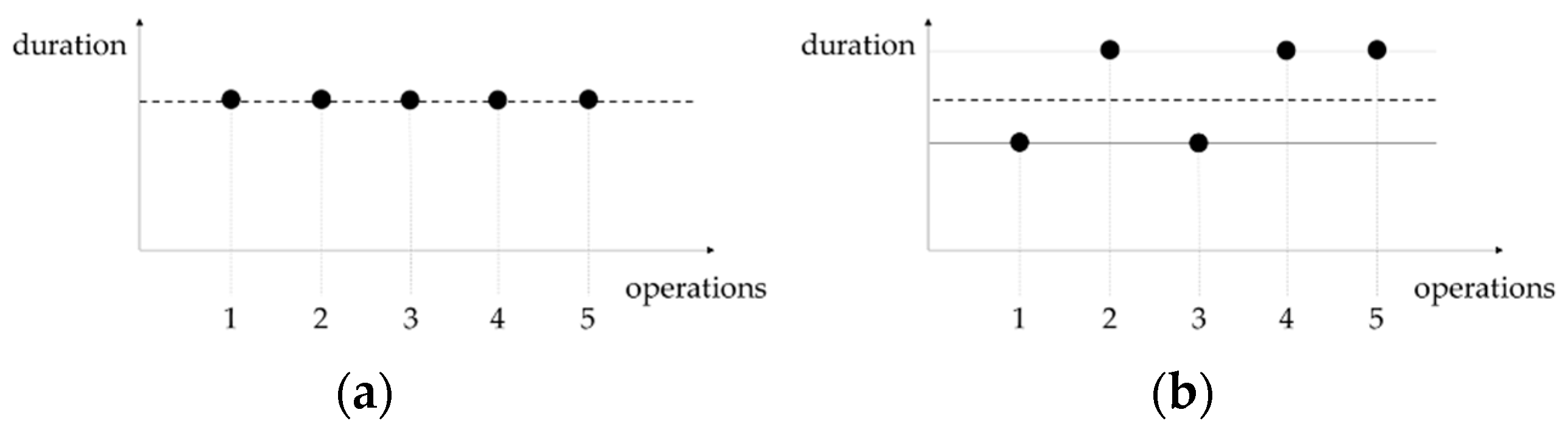
Every operation and thus every state the system can be in during the production time is recorded within a defined time period. This period can be a shift, a day, a week, and so on. Within the time period, the sum of states or, more precisely, the occurred operations per state are investigated for inherent temporal variability. For this purpose, a statistical parameter is modified. The parameter measures the deviations in the durations so that operations with the same or similar durations are investigated. Operations with the same duration follow a uniform planned value (Figure 4a), and operations with similar durations a determined target value (Figure 4b).

For that reason, this research project focuses on production systems with repetitive process steps. A planned, persistent irregularity in the duration of the operations as well as the deliberate combination of operations of different durations, which cause an increase in the corridor, impair the validity of the approach.

The statistical parameter that is modified to investigate inherent temporal variability was created by Erdlenbruch, B. He established the connection between the weighted mean, the arithmetic mean (average), and the variance [21] (pp. 31–35). The average lead time represents the average value of the number of jobs processed via the system during the period under consideration. The weighted mean lead time is a time-based average that considers the direct workload per job [21] (p. 31). For jobs with similar workloads, the average lead time is sufficient [21] (p. 31). If the workload of the jobs varies by a multiple, the weighted mean lead time should be used as a representative measure [21] (p. 31). For this purpose, Erdlenbruch, B. introduced the measure of relative variance to characterize variability [21] (p. 31). Using the measure of relative variance and the arithmetic mean, the weighted mean can be calculated, which can be demonstrated using an ideal production process. An ideal production process is characterized by the following conditions:

• At any time, there is exactly one job at each workstation (utilization = 100%);
• A job is processed immediately after its arrival at the workstation (lead time = theoretically best possible lead time) [22] (p. 68).

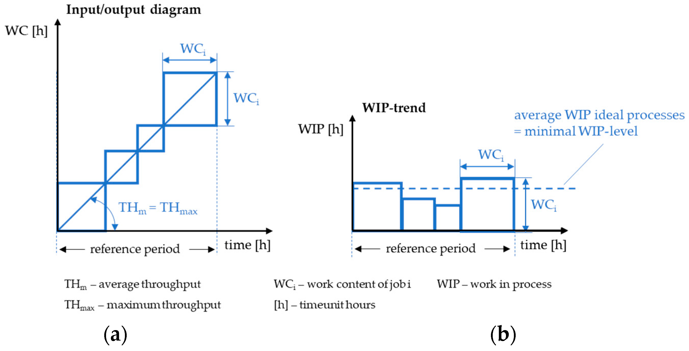
The input/output diagram of an ideal production process is shown in Figure 5, wherein the axes denote the time required for the workstation and the lead time [23] (p. 61).

Ideally, the time required for the workstation (planned time = planT) corresponds to the production time (actual time = actT). The minimum workload (work in process = WIPmin) can be calculated from the planned and actual values (n = number of values):

$${\mathrm{W}\mathrm{I}\mathrm{P}}_{\mathrm{m}\mathrm{i}\mathrm{n}}=\frac{\sum _{\mathrm{i}=1}^{\mathrm{n}}\left({\mathrm{p}\mathrm{l}\mathrm{a}\mathrm{n}\mathrm{T}}_{\mathrm{i}}\ast {\mathrm{a}\mathrm{c}\mathrm{t}\mathrm{T}}_{\mathrm{i}}\right)}{\sum _{\mathrm{i}=1}^{\mathrm{n}}{\mathrm{p}\mathrm{l}\mathrm{a}\mathrm{n}\mathrm{T}}_{\mathrm{i}}};\mathrm{i}\mathrm{f}\mathrm{a}\mathrm{c}\mathrm{t}\mathrm{T}=\mathrm{p}\mathrm{l}\mathrm{a}\mathrm{n}\mathrm{T},$$

(1)

where the actual values ideally correspond to the planned values [23] (p. 61):

$${\mathrm{W}\mathrm{I}\mathrm{P}}_{\mathrm{m}\mathrm{i}\mathrm{n}}=\frac{\sum _{\mathrm{i}=1}^{\mathrm{n}}\left({\mathrm{p}\mathrm{l}\mathrm{a}\mathrm{n}\mathrm{T}}_{\mathrm{i}}\ast {\mathrm{p}\mathrm{l}\mathrm{a}\mathrm{n}\mathrm{T}}_{\mathrm{i}}\right)}{\sum _{\mathrm{i}=1}^{\mathrm{n}}{\mathrm{p}\mathrm{l}\mathrm{a}\mathrm{n}\mathrm{T}}_{\mathrm{i}}}$$

(2)

In contrast with the ideal case (blue), reality (grey) is subject to variability, regardless of whether homogeneous or heterogeneous production conditions are present (Figure 6).

In this case, statistical quantities such as the arithmetic mean (M) (Equation (3)) and the variance (s²) (Equation (4)) are used to determine the actual inventory [23] (p. 62):

$${\mathrm{a}\mathrm{c}\mathrm{t}\mathrm{T}}_{\mathrm{M}}=\frac{\sum _{\mathrm{i}=1}^{\mathrm{n}}{\mathrm{a}\mathrm{c}\mathrm{t}\mathrm{T}}_{\mathrm{i}}}{\mathrm{n}},$$

(3)

$${\mathrm{a}\mathrm{c}\mathrm{t}\mathrm{T}}_{\mathrm{s}2}=\frac{\sum _{\mathrm{i}=1}^{\mathrm{n}}\left({\mathrm{a}\mathrm{c}\mathrm{t}\mathrm{T}}_{\mathrm{i}}\ast {\mathrm{a}\mathrm{c}\mathrm{t}\mathrm{T}}_{\mathrm{M}}\right)2}{\mathrm{n}}$$

(4)

Instead of n, (n − 1) is also written as a divisor since no variance can occur with a single observation but only with at least two observations. Since the sample sizes within this research project are assumed to be sufficiently large and all values are decisive, n is taken as the divisor. After solving the formula for calculating the variance (Equation (5)) and inserting other formulas, the relationship is obtained according to Equation (6):

$${\mathrm{a}\mathrm{c}\mathrm{t}\mathrm{T}}_{\mathrm{s}2}=\frac{\sum _{\mathrm{i}=1}^{\mathrm{n}}\left({\mathrm{a}\mathrm{c}\mathrm{t}\mathrm{T}}_{\mathrm{i}}^2-2{\ast \mathrm{a}\mathrm{c}\mathrm{t}\mathrm{T}}_{\mathrm{i}}\ast {\mathrm{a}\mathrm{c}\mathrm{t}\mathrm{T}}_{\mathrm{M}}+{\mathrm{a}\mathrm{c}\mathrm{t}\mathrm{T}}_{\mathrm{M}}^2\right)}{\mathrm{n}}$$

(5)

$$\frac{{\mathrm{a}\mathrm{c}\mathrm{t}\mathrm{T}}_{\mathrm{s}2}}{{\mathrm{a}\mathrm{c}\mathrm{t}\mathrm{T}}_{\mathrm{M}}}+{\mathrm{a}\mathrm{c}\mathrm{t}\mathrm{T}}_{\mathrm{M}}=\frac{\sum _{\mathrm{i}=1}^{\mathrm{n}}({\mathrm{a}\mathrm{c}\mathrm{t}\mathrm{T}}_{\mathrm{i}}\ast {\mathrm{a}\mathrm{c}\mathrm{t}\mathrm{T}}_{\mathrm{i}})}{\sum _{\mathrm{i}=1}^{\mathrm{n}}{\mathrm{a}\mathrm{c}\mathrm{t}\mathrm{T}}_{\mathrm{i}}}$$

(6)

In a real production system, the time (actual time) required to process the production schedule (planned time) varies. This results in Equation (7):

$$\frac{{\mathrm{a}\mathrm{c}\mathrm{t}\mathrm{T}}_{\mathrm{s}2}}{{\mathrm{a}\mathrm{c}\mathrm{t}\mathrm{T}}_{\mathrm{M}}}+{\mathrm{a}\mathrm{c}\mathrm{t}\mathrm{T}}_{\mathrm{M}}=\frac{\sum _{\mathrm{i}=1}^{\mathrm{n}}({\mathrm{p}\mathrm{l}\mathrm{a}\mathrm{n}\mathrm{T}}_{\mathrm{i}}\ast {\mathrm{a}\mathrm{c}\mathrm{t}\mathrm{T}}_{\mathrm{i}})}{\sum _{\mathrm{i}=1}^{\mathrm{n}}{\mathrm{p}\mathrm{l}\mathrm{a}\mathrm{n}\mathrm{T}}_{\mathrm{i}}}$$

(7)

As a result, the actual workload can be calculated using the weighted mean (wM):

$${\mathrm{W}\mathrm{I}\mathrm{P}}_{\mathrm{a}\mathrm{c}\mathrm{t}}={\mathrm{a}\mathrm{c}\mathrm{t}\mathrm{T}}_{\mathrm{M}}+\frac{{\mathrm{a}\mathrm{c}\mathrm{t}\mathrm{T}}_{\mathrm{s}2}}{{\mathrm{a}\mathrm{c}\mathrm{t}\mathrm{T}}_{\mathrm{M}}}=\frac{\sum _{\mathrm{i}=1}^{\mathrm{n}}\left({\mathrm{p}\mathrm{l}\mathrm{a}\mathrm{n}\mathrm{T}}_{\mathrm{i}}\ast {\mathrm{a}\mathrm{c}\mathrm{t}\mathrm{T}}_{\mathrm{i}}\right)}{\sum _{\mathrm{i}=1}^{\mathrm{n}}{\mathrm{p}\mathrm{l}\mathrm{a}\mathrm{n}\mathrm{T}}_{\mathrm{i}}}$$

(8)

Therefore, the actual workload in time units is equal to the weighted mean of the lead time according to Equation (9):

$${\mathrm{a}\mathrm{c}\mathrm{t}\mathrm{T}}_{\mathrm{w}\mathrm{M}}={\mathrm{a}\mathrm{c}\mathrm{t}\mathrm{T}}_{\mathrm{M}}+\frac{{\mathrm{a}\mathrm{c}\mathrm{t}\mathrm{T}}_{\mathrm{s}2}}{{\mathrm{a}\mathrm{c}\mathrm{t}\mathrm{T}}_{\mathrm{M}}}$$

(9)

Taking the coefficient of variation (CoV), the measure of relative variance (highlighted in bold) is obtained using Equation (10):

$${\mathrm{a}\mathrm{c}\mathrm{t}\mathrm{T}}_{\mathrm{w}\mathrm{M}}={\mathrm{a}\mathrm{c}\mathrm{t}\mathrm{T}}_{\mathrm{M}}\ast (\mathbf{1}+{\mathbf{a}\mathbf{c}\mathbf{t}\mathbf{T}}_{\mathbf{C}\mathbf{o}\mathbf{V}}^2)$$

(10)

Thus, the connection between the weighted mean, the arithmetic mean, and the variance or the measure of relative variance is clarified. If there are no fluctuations and the actual time corresponds to the planned time, the arithmetic mean value equates to the weighted mean value (Equation (13)):

$$\frac{{\mathrm{a}\mathrm{c}\mathrm{t}\mathrm{T}}_{\mathrm{s}2}}{{\mathrm{a}\mathrm{c}\mathrm{t}\mathrm{T}}_{\mathrm{M}}}+{\mathrm{a}\mathrm{c}\mathrm{t}\mathrm{T}}_{\mathrm{M}}=\frac{\sum _{\mathrm{i}=1}^{\mathrm{n}}({\mathrm{p}\mathrm{l}\mathrm{a}\mathrm{n}\mathrm{T}}_{\mathrm{i}}\ast {\mathrm{p}\mathrm{l}\mathrm{a}\mathrm{n}\mathrm{T}}_{\mathrm{i}})}{\sum _{\mathrm{i}=1}^{\mathrm{n}}{\mathrm{p}\mathrm{l}\mathrm{a}\mathrm{n}\mathrm{T}}_{\mathrm{i}}},$$

(11)

$${\mathrm{a}\mathrm{c}\mathrm{t}\mathrm{T}}_{\mathrm{M}}=\frac{\sum _{\mathrm{i}=1}^{\mathrm{n}}({\mathrm{p}\mathrm{l}\mathrm{a}\mathrm{n}\mathrm{T}}_{\mathrm{i}}\ast {\mathrm{p}\mathrm{l}\mathrm{a}\mathrm{n}\mathrm{T}}_{\mathrm{i}})}{\sum _{\mathrm{i}=1}^{\mathrm{n}}{\mathrm{p}\mathrm{l}\mathrm{a}\mathrm{n}\mathrm{T}}_{\mathrm{i}}},$$

(12)

$${\mathrm{a}\mathrm{c}\mathrm{t}\mathrm{T}}_{\mathrm{M}}={\mathrm{p}\mathrm{l}\mathrm{a}\mathrm{n}\mathrm{T}}_{\mathrm{w}\mathrm{M}}$$

(13)

In this case, the measure of relative variance is one because the variance is zero. It should be clarified that a value equal to one stands for ideal plannability, wherein the arithmetic value corresponds to the weighted mean. An ideal planning value does not mean that there is no temporal variability but instead states that the inherent temporal variability has been optimally integrated into the production planning and is predictable.

Erdlenbruch, B. investigated the lead time behavior of highly manual workstations to develop new job management procedures. Thereby, he focused on the execution time, which consisted of the setup time and the processing time. The reason for concentrating on the execution time was the continuous existence of jobs and the associated waiting times. The findings from his work are adopted herein. Time delays of operations are captured using the measure of relative variance to calculate the weighted mean. During modification, the term ‘variability level’ is introduced synonymously for the measure of relative variance.

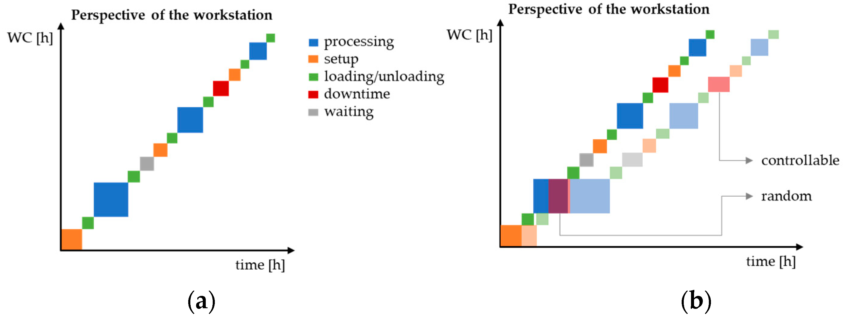
The variability level is measured for each lead time component and/or state. A workstation serves as an example. From the viewpoint of the workstation, the following states,

• Processing;
• Setup;
• Waiting;
• Loading/unloading;
• Downtime,

occur during the runtime of the station. Waiting at the station is intended, for example, due to different processing times at previous production units, intermediate processes (drying or curing processes), transport processes, or operations for lot/batch size optimization. Downtimes are planned maintenance intervals. Ideally, according to the production schedule, the operations per state correspond to those according to Figure 7a.

With regard to the occurring states, Figure 7b is not an ideal case in the sense of an ideal production process, since value-destroying components, such as waiting, are present. The idea of the ideal case shown herein is based on the assumption that the actual values correspond to the planned values with regard to the quantity and duration of the operations per state. In reality, there are deviations that affect the actual production time (actual time). Figure 7b contains inherent temporal variability, whereby the duration of the operations per state increases unplanned. The figure shows a random event in the form of an unplanned interruption during the first processing. Planned maintenance is also affected by fluctuations, but in contrast with unplanned downtime, this is a planned, controllable intervention that has been delayed unplanned. Since each operation per state can be affected by temporal variability at any time, each state must also be examined, as shown in the modified equation (Equation (14)). The variable t represents the affected lead time component or state that is examined:

$${\mathrm{t}}_{\mathrm{w}\mathrm{M}}={\mathrm{t}}_{\mathrm{M}}+\frac{{\mathrm{t}2}_{\mathrm{S}}}{{\mathrm{t}}_{\mathrm{M}}}={\mathrm{t}}_{\mathrm{M}}\ast (1+{\mathrm{t}2}_{\mathrm{C}\mathrm{o}\mathrm{V}})$$

(14)

Once the data are acquired for a given time period, the lead time components and/or states are investigated for inherent temporal variability via the variability level.

Inherent temporal variability can occur as time delays in planned operations or unplanned operations. Unplanned operations may occur in the time frame of the planned operations that cannot be detected with the variability level. Therefore, the number of operations of lead time components and/or states must also be considered and compared with the planned quantity. Therefore, at least two metrics are required.

In addition to the KPI-driven measurement and quantification of the existing temporal variability, it is also necessary to analyze what form of variability is present. This is conducted in two ways. First, the recorded quantity of operations is compared with the planned operations per lead time component and/or state to determine the number of unplanned operations. The second way uses the durations of the operations. It is assumed that events causing uncontrollable variability surprise production with their unconscious occurrence and lead to significant time delays in operations. For this reason, it is hypothesized that uncontrollable variability—in addition to the number of unplanned operations—can be determined by identifying outlier values. To define outlier values, the structure of boxplots is used. [24] Accordingly, outliers in this research project form values that

• Are below the difference between the 25% quartile and 1.5 times the interquartile range (IQR) of the state;
• Are above the sum of the 75% quartile and 1.5 times the IQR of the state.

A further subdivision according to the type of randomness is conceivable, considering the extreme outliers (three times the IQR), but cannot be said at this stage.

2.4. Consideration of the Investigated Temporal Variability in Production Planning and Control

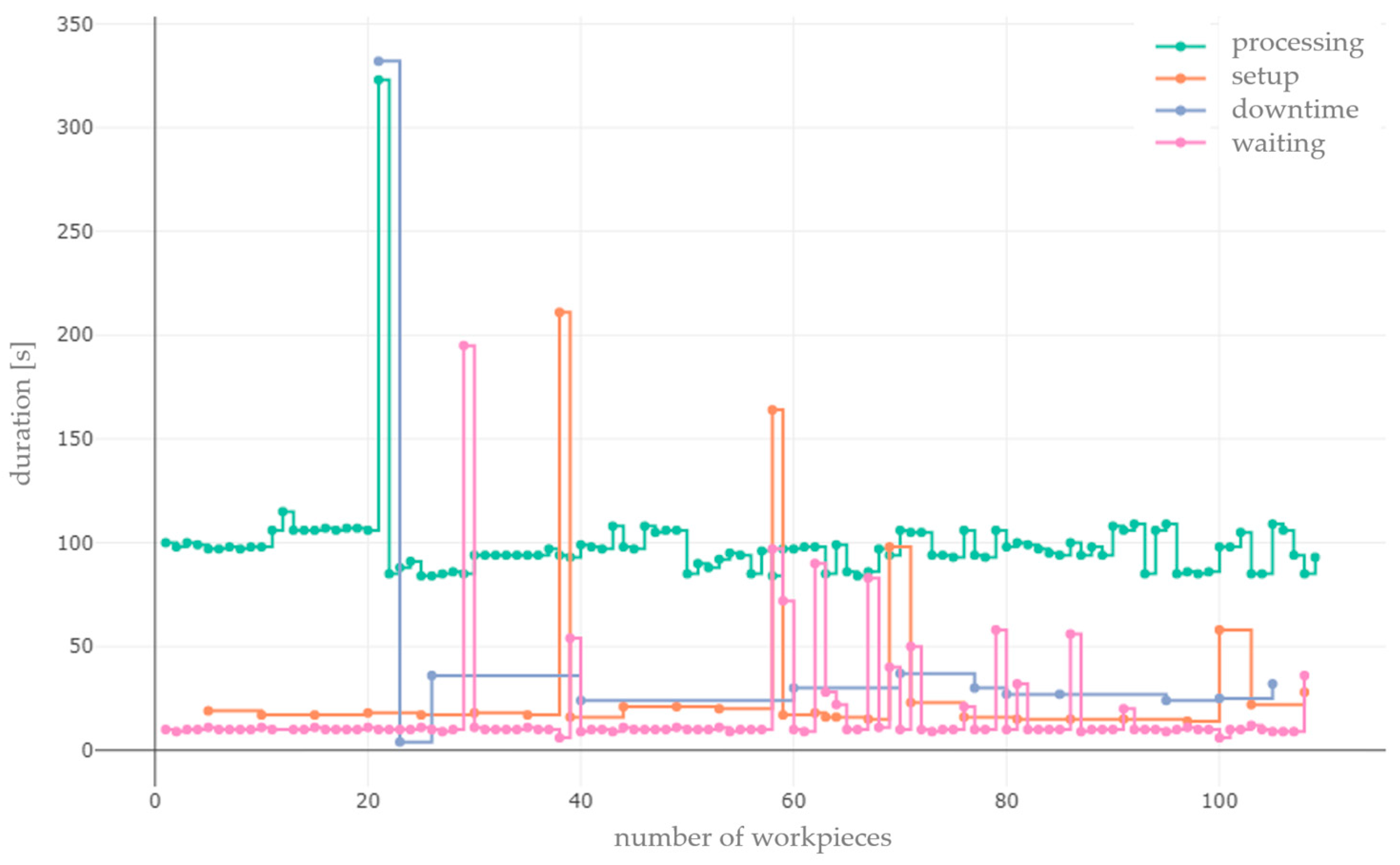
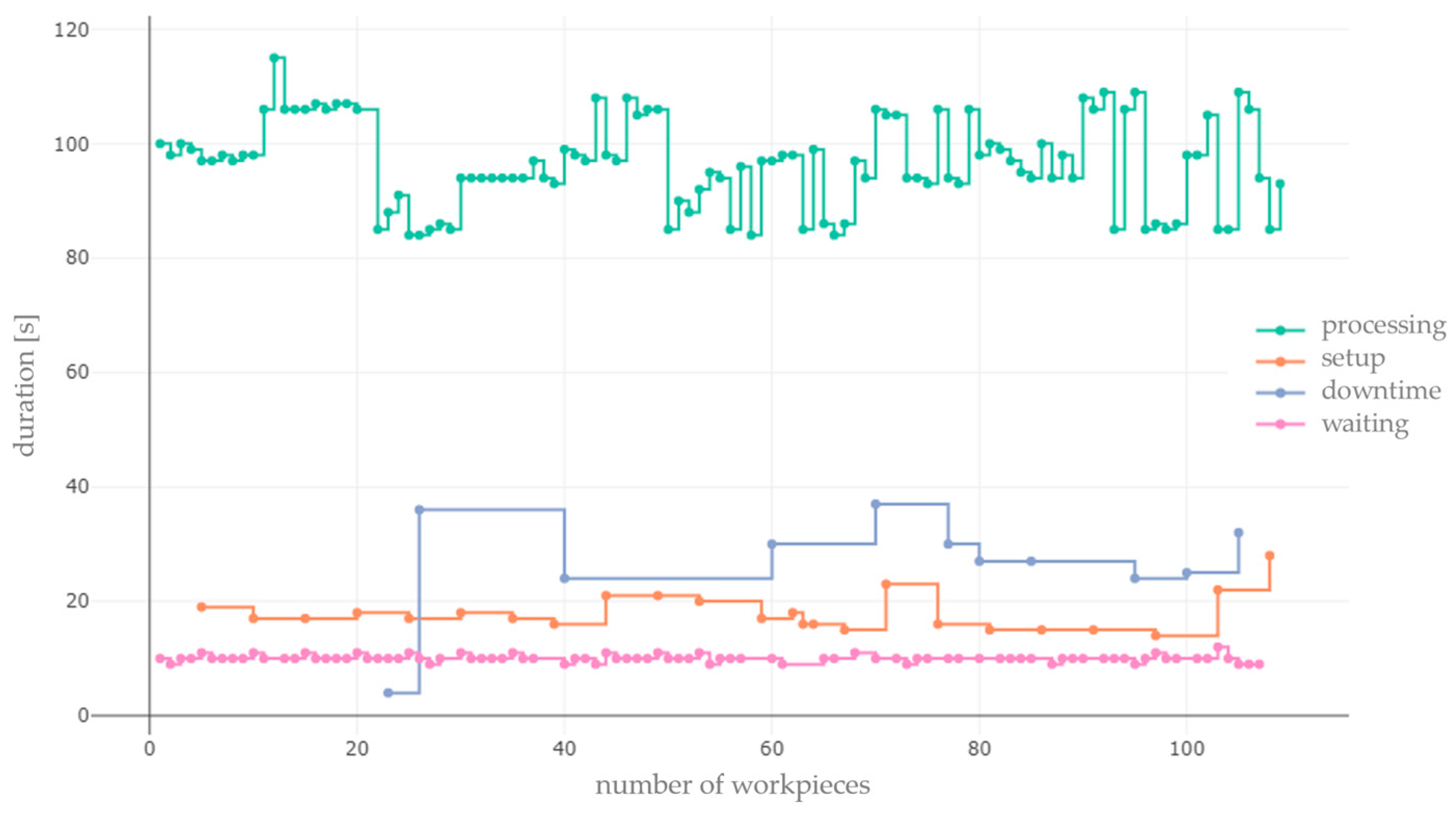
Once the inherent temporal variability per lead time component and/or state has been captured, measured, and quantified, and the form of the variability in the system has been derived, the operations or events that cause it need to be identified. This can be carried out by using time series plots for each lead time component and/or state (Figure 8).

The x-axis shows the number of workpieces, whereby the processing state serves as a reference. A mark on the line represents an operation. For the other states, this means that an operation has occurred after a corresponding number of workpieces have been produced. Several workpieces belong to one job.

For more precise identification, further subdivisions can be made, e.g., by product type or job. In the case of further subdivisions, however, the representativeness of the data in terms of data quantity and quality must be ensured. The y-axis contains the associated durations of the operations. Within a time series, the influence of known disturbance variables can be detected via causal relationships, and their influence can be evaluated based on the frequency and intensity of occurrence. Irregularities can also be detected and assigned to the operations or events that disrupt production. The events may be known or unknown, which also depends on the amount of uncontrollable variability in the system.

The combination of the numerical and graphical examination allows conclusions to be made as to whether the disturbance variables are known or unknown and whether they can be influenced or not. Furthermore, the necessary need for action can be derived depending on the influence on the production system in order to decide which causes are to be eliminated first. If required, it can be determined whether the provision of further data or information is possible in order to convert one form of variability into another. Actions against temporal variability in production systems can only be implemented if the causative events are known and influenceable. Action can also be taken by considering the events in the planning processes if avoidance is not possible. Consequently, the occurrence of ‘conscious and not influenceable’ events is not conceivable.

To include the existing temporal variability in the planning process, the weighted mean, which contains the variability level, is used. Critically, taking inherent temporal system variability into account is the equivalent of holding temporal buffers. The difference with common approaches is that the temporal buffers are determined based on data (instead of intuitively). Adjustments are carried out iteratively over the defined periods.

For future production cycles, the weighted mean of the lead time components and/or states is used in combination with the expected number of operations to calculate the required lead time. However, the approach needs to be revised. The consideration of the determined temporal variability in the captured scope is not representative of future planning cycles, because the outliers influence the values too much. The complete inclusion of outlier values is critical, as these do not represent the real process. Most extreme outliers represent exceptional scenarios that should be avoided. It is necessary to consider the temporal variability in the system, which is composed of events that follow regularity. As such, it is irrelevant whether they cause controllable or uncontrollable variability. For the selection of representative data, which are then incorporated into the production planning, the boxplot structure is used again. The data base is cleansed of extreme outliers, which are assumed to represent actual exceptional scenarios in the production process. This is intended to generate a representative data base for forecasting future production cycles. The extreme outliers are then declared as values, which

• Are below the difference between the 25% quartile and three times the IQR of the state;
• Are above the sum of the 75% quartile and three times the IQR of the state.

After data cleansing, it must be ensured that the data are representative. When removing extreme outliers, it must be guaranteed that they really are outliers. It is also important to be aware that removing data can lead to loss of information.

After each cycle of observation, the aim is to realize improvement actions via the manipulation of independent variables. Consequently, the production conditions are constantly changing. Hence, the data of the time periods must be considered separately in the iterative application of this approach.

3. Case Study and Results

3.1. Case Study

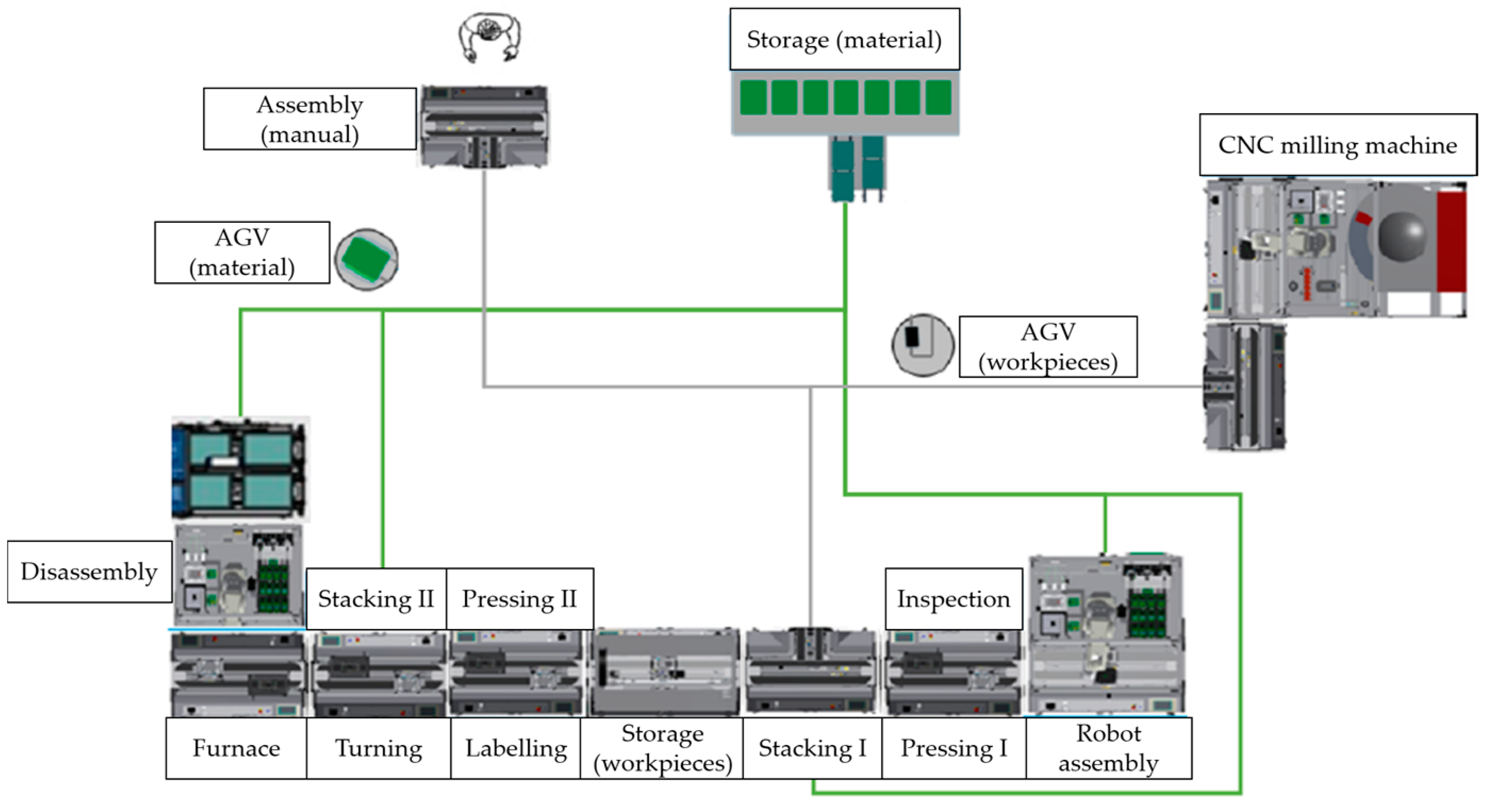
To test the systematic approach, the Industrial Internet of Things Test Bed (IIoT TB) of the University of Applied Sciences Dresden is used. The IIoT TB is a laboratory environment representing an automated production system of discrete manufacturing [25]. The IIoT TB has several processing stations, such as joining processes, thermal processes, assembly processes, inspection processes, etc., as can be seen in Figure 9.

The workpieces run automatically to the workstations via counter-rotating conveyor belts. Workstations separated from the main production line are supplied via autonomous guided vehicles (AGVs). Material is supplied manually and automatically via AGVs. Production is coordinated with the connected MES.

Initial testing in the laboratory means that there is no intervention in a real production environment, so there is no risk of interfering with actual production processes. In contrast, the complexity of the IIoT TB is limited or can be regulated compared with a real production system. Unlike a real system in the industry, the laboratory environment neither pursues business interests nor acts in a market-driven manner, which reduces the influence of external disruptive factors. In addition, the IIoT TB is a closed environment without influences from suppliers, adjacent departments, or customers.

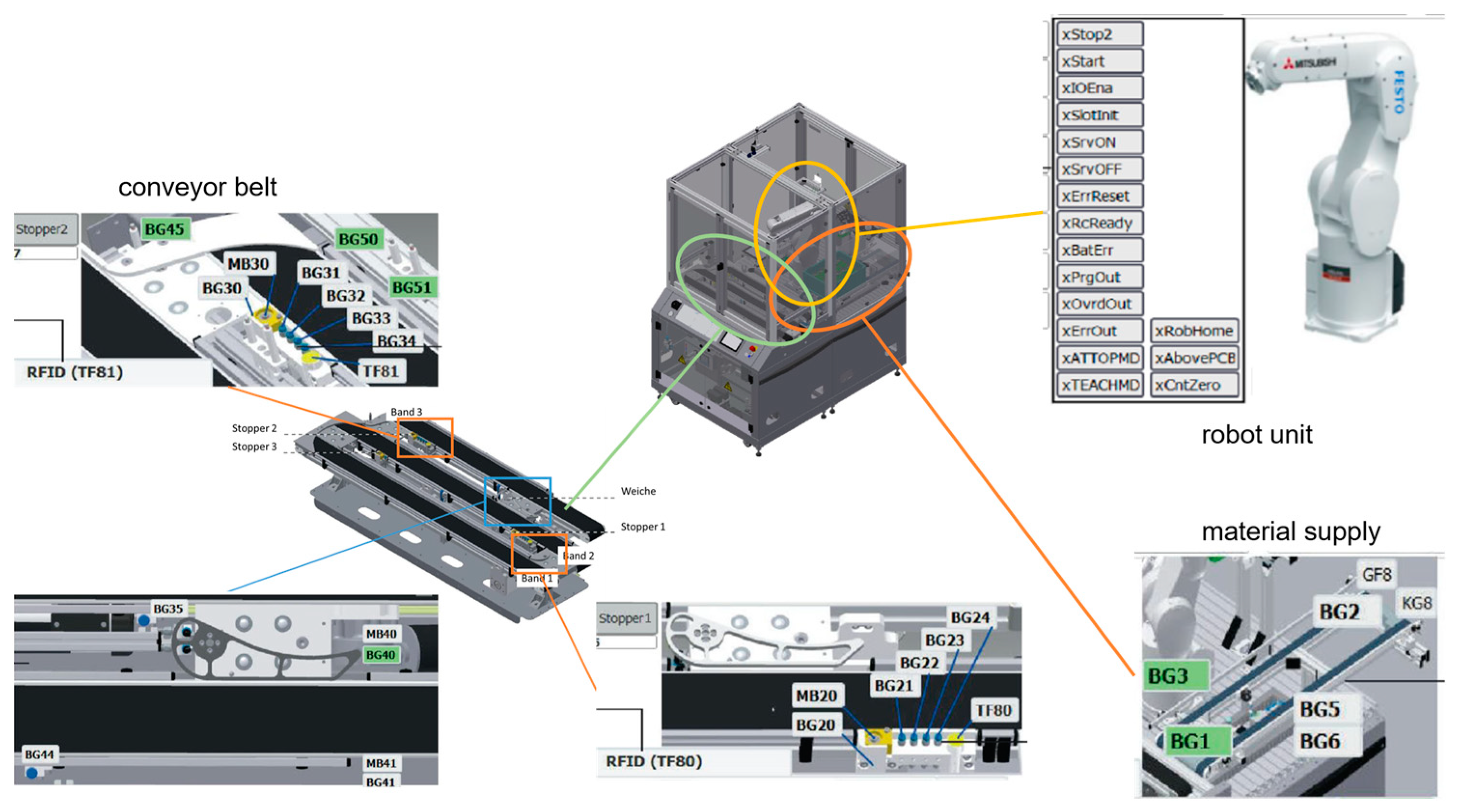
For the production system under consideration, the testing is limited to a single workstation of the IIoT TB to reduce the complexity. The workstation under investigation is a robot assembly cell, which is a bottleneck station of the overall system. In the robot assembly cell, a printed circuit board is placed into a plastic case employing a six-axis industrial robot and provided with up to two fuses (Figure 10). Via a conveyor belt, the workpieces enter the workstation fully automatically. The material setup of the robot assembly cell is partly manual, and for the testing of the approach, the material setup is just manual.

Due to limited functions and missing access points, the data of the integrated MES of the IIoT TB cannot be used. Instead, the digital events of the PLC of the robot assembly cell are acquired to subdivide the states of the workstation, as shown in Figure 10. The majority of the signal sources can be accessed via the PLC. Since there are no interfaces for accessing other hardware components, only digital events from the viewpoint of the workstation are recorded.

For the robot assembly cell, operations for the listed states can be recorded using the signal sources of the PLC:

• Processing;
• Setup;
• Waiting;
• Downtime.

Because of the limited signal sources, event combinations have to be created in some cases to be able to clearly assign operations to the corresponding states. For event combinations, a reference event has to be declared for the event or data acquisition, from which the output data (time stamp, etc.) are persisted for later data processing.

3.2. Experimental Design

For the testing, a production scenario is simulated that is similar to series production in terms of the number of product types and the structure of the production schedule. A production schedule consisting of several jobs is processed during an observation period of four hours. Four hours correspond to half a shift and form a test series. There are up to four test series. Normally, a job consists of ten workpieces. There are up to four different product types. The first four jobs consist of ten uniform types, and the other jobs consist of ten mixed types. During the observation period, the defined states are investigated for inherent temporal variability.

The design of the experimental environment is based on the contents of [26]. When setting up the experimental environment, dependent, independent, and extraneous variables are defined. The dependent variables are influenced by the independent and extraneous variables. The independent variables are intentionally manipulated, and the extent of manipulation is measured with the dependent variables. The extraneous variables represent uncontrollable confounding variables that may affect the results of the experiment.

For the testing of the systematic approach, the dependent variables are the planned and target values of production. While the deviations between the planned and actual values are minimized, the target values (KPIs) are continuously improved during the experiment. The planning procedure according to the developed approach is also compared with other approaches.

The independent variables form the design elements of the test setting and procedure. Thus, the workstation is completely set up at the beginning of the testing. The boxes of printed circuit boards each contain five boards of one type. The workstation can hold one box at a time. The containers for the glass fuses are filled with up to 45 glass fuses. There is no job release rule. Subsequent jobs are released if the separate conveyor belt of the bottleneck station has free capacity. The separate conveyor belt of the station can take up to three workpieces on carriers. There are always ten carriers on the conveyor belt of the production system, which move to the workstations with or without workpieces. Downtimes are provoked at regular intervals via a dice mechanism (to simulate randomness). A dice is rolled once every five workpieces, a planned setup cycle of the printed circuit boards. If a double or a seven is rolled, the safety door is opened (as a simulation of a malfunction) and is not closed again until another double or a seven is rolled.

The manipulation of the independent variables is carried out between the test series. After each test series, the systematic approach is applied. The application is intended to identify potentials for improvement. The identified improvements are implemented successively in the form of the manipulation of independent variables.

Since the laboratory environment cannot be completely cleared of confounding variables, extraneous variables can influence the results. Extraneous variables or disruptive events can be caused by congestion on the conveyor belt of the production system, overtaking product types on the conveyor belt, or connection disturbances to the MES. These influences encourage the testing of the systematic approach since temporal variability in production systems is to be investigated. While the manipulation of the independent variables produces predictable variability, the extraneous variables provoke the occurrence of unplanned events, which must be captured and minimized.

The analysis of a test series ends with the measurement of the dependent variables. For the dependent variables, the following key performance indicators established in the industry are used as target values and compared within the test series:

• Overall equipment effectiveness (OEE);
• Productivity;
• Utilization factor (UF).

The OEE is the product of availability, performance, and quality. Availability is calculated by dividing the sum of the total process and waiting time by the available time (time without random downtime). For performance, the sum of good and reject parts is divided by the maximum throughput, while quality can be calculated by dividing the number of good parts by the sum of good and reject parts. Productivity is calculated via the division of good parts with maximal throughput. The UF is the ratio of the processing time to the total runtime.

Another key performance indicator is the throughput, which is initially determined as a planned value. At the beginning of the experiment, the planned throughput is calculated from the ideal lead times of the previously measured product types and the available capacity of the bottleneck station.

When determining the planned throughput for future production cycles, another alternative procedure is introduced in addition to the presented procedure to compare different planning approaches. The procedure originates from sales planning for forecasting future demand and is called first-order exponential smoothing. Since no examples of intuitive procedures can be found in the literature, the two stochastic approaches are compared with each other after each test series. This is intended to evaluate the reliability and practicability of the developed approach.

The developed approach uses the weighted mean and the number of operations per lead time component and/or state to determine the actual required capacity of the workstation. The figures are used to calculate future planned values. In contrast, the first-order exponential smoothing procedure calculates future planned values (planV_t+1) using the planned value determined in the previous period (planV_t), the actual value of the period (actV_t), and a smoothing factor (α) (Equation (15)) [27] (p. 78).

$${\mathrm{p}\mathrm{l}\mathrm{a}\mathrm{n}\mathrm{V}}_{\mathrm{t}+1}={\mathrm{p}\mathrm{l}\mathrm{a}\mathrm{n}\mathrm{V}}_{\mathrm{t}}+\mathsf{\alpha }\ast ({\mathrm{a}\mathrm{c}\mathrm{t}\mathrm{V}}_{\mathrm{t}}-{\mathrm{p}\mathrm{l}\mathrm{a}\mathrm{n}\mathrm{V}}_{\mathrm{t}})$$

(15)

The smoothing factor corresponds to a value between zero and one. The higher the smoothing factor, the more the immediate past is taken into account [27] (pp. 79–80). This means a high smoothing factor is recommended for short-term planning forecasts, and a low one for long-term ones. The literature recommends a value between 0.1 and 0.3 [27] (p. 80).

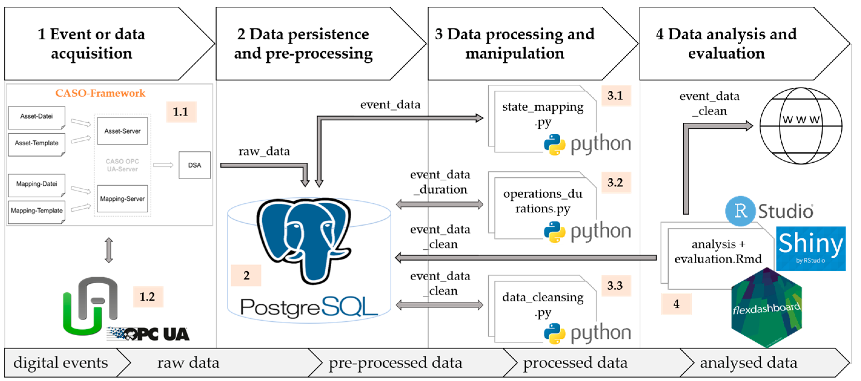
3.3. Data Pipeline of the Case Study

A data pipeline is created individually depending on the production system to be investigated. When selecting the programs to build the data pipeline, both existing open-source programs and programs created independently via open-source development environments are used. The free programming languages Python and R are used to create application-specific programs for the functional units. Figure 11 shows the structure of the data pipeline. The working and data sequence is indicated with the colored subitems.

For event or data acquisition, parts of the CASO framework are used to connect to the hardware components of the PLC (1.1). CASO (Capabilities-Based and Self-Organizing Manufacturing Management) has been a research project of two former colleagues of the author of the working group ‘Smart Production Systems’. Among other things, CASO provides a standardized data acquisition layer that supports OPC UA as a communication protocol. Digital events are acquired via the OPC UA communication standard [28,29,30]. For the selection of required signal sources, the graphical user interface of UA Expert is used (1.2).

To persist the events, the relational data base system of PostgreSQL is chosen due to the low data volume (2). As the data come from a single hardware component (the PLC), no pre-processing of the data is required.

Data processing, data manipulation, data analysis, and data evaluation are implemented via self-created programs. The programs access the data from the PostgreSQL data base and finish their run by creating a revised data set. The programs for data processing and manipulation are created via Python. During data processing, the operations resulting from the events or event combinations are assigned to the defined states (3.1). The calculation of the individual operation durations is performed using another Python program (3.2). A third program is used for data cleansing and belongs to data manipulation (3.3). This program prioritizes states if several events have occurred at the same time. For example, digital events of different signal sources that relate to a setup and waiting operation can be sent simultaneously. Since the workstation can only be in one state at a time, the setup state in this case would be prioritized until it is finished. It should be mentioned that only start events are declared for the test series. This means that a start event of a subsequent operation is also the end event of the previous operation. Therefore, data cleansing is required in some cases.

Data analysis and evaluation use cleansed data as the basis for numerical and graphical result presentation. This is realized using a web-based, interactive dashboard, which is created independently via the R programming language. The R packages Shiny and Rflexdashboard are used for this purpose (4).

3.4. Testing of the Systematic Approach

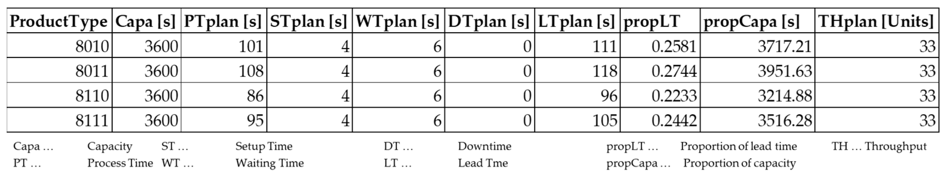
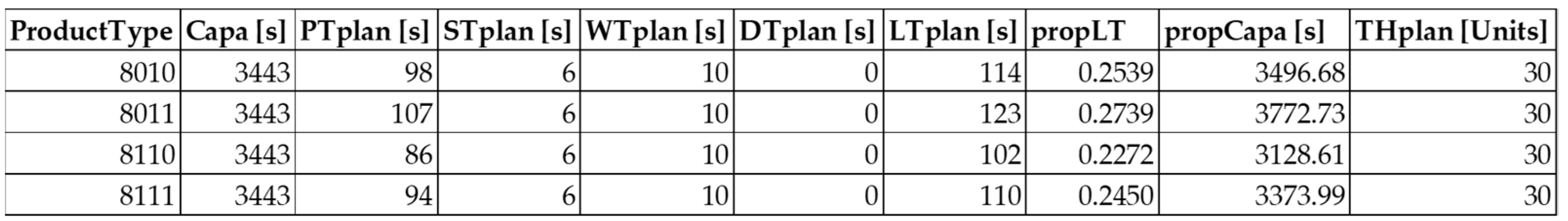
After the data pipeline has been built and validated, the test series for testing the systematic approach are carried out. The starting point for creating the production schedule is the data shown in Figure 12.

The data are based on an optimal production run of the workstation and represent the ideal case. Within 4 hours, the robot assembly cell manufactures a total of 132 workpieces.

For the test series, the planned values are first determined. After that, the independent variables are manipulated. Then, the test series are carried out, and the data base is generated via the data pipeline. The systematic approach is applied to the data base of each test series. Lastly, the target values are measured (and calculated) and compared with the previous values. In addition, the actual values are compared with the planned values.

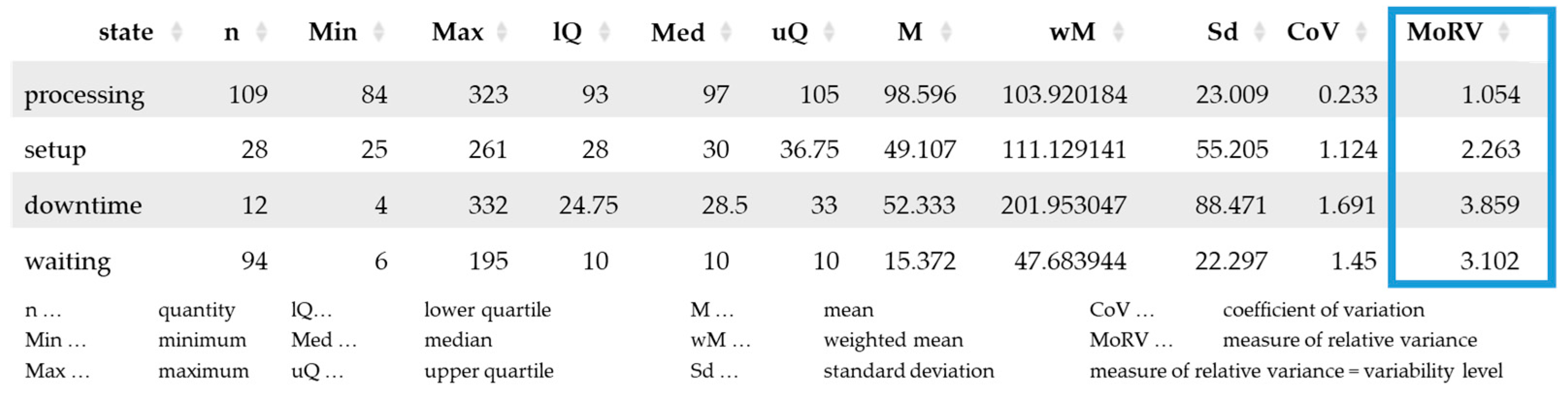
Figure 13 shows an example in which it can be seen that all the defined states are subject to inherent temporal variability.

First, we investigate which state is affected by temporal variability (via the variability level and quantity of operations) and whether it is controllable or uncontrollable variability. Unlike the other states in Figure 13, the processing state from test series one consciously contains variability (controllable variability) due to the grouping of the different product types. For this reason, the processing state has a relatively low variability level close to the optimal value of ‘1’.

In addition to numerical evaluation, graphical elements such as time series diagrams are also used to investigate disturbance variables. From the time series plots, causal relationships between the caused temporal variability and its confounding factors can be derived, if necessary. It can be observed that temporal variability within the states that are set up and waiting is caused by a lack of staff, poor organization during setup, faulty setup, and delayed job releases. The downtime is affected by random events. Subsequently, actions are determined to reduce, eliminate, or further influence the disruptive factors. A further influence can be the inclusion of the planning if a reduction or elimination is not possible.

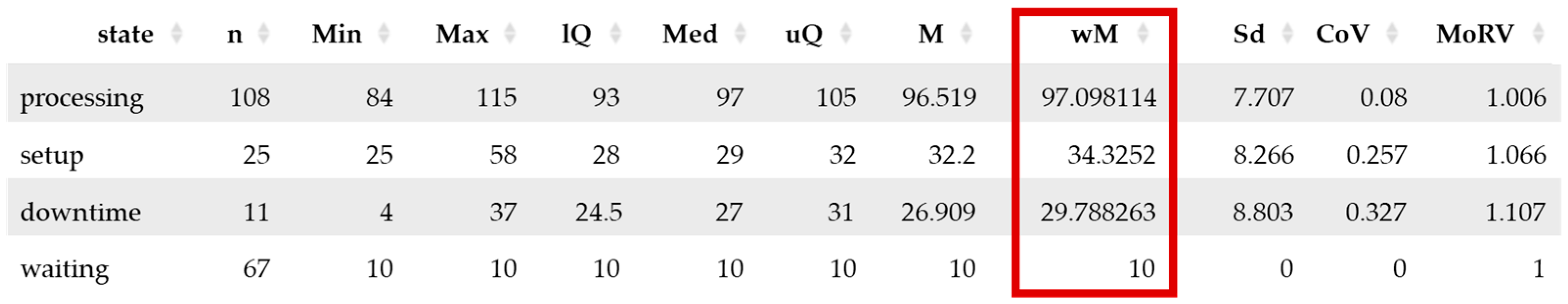
To incorporate the existing temporal variability into the planning process, the weighted mean per state derived from the data adjusted for extreme outliers is used. (Figure 14).

The differences between the data sets with and without adjustment for extreme outlier values can also be seen in a comparison of the time series plots in Figure 8 and Figure 15.

In addition to the weighted mean per state derived from the data adjusted for extreme outliers, the number of operations in which a regularity can be detected is included in the determination of the planned values for future production cycles. For the second test series, the application of the systematic approach results in the data in Figure 16 for production scheduling.

In summary, to determine the future planned throughput via the systematic approach, the maximum capacity of the production system is reduced with random downtime. The resulting available capacity is then used to create the production schedule. For this purpose, the weighted mean and the number of operations are incorporated to derive the planned throughput for the future production cycle.

Before conducting test series two, the independent variables are manipulated by implementing improvement actions. Scheduled maintenance is introduced and performed after 20 processed workpieces for 30 s per operation (affecting the downtime). A simulated malfunction is replaced for this purpose. This also reduces the probability of a fault event occurring. The safety door is now only opened when a double is rolled and is closed again with a double or a seven. The boxes with the printed circuit boards are prepared with uniform and mixed types (affecting the setup). An improvement action related to waiting is implemented by introducing an appropriate job release rule.

Due to the change in the experimental conditions resulting from the introduction of scheduled maintenance, the data used to create the production schedule for the second test series must be adjusted (Figure 17).

Regarding the manipulation of the independent variables, before test series three, staff were instructed to pay more attention to the realization of the setup operations (affecting the setup). Before test series four, the robot was readjusted. In test series two and three, isolated errors were registered by the robot during assembly, which required additional gripping movements (affecting the processing and setup).

3.5. Results

Temporal variability was reduced during the testing, as highlighted in

Table 1. Variability levels (VLs) and number of operations (NoO) of the states in the test series.

Test Series	Processing		Setup		Downtime		Waiting
	VL	NoO	VL	NoO	VL	NoO	VL	NoO
1	1.054	109	2.86	28	3.859	12	2.952	108
2	1.012	116	4.467	29	5.558	9	1.658	115
3	1.006	123	1.764	31	1.006	8	2.716	122
4	1.006	125	1.857	29	1.005	7	1.09	124

.

As a reminder, an optimal variability level is ‘1’. The temporal variability, represented as a combination of the variability level and the number of operations of the states, was continuously reduced during the test series, with a few exceptions. According to the plan, 7–8 operations were scheduled for the setup for every 40 workpieces depending on the job mix. After test series two, planned maintenance was introduced for every 20 workpieces. The data analysis per test series was completed with the last processing operation. Waiting operations are, therefore, one operation behind processing.

Reducing temporal variability in production increases system performance, which can be seen in the trend of the target values of the test series (

Table 2. Target values of the test series.

Test Series	OEE	Productivity	Utilization Factor
1	75.58%	82.58%	75.71%
2	81.70%	87.88%	77.74%
3	87.03%	93.18%	82.58%
4	88.31%	94.70%	84.97%

).

During the test series, the target values were continuously improved. This means that the occurrence and influence of extraneous variables could be continuously reduced to benefit the target values and thus the system performance. The values of the ideal case would have been OEE = 94.83%; productivity = 100%; and UF = 90.4%. This represents a supposedly unattainable case, as can be deduced from the values in Table 2.

The deviations between the actual and planned values could not be reliably reduced, as

Table 3. Planned and actual values of the test series with percentage deviation.

Test Series	Actual Value [Units]	First-Order Exponential Smoothing Procedure		Considering Temporal Variability Procedure
		Units	Deviation [%]	Units	Deviation [%]
1	109	132	−17.42	132	−17.42
2	116	125	−7.2	120	−3.33
3	123	122	0.82	116	6.03
4	125	122	2.46	124	0.81

shows.

The planned values for test series one correspond to the ideal case and are listed for both stochastic procedures since no individual values could be derived due to a lack of data for determining the planned values via the procedures. As can be seen in Table 3, both planning methods failed to predict the increased throughput. While the plan was non-fulfilled for the first two test series, the last two test series could exceed the plan, which is indicated in the sign in the percentage values. In direct comparison, the presented procedure performs better when the absolute deviations of the test series are compared. Then, the presented procedure counts deviations of 12 units, while the first-order exponential smoothing approach has deviations of 13 units.

In general, it can be stated that an increase in temporal variability tends to result in the non-fulfillment of a plan. Decreasing temporal variability tends to benefit exceeding the plan. This applies in particular to the use of the presented approach. If, for example, a production run with low temporal variability follows a variability-prone previous period, which provides the reference values for determining the subsequent cycle, the planned value will most likely be exceeded (see test series two and three). This changes if the temporal variabilities of the production cycles are similar (see test series three and four). Furthermore, it should be emphasized that the influence of improvement actions on reducing the temporal variability is not taken into account when including these in the determination of the planned values. The first-order exponential smoothing procedure, on the other hand, incorporates the trend of the past. This means that the more stable the trend, the more accurate the prediction.

The research question can be answered such that inherent temporal variability can be measured, quantified, and included in production planning and control to improve it. It can be measured and quantified via the variability level as a statistical parameter in combination with the number of operations. The variability level measures the temporal deviations in the operations of occurring lead time components and/or system states. The inclusion of inherent temporal variability to improve production planning and control can be performed in two ways. First, by reducing the causes of inherent temporal variability to increase system performance. Second, by integrating the parameters as calculation factors in the planning processes when the causes of temporal variability cannot be eliminated or reduced. This enables the estimation of the real capacity of a system to set achievable planned values that result in minimized deviations between actual and planned values. Regarding the goal of a more reliable production planning procedure, the testing of the systematic approach leaves room for improvement.

4. Discussion

The first testing of the systematic approach was carried out in a laboratory environment. It remains to further test the approach under changed conditions with regard to complexity (the number of workstations; production schedule; variables; observation period; etc.) as well as in real environments in order to check to what extent the results (improvements) can be repeated.

For further testing, it is recommended to capture start and end events for the operations of the states. In event or data acquisition, only the start events of an operation are captured so that a start event of an operation simultaneously represents the end event of the previous operation. By specifying start and end events for the operations of the states, time gaps between two sequential operations can provide information about unplanned or undefined events or operations.

The causes of temporal variability are narrowed down using the defined components of the lead time and/or the states. It should be noted that the more detailed the components of the lead time and/or the states are defined, the better potential causes can be localized and assigned to operations. The effort required for event handling and processing must be considered, as this can move in the direction of complex event processing, depending on the number of defined time components/states.

In general, it should be mentioned that the complexity of production systems is reflected in a large number of interactions between system parameters. This means that the realization of individual improvement actions, which affect the temporal variability in the operations of one state, can also affect the operations of other states. Due to this existing complexity, the interactions between the subjects of a production system must always be kept in mind. The systematic approach can, therefore, if necessary, only provide indications of the causes of inherent temporal variability. Apparent causes may be the symptom of other causes that can only be determined by combining them with other data, so further testing is required.

Another fact that needs to be mentioned for further testing concerns the bundling of operations with similar durations. Bundling causes controllable variability, but uncontrollable variability can be hidden. For example, the processing span ranged from 86 to 108 s. In this case, a processing operation of 86 s affected by uncontrollable variability would not be detected as long as the time delay was below 30 s. However, separate consideration of the product types would have resulted in detection.

For the identification of improvement potentials, it must be questioned whether this can already be realized with established key performance indicators such as the OEE or the scrap rate. In this regard, it can be stated that key performance indicators can provide information about potentials for improvement, but no indications of causes that prevent these potentials from being exploited. The process or machine capability index for recording qualitative variability is an exception. These provide information about the process or function stability, from which it can be derived whether scrap is caused by unstable processes or machine functions. A similar approach is taken by investigating temporal variability, as can be shown using the example of the setup ratio. The setup ratio is a key performance indicator that represents the share of the setup time in the total runtime, from which it can be derived whether the setup processes contain a potential for improvement. However, it is not possible to identify how this potential can be exploited, so a separate analysis is required. The variability level and the number of operations per lead time component and/or state provide information on whether planned operations are delayed or unplanned operations are present, that is, whether production control or planning has a potential for improvement. Thus, the established key performance indicators, such as the setup ratio, represent reference values for orientation. The parameters for investigating temporal variability can provide indications as to whether or not a planned target value is being achieved or is achievable.

With regard to the integration of inherent temporal variability into production planning, further research activities also need to be undertaken. It must be examined whether more reliable planned values can be determined by including several production cycles. The procedure presented currently seems to depend too much on the previous production cycle with regard to the determination of planned values. In addition, it is necessary to elaborate on how the implementation of parallel improvement actions can be included. Herein, the addition of a smoothing or correction factor, similar to first-order exponential smoothing, is conceivable. The factor is then based, for example, on the implementation scope of improvement actions. Further testing may also reveal that the weighted mean and the number of operations per lead time component and/or state for which regularity can be proven only represent a trend in how the performance of the production system is evolving. It is also conceivable that they may be used as part of an equation to be developed or modified, which further research activities may demonstrate.

For the presented approach in this research project for the investigation of inherent temporal variability in production systems to improve production planning and control, the following can be summarized:

• More data (especially from the job viewpoint) are needed to generate contextual information by mapping both viewpoints to better identify the causes of temporal variability;
• Further tests are needed to reliably determine the proportion of controllable and uncontrollable variability in a system;
• The incorporation of data for reliable planning needs to be revised to include concurrent improvement activities and may need to consider multiple prior periods;
• Further testing of the systematic approach is necessary under changed conditions and complexity, among others, as well as in real production environments.

5. Conclusions

The novelty of the presented approach is the use of data that may already exist at the production site and are simple to use once they exist. The data are used to investigate the inherent temporal variability in a production system by capturing, measuring, and quantifying it to provide information to improve production planning and control. Failure to investigate inherent temporal variability can cause inadequate planning, lack of system knowledge, or incomplete information. By gathering the existing inherent temporal variability, it should be possible to estimate the actual capacity and availability of the system. Knowing the actual performance of a system benefits production planning and control so that adherence to the production schedule can be ensured and KPIs improved.

This research project focuses on the production run at the operational level with regard to the realization of the production schedules of production systems with repetitive process steps, e.g., of any kind of manufacturing, with the exception of custom and one-off production. In addition, a certain degree of digitization is required to provide the data base needed for this investigation.

Approaches such as the one presented are always about the question of how data can be converted into information to gain new or further insights as well as knowledge about system behavior. Complete elimination of inherent (temporal) variability seems impossible for real production systems. In contrast, the knowledge of its presence can be a crucial competitive advantage. Thus, this systematic approach can serve as an evaluation method for production systems, whereby the presence of inherent temporal variability is used as an indicator of the efficiency of a system. Such an indicator could not only be vital for transparency but could also guide staff thinking and behavior. As Chapter 4 shows, further research activities are needed to consolidate and extend the findings presented and to confirm or refute the results.