Virtual Sensor for Accuracy Monitoring in CNC Machines

Abstract

Vibrations are limiting the productivity and the process quality of cutting machine tools. For the monitoring of these vibrations, often external sensors, such as acceleration sensors, are used. These external systems require additional cost and maintenance effort. This paper presents a virtual sensor, which is capable of detecting vibrations at the tool center point, based on internal machine data. External sensors are only necessary once for model identification. This reduces the overall cost of the system significantly. The virtual sensor uses the high-quality data of the linear position encoder near the ball screw nut and calculates the vibrations at the tool tip by using transmissibility functions. This paper explains the theory behind the used transmissibility functions and describes how they are measured, by comparing different experimental approaches to identify the modal parameters of cutting machine tools. After the identification of the sensor, a dynamical test cycle is used to prove the physical correctness.

1. Introduction

Vibrations during metal cutting lead to noise, bad surface finish and increase the wear of machine components and tools. On the other hand, the accuracy of the machine is very important for high performance machining and high quality of the produced part. Therefore, it is important to monitor or predict dynamic deviations at the tool center point (TCP) of a CNC machine. For process planning, there are already scientific approaches that predict TCP vibrations via mechanical models of the machine and the cutting process [1,2,3]. The focus of these simulations is often the prediction of the stability behavior related to chatter vibrations [4,5,6,7]. These approaches are used to predict the vibrations before the process is started. There can be large deviations between predictions and the real behavior because of the unmodeled effects and uncertainties in the identification of the underlying models.

For this purpose, the monitoring of real vibration behavior during the cutting process are another alternative. A review on process monitoring and condition monitoring of CNC machine tools are given in [8,9]. In this case, spindle current or the contour error of the NC axes are monitored. For getting machine data as close to the process as possible, typically additional external sensors are necessary. Examples for that are acoustic methods and the vibration detection with external acceleration sensors near the main spindle [10,11]. Acoustic methods detect acoustical anomalies, but they need a huge amount of external sensors [12]. In general, separate sensors increase the overall costs, the complexity of the system and the maintenance effort.

Virtual sensors (VS) can be used for process monitoring close to the TCP of a CNC machine without the requirement of additional sensors. VS, also known as soft sensors or in control theory state observers, are a combination of real sensor data and mathematical models. Virtual sensors are used to access data at points that cannot be monitored with regular measurement technology. VS are often used in chemical industry [13] but also in mechanical engineering [14]. Other approaches combine the virtual sensor approach with AI algorithms [15,16]. However, in this case a large number of high-quality data sets for the training of the AI models (e.g., neuronal networks) is necessary.

Here, a VS for monitoring the dynamic contour error at the TCP of CNC machine tools is presented. It is based on a physical approach and uses high-quality live data from machine internal sensors. In particular, the encoder data from the direct position sensors (DPS) near the ball screws of the NC drives are used. They are of high quality because they contain the dynamics of the entire upstream drive train (control and mechanics up to the ball screw nut), are stable over the frequency range under consideration and are as close as possible to the process. In order to be able to calculate a transfer behavior between the sensor location and the TCP, the so-called transmissibility functions (TMFs) are used. The sensor is cost effective, precise and fast to establish because it is based on experimental machine data. The paper focuses especially on the experimental identification of the modeling part of the virtual sensor.

The next section describes the methodology of the VS. In Section 3, experimental results and verification are presented, followed by a discussion in Section 4. Finally, conclusions are given in Section 5.

2. Methodology

2.1. Concept of Virtual Sensor in Machine Tools

Figure 1b shows the principal functionality of a virtual sensor (VS), sometimes called a soft sensor. The idea of a virtual sensor is that some quantity at a point of interest is derived from other sensor data, which measure different quantities or the same quantity at different locations. In particular, input data for the VS is the real measured sensor data from the machine, e.g., high frequency position data from the linear encoder. The VS contains a physical model for describing the relationship between the measured data at the encoder and the position at the point of interest, e.g., the actual position at the TCP. Virtual sensors are especially useful for data fusion of various sensor data and in situations, where no real sensor can be applied at the point of interest.

Figure 1a shows a vertical turn-milling center to illustrate the VS for CNC machines. The servomotor generates the feed motion of a slide typically via a ball screw drive. An internal encoder of the servomotor for the position of the motor shaft can be used to determine the position of the slide. Near the ball screw nut, a second linear encoder directly measures the position of the slide. This sensor is the next position sensor to the tool center point (TCP). The slide position as well as the speed of the servomotor are fed back to the cascaded drive control system for controlling the TCP position.

The elastic behaviour of the mechanical structure between the linear encoder and the TCP position leads to deviations between the measured and the actual TCP position, which results in deviations between the desired and the actual geometry of the produced parts. At the TCP, no position sensor can be applied because of the rough conditions in cutting or laser processes. However, a VS can be used to determine the TCP position based on the sensor signals of the linear encoders and a model describing the mechanical behavior of the structure between the encoder positions and the TCP.

2.2. Modeling

The modeling part can be described via transfer functions $H_{ab}\left(s\right)$, where $a,b\in \{D,E,T\}$ referring to drive (D), encoder (E) and TCP (T) position. A cutting or process force ${\mathbf{F}}_T$ acts on the structure at the TCP, and drive forces ${\mathbf{F}}_D$ resulting from the motor torques are acting on the structure from the other side. Then, the system can be given as

$$\left(\begin{array}{c}{\mathbf{x}}_E\left(s\right)\\ {\mathbf{x}}_T\left(s\right)\end{array}\right)=\left(\begin{array}{ccc}{\mathbf{H}}_{ED}\left(s\right)& & {\mathbf{H}}_{ET}\left(s\right)\\ {\mathbf{H}}_{TD}\left(s\right)& & {\mathbf{H}}_{TT}\left(s\right)\end{array}\right)\left(\begin{array}{c}{\mathbf{F}}_D\left(s\right)\\ {\mathbf{F}}_T\left(s\right)\end{array}\right).$$

(1)

For example, ${\mathbf{H}}_{TD}\left(s\right)$ describes the behavior of TCP displacements in reaction to the drive forces. The vectors ${\mathbf{x}}_E$ and ${\mathbf{x}}_T$ describe the encoder positions for each drive of the CNC machine and the TCP position, respectively. The vectors ${\mathbf{F}}_D$ and ${\mathbf{x}}_E$ for the drive forces and encoder positions, respectively, contain entries for each feed drive of the CNC machine that determines the TCP position. The vectors ${\mathbf{F}}_T$ and ${\mathbf{x}}_T$ for the cutting force and TCP position, respectively, contain entries in the x-, y-, and z-coordinates of the machine tool coordinate system. The matrices $\mathbf{H}$ have appropriate dimensions. For the example in Figure 1, there are two linear feed drives for the horizontal (X) and vertical (Z) motion of the TCP. In this case, Equation (1) reads

$$\left(\begin{array}{c}{a}_1\\ a_2\\ x\\ y\\ z\end{array}\right)=\left(\begin{array}{ccccccccc}{H}_{a1a1}& & H_{a1a2}& & H_{a1x}& & H_{a1y}& & H_{a1z}\\ H_{a2a1}& & H_{a2a2}& & H_{a2x}& & H_{a2y}& & H_{a2z}\\ H_{xa1}& & H_{xa2}& & H_{xx}& & H_{xy}& & H_{xz}\\ H_{ya1}& & H_{ya2}& & H_{yx}& & H_{yy}& & H_{yz}\\ H_{za1}& & H_{za2}& & H_{zx}& & H_{zy}& & H_{zz}\end{array}\right)\left(\begin{array}{c}{F}_{a1}\\ F_{a2}\\ F_x\\ F_y\\ F_z\end{array}\right),$$

(2)

where $a1,a2$ and $F_{a1},F_{a2}$ are the encoder positions and forces at the two feed drives (X and Z), respectively. The displacements and forces at the TCP are given by $(x,y,z)$ and $(F_x,F_y,F_z)$, respectively. Thus, ${\mathbf{H}}_{TD}\left(s\right)$ is a $3\times 2$ matrix and the second row for the y-coordinate of the TCP contains the cross transfer functions for y-displacements at the TCP in response to forces at the X- and Z-drive.

For brevity, in the following only one coordinate of the CNC machine is considered. Then, Equation (1) reads

$$\begin{array}{cc}\hfill x_E\left(s\right)& =H_{ED}\left(s\right)F_D\left(s\right)+H_{ET}\left(s\right)F_T\left(s\right)\hfill \end{array}$$

(3)

$$\begin{array}{cc}\hfill x_T\left(s\right)& =H_{TD}\left(s\right)F_D\left(s\right)+H_{TT}\left(s\right)F_T\left(s\right).\hfill \end{array}$$

(4)

It is possible to capture the drive force $F_D$ from the machine internal sensor data and use Equation (4) for the VS. However, the encoder position $x_E$ is closer to the TCP position and a much more reliable and accurate signal. Moreover, the structural behavior between drive and encoder is nonlinear [17,18]. Therefore, Equations (3) and (4) were rearranged to describe the TCP position $x_T$ in terms of the encoder position $x_E$.The following Equation results

$$x_T\left(s\right)=T_{TE}^D\left(s\right)\left[x_E\left(s\right)-H_{ET}\left(s\right)F_T\left(s\right)\right]+H_{TT}\left(s\right)F_T\left(s\right),$$

(5)

where transmissibility functions (TMFs) $T_{ab}^c$ were used for describing the relationship between two position signals,

$$T_{ab}^c\left(s\right)=\frac{x_a^c\left(s\right)}{x_b^c\left(s\right)}=\frac{H_{ac}\left(s\right)F_c\left(s\right)}{H_{bc}\left(s\right)F_c\left(s\right)}=\frac{H_{ac}\left(s\right)}{H_{bc}\left(s\right)}=\frac{a_a^c\left(s\right)s^2}{a_b^c\left(s\right)s^2}=\frac{a_a^c\left(s\right)}{a_b^c\left(s\right)}.$$

(6)

The superscript c of the TMF refers to the point of the affecting force, and the indices a and b characterize the points of the displacements with $a,b,c\in \{D,E,T\}$. As can be observed from the definition in Equation (6), TMFs $T_{ab}^c$ depend not only on the input and output location a and b, but also on the location c of the affecting force [19]. Moreover, acceleration signals can be also used to identify the function. In this case, the acceleration data can be integrated in the frequency domain, as can be observed in Equation (6).

Equation (5) can be understood as follows. The term in the square bracket is equivalent to $H_{ED}{F}_D$ (cf. with Equation (3)). It specifies the encoder displacement due to drive forces, i.e., the measured value for $x_E$ minus the contribution $H_{ET}\left(s\right)F_T\left(s\right)$ that comes from the cutting force. With the transmissibility function $T_{TE}^D\left(s\right)$, this displacement is translated into displacements $x_T$ at the TCP. The second term $H_{TT}{F}_T$ specifies TCP displacements $x_T$ in response to a cutting force $F_T$. In case of finishing operations, e.g., for cost-intensive manufacturing of dies for car body shells, the material removal rates are very low, but accelerations are high to be as productive as possible. In this case, the influence of discplacements from the process force is low compared to the influence of contour errors from high de- and acceleration of the drives. Therefore, the process force $F_T\left(s\right)=0$ in Equation (5) is neglected and Equation (5) simplifies to

$$x_T\left(s\right)=T_{TE}^D\left(s\right)x_E\left(s\right).$$

(7)

Equation (7) is used as a model part for the virtual sensor in CNC machines. Using the TMF $T_{TE}^D\left(s\right)$ has important advantages. Firstly, the linear encoder for measuring the signal $x_E$ is closest to the TCP position (e.g., compared to the encoder at the motor shaft). Secondly, the measured position $x_E\left(s\right)$ contains already nonlinear dynamic behavior due to the position-dependent ball screw stiffness and friction. Thirdly, the quality of the encoder data is very high, that is, the resolution is less than 1 μm and the sampling rates are in the range of 1 ms. Moreover, the signal $x_E$ of the linear encoder gives also reliable signals for very low frequencies, which does not hold for an accelerometer or drive forces, which are obtained from current sensors in the servomotor.

2.3. Implementation

In general, the TMF in Equation (7) can be given as

$$T_{TE}^D\left(s\right)=\frac{a_n{s}^n+\dots +a_{1}s+a_0}{b_n{s}^n+\dots +b_{1}s+b_0}.$$

(8)

Simulation software such as Matlab Simulink can be used to solve Equation (7) in the time domain. However, for implementation in CNC machines, a numerically efficient implementation is necessary. This can be conducted by converting the TMF in Equation (8) to the time domain, for example, by fitting modal parameters to measured transfer functions (see Section 3.3). Then, a simple Euler or Heun method can be used to numerically integrate the equations of motion and calculate the TCP position $x_T$ based on actual values $x_E$ from the encoder.

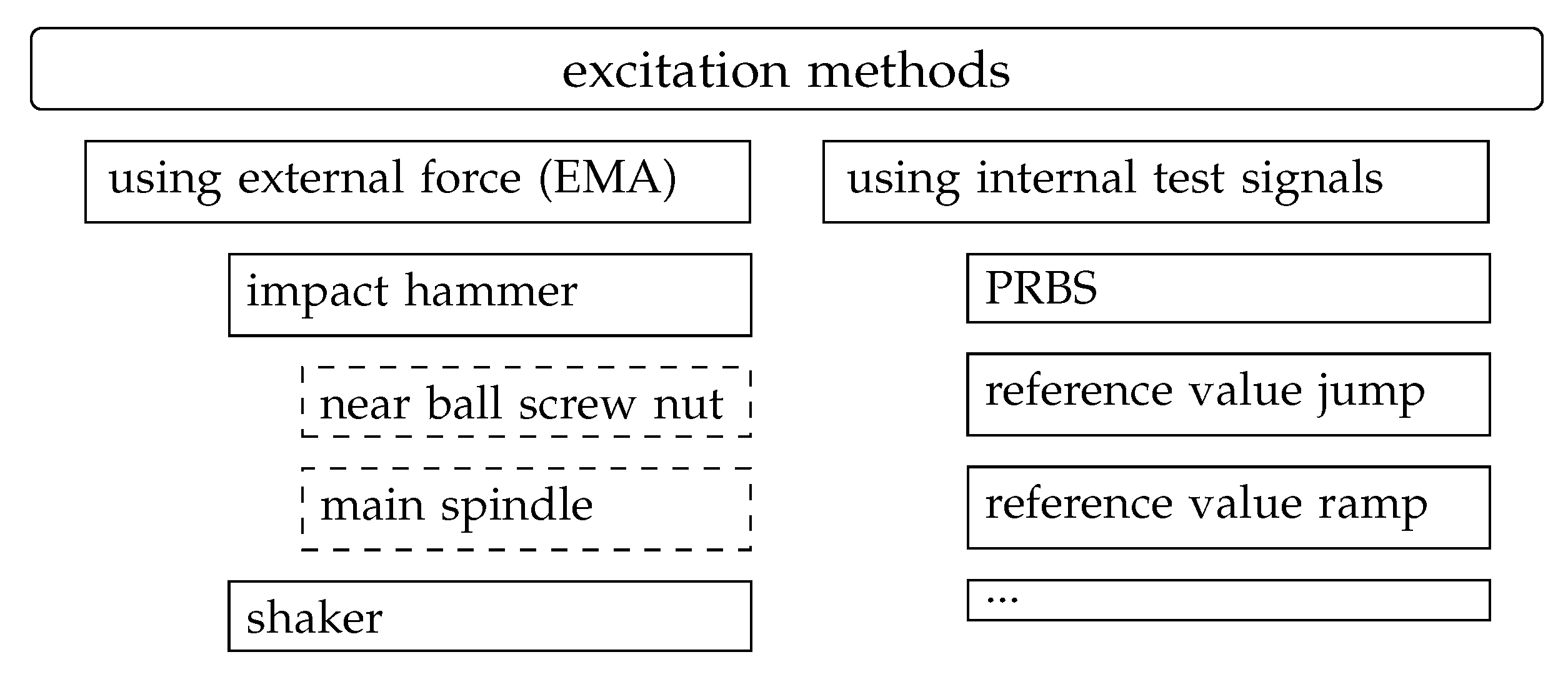
2.4. Strategies for Model Identification

The transfer functions and the TMF in Equation (5) can be identified via experiments. This is very efficient and more accurate compared to the calculation of the transfer functions and TMFs based on FE simulations or other models. In a first step, an appropriate excitation strategy is necessary. A broadband excitation of the mechanical structure at the TCP and at the drives is needed. In principal, there are two options, which are shown in Figure 2. On the one hand, an internal test signal, which is applied to the drive, could be used. Typically, this is realized by a pseudo random binary sequence (PRBS) in the commanded position. On the other hand, an external force to excite the machine could be used. Here, existing approaches from experimental modal analysis, e.g., impact testing via an impact hammer, can be used. A third alternative is the operational modal analysis [20,21,22]. The transfer functions $H_{TT}$ and $H_{ET}$ can be obtained by excitation at the TCP, e.g., via an impact hammer, and measuring the response with an accelerometer at the TCP and at the linear encoder, respectively. In general, at least one temporarily installed external sensor is necessary to measure the response at the TCP. Since the signals of the machine’s internal and external sensors are not easy to synchronize (sampling rate, start and end time may differ), the usage of two similar sensors at the TCP and the encoder position is advantageous. By using data from two synchronized signals, the quality of the TMF is less noisy and the phase of the TMF is more accurate (no artificial time shift).

For the identification of the TMF $T_{TE}^D\left(s\right)$, it is important to keep in mind that the TMF depends on the location of the excitation. To illustrate this, the TMFs for a oscillator chain with three masses have been plotted in Figure 3. Three mass oscillators are a simplified model for the dynamic behaviour of a machine tool drive [23]. From this example, one can observe that the TMF $T_{32}^1\left(j\omega \right)$ is identical to $T_{32}^2\left(j\omega \right)$, whereas $T_{32}^3\left(j\omega \right)$ differ from the two former ones. This is due to the fact that for the identification of a transmissibility function between mass 2 and mass 3 it is not important if the excitation occurs directly at position 2 or at position 1, which is on the same side of the oscillator chain. For the machine tool drive and the identification of $T_{TE}^D$, this means that an excitation near the encoder position, e.g., with an impact hammer, is comparable to the excitation at the drive for example with an internal PRBS signal for the commanded position. In contrast, an excitation at the TCP would lead to wrong results for $T_{TE}^D$ because the excitation must be on the side of the drive.

This theory is validated via measurements at the x-axis of a 5-axis milling machine. Figure 4 shows the TMFs $T_{TE}^D$, $T_{TE}^E$, $T_{TE}^T$ between the encoder position and the TCP position for three different locations of the excitation, i.e., excitation at the drive (D) via a PRBS signal (black curves in Figure 4), excitation near the encoder (E) via an impact hammer (green curves) and hammer excitation at the TCP (T, black curves).

The response was measured via piezo-electric accelerometers whose position was not changed. In accordance with the theory and the results from the three mass oscillator in Figure 3, the TMF $T_{TE}^D\left(j\omega \right)$ is similar to $T_{TE}^E\left(j\omega \right)$ because the excitation is on the drive side. In contrast, the TMF $T_{TE}^T\left(j\omega \right)$ deviates significantly from the other two TMFs because in this case the excitation occurs on the TCP side.

3. Results

3.1. Measured Transmissibility Functions

To identify the TMF $T_{TE}^D\left(j\omega \right)$, a external acceleration sensor at the TCP is placed. The second relevant point is the linear position encoder. Here, an existing linear position encoder could be used. With the accelerometer, the transfer behavior at very low frequencies cannot be measured. However, the mechanical structure is similar to a low pass filter and at very low frequencies the TCP position follows by one-to-one the encoder position. There is also the possibility to place an external acceleration sensor near the encoder location. The second option has different advantages. Firstly, the analysis of the measured data is easier, because both signals can be captured with the same data acquisition system. This means that there is no time-shift, no difference between the sampling rates of the signals and no integration differentiation of the signals is necessary. Secondly, the measurement range is higher. There is no need to limit the range to the sampling rate of the machine control (about 500 Hz). If the excitation force is wide banded enough, higher frequency modal parameters of the machine can be respected.

Figure 5 shows measurement results for the two measurement options. An accelerometer was placed close to the linear encoder of the drive (observe the left side in Figure 5). The machine was excited with a hit of an impact hammer at the TCP. One can observe that both signals are close to each other in the frequency range between 20 Hz and 160 Hz. In this case, the sampling rate for the encoder signal was 3 ms, which sets the upper frequency limit due to the Nyquist criterion. At very low frequencies, the signal of the accelerometer is not reliable and diverges compared to the encoder signal. However, with the accelerometer, signals at higher frequencies (compared to the 166 Hz limit of the encoder) can be also obtained. The slight difference between the encoder signal and the accelerometer signal at frequencies between 100 Hz and 120 Hz is probably due to the slight difference in the location of the encoder and the accelerometer.

3.2. Position Depending Dynamic Behaviour of Machine Tools

Dependent on the machine tool concept the dynamic behavior at the TCP depends on the position of the feed axes. Some examples for regular transfer function can be found in [20,21,24,25]. For the feed drive closest to the TCP the approach in Equation (6) mainly eliminates position-dependent behavior of the TMFs. However, this does not hold in general. Figure 6 shows an example for position-dependent TMFs $T_{TE}^D$ for a 5-axis milling machine. In this case, the y-axis is mounted on a column, whereas the x-axis moves the column (see left side in Figure 6). Obviously, the behavior of the TMFs $T_{TE}^D$ in the x-direction depends on the position of the y-axis. This can be observed in the TMFs at the right side of Figure 6. In particular, the x-drive was excited via a PRBS signal and the TMFs was determined from the acceleration data at the TCP and near the linear position encoder. It can be observed that the TMFs vary depending on the position of the y-axis.

3.3. Modal Fitting

Figure 7 shows two approaches to transfer the experimental data into a model. The experimental modal analysis is a wide spread method to identify the modal parameters of cutting machine tools [26]. Here, classical transfer functions were measured in the frequency domain. Modal parameters (resonance frequency, modal damping and modal mass) were identified for each classical transfer functions, and the TMF was created from these modal parameters.

Figure 8 shows that method. The two frequency response functions (FRFs) $H_{TE}\left(j\omega \right)$ and $H_{EE}\left(j\omega \right)$ were obtained from impact hammer tests (black curves). The results from the modal fitting (green curves) coincide well with the measured FRFs. On the right side of Figure 8, the TMFs generated from the measurement data (black) and from modal parameters (green) are shown. The TMF from the modal fit is relatively close to the measured data. As an alternative way, the coefficients for a transfer function model from the measured inputs and outputs of the TMFs can be identified directly. In this case, a separate algorithm is necessary, since TMFs differ from regular transfer functions. For example, the numerator and denominator of the transfer function can have the same order, which does not hold for typical transfer functions for displacements in response to force. As an advantage of the second approach, the resulting TMFs are typically more precise because the measured input and output data of the TMFs are directly used for the model identification and a general transfer function model allows more freedom in the parametrization.

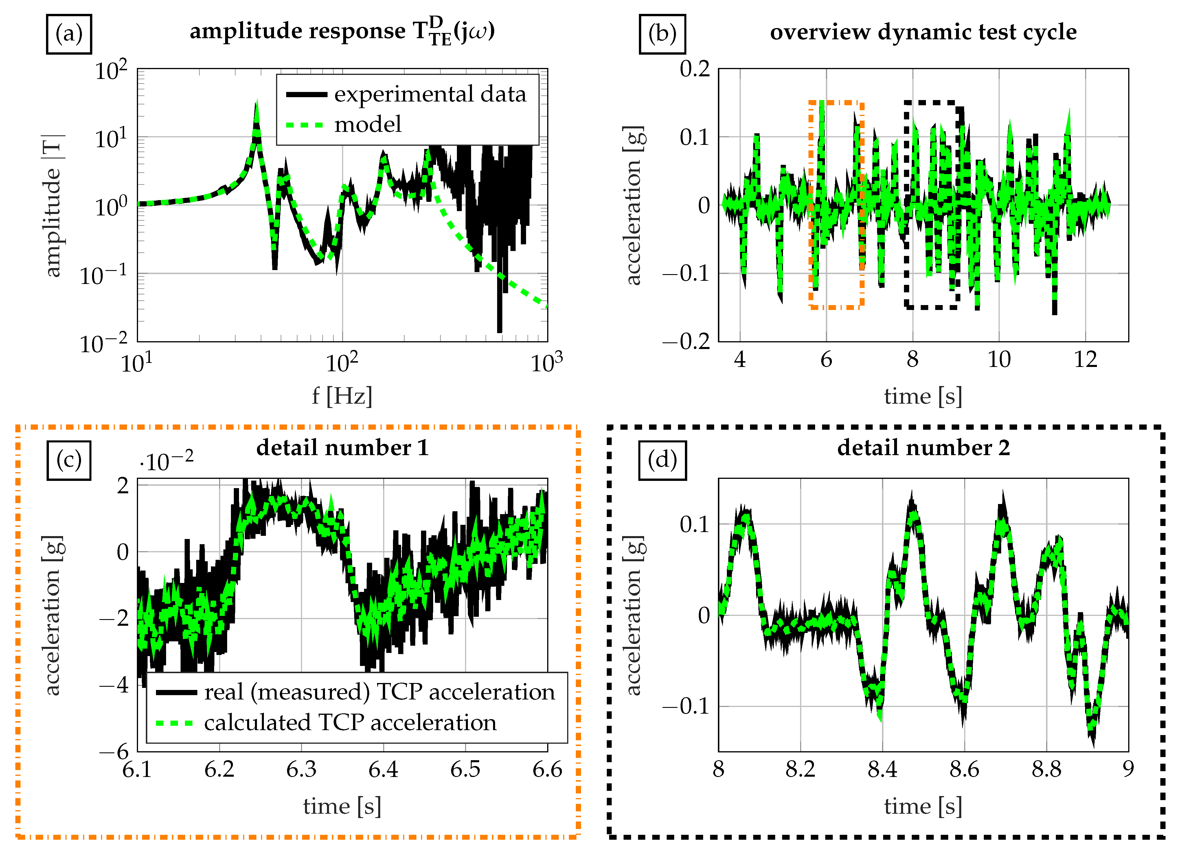
3.4. Verification of the Results

The performance of the VS is tested for a dynamic test cycle on a 5-axis milling machine. Here, only results for the x-direction are demonstrated, but similar behavior is found for the other directions. The measured and fitted TMF is shown in Figure 9a. An excitation at the drive with a PRBS signal was used for the experimental identification. This means that an excitation up to a frequency of up to 330 Hz occurs (servo cycle time 3 ms). The encoder and TCP motion was measured with two accelerometers, with a bandwith up to 800 Hz. This means that the TMFs can be reliably identified up to 333 Hz. In this frequency range the fitted TMF coincide well with the measured data. An overview over the test cycle and the corresponding accelerations at the x-axis are shown in Figure 9b.

A detailed comparison between the measured signal (black) and the outcome of the VS (green) is shown in Figure 9c,d. The virtual sensor performs very good for the low frequency area, whereas some deviations occur for high frequency behavior. This is because excitation at high frequencies was missing during the model identification of the VS, and therefore, the bandwidth of the VS (333 Hz) is lower than the bandwidth of the accelerometer (800 Hz).

4. Discussion

The test cycle has demonstrated that the VS works as expected in the considered frequency range. Deviations at high frequencies occur, because the TMF was identified by using an excitation via machine internal PRBS signals. The PRBS signal is limited to the servo cycle time of the position control system of the machine, and therefore, does not excite higher frequencies. The presented approach is a very general one, and can be applied to different types of CNC machines. The measurement strategy has to be adjusted slightly depending on the structure of the machine, the control system and the number of CNC axes. An external impact or internal test signal could be used to excite the machine from the drive side. For measuring the response at the TCP and encoder locations, only external or a combination of external and internal sensors can be used. When using separate external sensors near the encoder of the drives, the signals are slightly different compared to the data of the internal machine sensors. However, these deviations are small and can be neglected. The performed test cycle compares two accelerations and was only performed for one axis.

In future work, other testing methods for measuring the position of the TCP are needed. Moreover, the concept of the virtual sensor needs to be improved for also considering the geometric behavior of the machine tool. Geometric failures can lead to dominant contour errors at the work piece. In addition to the considered dynamic contour errors and geometric errors, the effect of cutting forces can be taken into account, which is already considered in the theoretical part, see, e.g., Equation (5). However, in practice, the determination of the cutting force during the process without extensive measurement effort is not possible. One approach could be to also identify the cutting force via a virtual sensor or state observer based on the machine internal data [17,18].

5. Conclusions

This article demonstrates an approach for using virtual sensors for accuracy monitoring in CNC machines. The virtual sensor can be used for process optimization, monitoring of the accuracy of machine tools or anomaly detection. The identification of the modeling part of the VS sensor can be conducted efficiently with standard experiments and only a few additional external sensors. The model is based on transmissibility functions (TMFs). This special transfer functions makes it possible to use the high quality data of the linear position encoder of CNC machines as an input for the VS. Some important aspects, which are relevant for the experimental identification and the model generation, were presented. The results are verified for data from the X-axis of a milling machine based on a dynamic test cycle. It was demonstrated that the virtual sensor works properly in the relevant frequency range.

The novelty of the approach lays in the usage of TMFs to calculate dynamical derivations at the TCP from internal machine sensor data for a running machine. This is a key difference to existing approaches for contour error prediction based on simulations before the real process. Ideally, the signal from the virtual sensor of the presented approach is equivalent to a position sensor at the tool center point with the advantage that no additional sensor is required. The usage of internal sensor signals reduces the overall cost and complexity of the system. This approach provides a contribution to the real-time accuracy monitoring of CNC machines. With this application, a system for optimal process planning and monitoring, while ensuring minimal cost and effort, could be created.

References

1. Altintas, Y.; Brecher, C.; Weck, M.; Witt, S. Virtual Machine Tool. CIRP Ann. 2005, 54, 115–138. [Google Scholar] [CrossRef]
2. Brecher, C.; Wellmann, F.; Epple, A. Quality-predictive CAM Simulation for NC Milling. Procedia Manuf. 2017, 11, 1519–1527. [Google Scholar] [CrossRef]
3. Haenel, A.; Seidel, A.; Friess, U.; Teicher, U.; Wiemer, H.; Wang, D.; Wenkler, E.; Penter, L.; Hellmich, A.; Ihlenfeldt, S. Digital Twins for High-Tech Machining Applications—A Model-Based Analytics-Ready Approach. J. Manuf. Mater. Process. 2021, 5, 80. [Google Scholar] [CrossRef]
4. Altintas, Y.; Kersting, P.; Biermann, D.; Budak, E.; Denkena, B.; Lazoglu, I. Virtual process systems for part machining operations. CIRP Ann. 2014, 63, 585–605. [Google Scholar] [CrossRef]
5. Biermann, D.; Surmann, T.; Kersting, P. Oscillator-based approach for modeling process dynamics in NC milling with position- and time-dependent modal parameters. Prod. Eng. 2013, 7, 417–422. [Google Scholar] [CrossRef]
6. Großmann, K.; Loeser, M. Einflussgroessen auf die Stabilitaet von Zerspanprozessen eine vergleichende Untersuchung. ZWF 2011, 106, 147–152. [Google Scholar] [CrossRef]
7. Otto, A.; Rauh, S.; Kolouch, M.; Radons, G. Extension of Tlustys law for the identification of chatter stability lobes in multi-dimensional cutting processes. Int. J. Mach. Tools Manuf. 2014, 82, 50–58. [Google Scholar] [CrossRef]
8. Zhou, Y.; Xue, W. Review of tool condition monitoring methods in milling processes. Int. J. Adv. Manuf. Technol. 2018, 96, 2509–2523. [Google Scholar] [CrossRef]
9. Mohanraj, T.; Shankar, S.; Rajasekar, R.; Pramatik, A. Tool condition monitoring techniques in milling process—A review. J. Mater. Res. Technol. 2020, 9, 1032–1042. [Google Scholar] [CrossRef]
10. Barton, D.; Federhen, J.; Fleischer, J. Retrofittable vibration-based monitoring of milling processes using wavelet packet transform. Procedia CIRP 2021, 96, 353–358. [Google Scholar] [CrossRef]
11. Madhusudana, C.K.; Kumar, H.; Narendranath, S. Condition monitoring of face milling tool using K-star algorithm and histogram features of vibration signal. Eng. Sci. Technol. Int. J. 2016, 19, 1543–1551. [Google Scholar] [CrossRef] [Green Version]
12. Liu, M.; Liang, S.Y. Analytical modeling of acoustic emission for monitoring of peripheral milling process. Int. J. Mach. Tools Manuf. 1991, 31, 589–606. [Google Scholar] [CrossRef]
13. Becker, T.; Krause, D. Softsensorsysteme - Mathematik als Bindeglied zum Prozessgeschehen. Chem. Ing. Tech. 2010, 82, 429–440. [Google Scholar] [CrossRef]
14. Dementjev, A.; Hensel, B.; Kabitzsch, K.; Kauschinger, B.; Schroeder, S. Virtual Sensor for Calibration of Thermal Models of Machine Tools. Adv. Artif. Neural Syst. 2014, 2014, 347062. [Google Scholar] [CrossRef] [Green Version]
15. Erwinski, K.; Paprocki, M.; Wawrzak, A.; Grzesiak, L.M. Neural network contour error predictor in CNC control systems. In Proceedings of the 2016 21st International Conference on Methods and Models in Automation and Robotics (MMAR), Piscataway, NJ, USA, 29 August–1 September 2016; pp. 537–542. [Google Scholar] [CrossRef]
16. Tieng, H.; Yang, H.C.; Hung, M.H.; Cheng, F.T. A novel virtual metrology scheme for predicting machining precision of machine tools. In Proceedings of the IEEE International Conference on Robotics and Automation, Karlsruhe, Germany, 6–10 May 2013; pp. 264–269. [Google Scholar] [CrossRef]
17. Yamada, Y.; Kakinuma, Y. Sensorless cutting force estimation for full-closed controlled ball-screw-driven stage. Int. J. Adv. Manuf. Technol. 2016, 87, 3337. [Google Scholar] [CrossRef]
18. Aslan, D.; Altintas, Y. Prediction of Cutting Forces in Five-Axis Milling Using Feed Drive Current Measurements. IEEE/ASME Trans. Mechatronics 2018, 23, 833–844. [Google Scholar] [CrossRef]
19. Maamar, A.; Le, T.P.; Gagnol, V.; Sabourin, L. Modal identification of a machine tool structure during machining operations. Int. J. Adv. Manuf. Technol. 2019, 102, 253–264. [Google Scholar] [CrossRef]
20. Berthold, J.; Kolouch, M.; Wittstock, V.; Putz, M. Identification of modal parameters of machine tools during cutting by operational modal analysis. Procedia CIRP 2018, 77, 473–476. [Google Scholar] [CrossRef]
21. Berthold, J.; Kolouch, M.; Regel, J.; Putz, M. Investigation of the dynamic behavior of machine tools during cutting by operational modal analysis. MM SJ (MM Sci. J.) 2019, 2019, 3078–3085. [Google Scholar] [CrossRef]
22. Zaghbani, I.; Songmene, V. Estimation of machine-tool dynamic parameters during machining operation through operational modal analysis. Int. J. Mach. Tools Manuf. 2009, 49, 947–957. [Google Scholar] [CrossRef]
23. Gross, H.; Harmann, J.; Wiegaertner, G. Elektrische Vorschubantriebe in der Automatisierungstechnik: Grundlagen, Berechnung, Bemessung; Publicis: Paris, France, 2006. [Google Scholar]
24. Law, M.; Ihlenfeldt, S.; Wabner, M.; Altintas, Y.; Neugebauer, R. Position-dependent dynamics and stability of serial-parallel kinematic machines. CIRP Ann.-Manuf. Technol. 2013, 62, 375–378. [Google Scholar] [CrossRef]
25. Brecher, C.; Altstädter, H.; Daniels, M. Axis Position Dependent Dynamics of Multi-axis Milling Machines. Procedia CIRP 2015, 31, 508–514. [Google Scholar] [CrossRef]
26. Natke, H. Einführung in Theorie und Praxis der Zeitreihen- und Modalanalyse Schwingungsfähiger Elastomechanischer Systeme; Vieweg: Braunschweig, Germany, 1992. [Google Scholar]
Figure 1. (a) Overview about the relevant dynamical parts of a milling machine axis. (b) Principal functionality of a virtual sensor.
Jmmp 06 00137 g001
Figure 2. Overview about the excitation methods.
Jmmp 06 00137 g002
Figure 3. Theory of TMFs shown on a simple dynamic system.
Jmmp 06 00137 g003
Figure 4. TMF for different points of excitation (experimental results).
Jmmp 06 00137 g004
Figure 5. Comparison of double-integrated acceleration and internal position signal.
Jmmp 06 00137 g005
Figure 6. Position depending behaviour of T T E D ( j ω ) .
Jmmp 06 00137 g006
Figure 7. Generation of transmissibility functions.
Jmmp 06 00137 g007
Figure 8. TMF build out of two regular FRFs.
Jmmp 06 00137 g008
Figure 9. (a) measured and fitted TMF, (b) overview over the test cycle and the corresponding accelerations, (c) detailed comparison between the measured signal (black) and the outcome of the VS (green), (d) detail 2.
Jmmp 06 00137 g009
Publisher’s Note: MDPI stays neutral with regard to jurisdictional claims in published maps and institutional affiliations.