Calibration of Finite Element Model of Titanium Laser Welding by Fractional Factorial Design

Abstract

This paper focuses on the calibration of heat source parameters to reproduce temperatures and distortions in welded joints. Specifically, the proposed methodology, which combines the Finite Element Method and Design of Experiments, is applied to calibrate a T-joint dissimilar titanium laser welding process. The thermal problem is addressed using a 3D transient model with a Conical Gaussian heat flux, and the mechanical problem is tackled using a 3D elastic-plastic model. A Fractional-Factorial Design is performed to define a set of thermo-mechanical uncoupled models. Finally, optimal parameter combinations that replicate experimental data are identified. This methodology allows automation that replaces the traditional trial and error process, which frequently does not provide good results, is an exhausting task and requires a dubious amount of time.

1. Introduction

Hybrid Laminar Flow Control (HLFC) on fins and wings is a key to improving aircraft efficiency, whereby fuel savings of up to 10% can be achieved [1]. The HLFC concept relies on suctioning air through a micro-drilled skin, which gives rise to an enlargement in laminar flow on the surface of the leading edges. Using Laser Beam Welding (LBW) in the aerospace industry offers substantial cost and weight savings compared to conventional joining methods [2,3,4]. LBW is a manufacturing process for joining metal pieces using the energy provided by a laser beam to melt the materials to be joined. LBW process parameters, such as laser power, welding speed, focal position, and shielding, must be identified to produce high-quality welds. A laser beam is a monochromatic, directional, and coherent light with a single wavelength. Its high power density can be reached by focusing the beam on a very small spot, which can be at a great distance because of the low divergence of the beam [5]. There are two modes of LBW based on power density: keyhole mode and conduction mode. It is performed in keyhole mode when the power beam density is high enough to melt and vaporize the material. In contrast, conduction mode is implemented when the power density cannot vaporize the materials but is high enough to melt them superficially. In this case, the heat from the laser is absorbed by the workpiece surface and transferred inside the workpiece through conduction. Deep penetration is impossible in this case because it is limited by the thermal conductivity of the materials being welded [6].

Measurements of welding temperatures, distortions, and residual stresses require high experimental effort and are very time-consuming. As a result, numerical modelling methods, including the Finite Element Method (FEM), are often used to predict the residual stresses and distortions during and after welding. FEM is flexible and less expensive in comparison to experimental methods and has proved to be an efficient tool for simulating the welding process and subsequent deformation of structures [7,8,9]. Additionally, a finite element analysis (FEA) makes it possible to gain a better understanding of the thermomechanics of welding processes. A considerable number of research articles about predicting welding residual stresses and distortions performed by means of FEM have been published in the last decades. Ueda and Yuan [10], Hibbitt and Marcal [11], and Friedman [12] published some of the earliest FEM models developed to predict distortions and residual stresses generated during the welding process. These models contained simplifications due to computing power limitations, including two-dimensional analyses of normal sections. Prediction of welding residual stresses and distortions depends on the accurate determination of temperature distribution, which requires a nonlinear transient 3D analysis [13]. Detailed 3D FEM models are still computationally too expensive to analyze large structures, and therefore simplifications are frequently required. Comprehensive literature reviews of welding simulation methods were produced by Lindgren [14,15,16] and He [17].

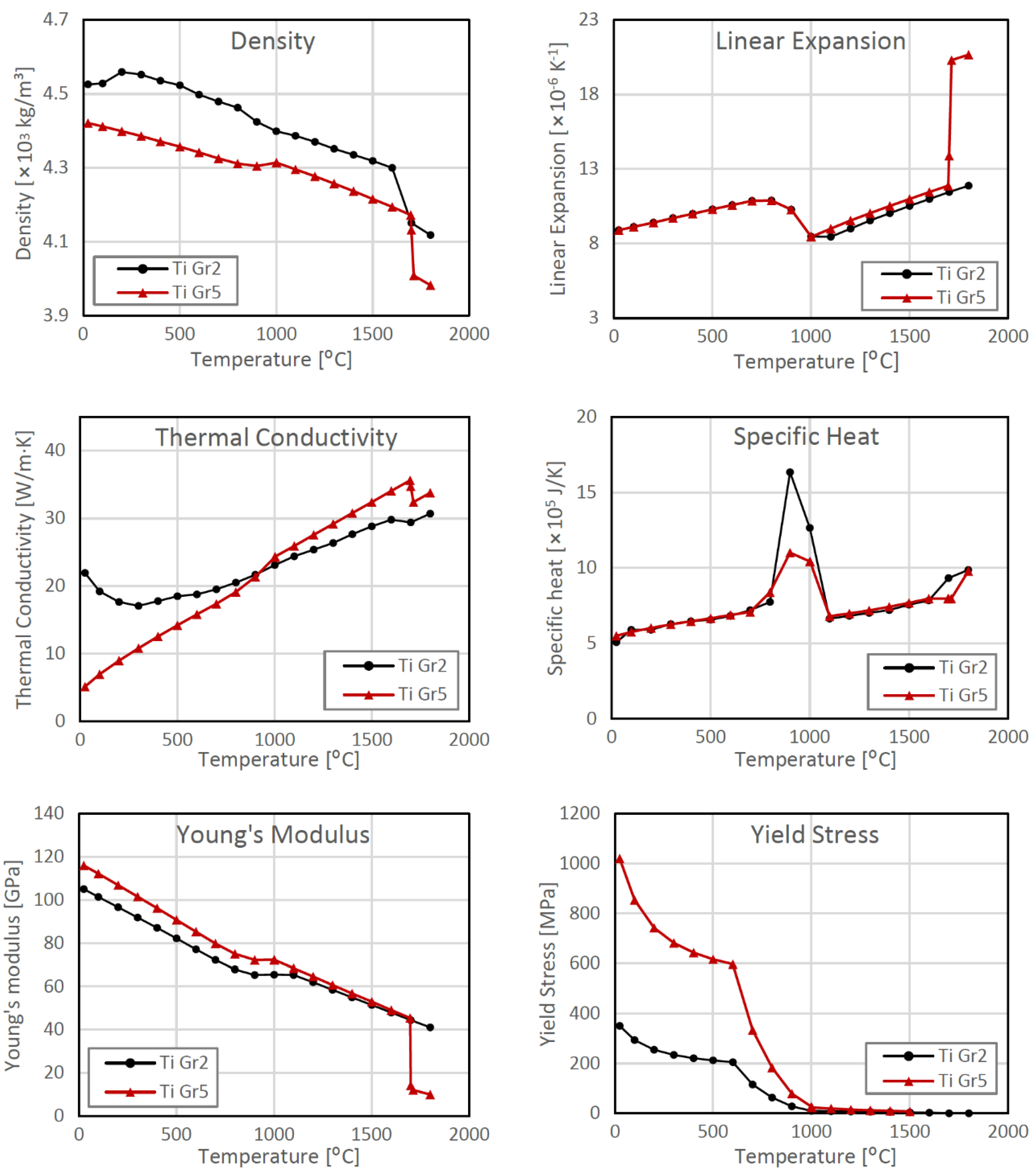
Material properties, heat source, and realistic boundary conditions are essential to get accurate predictions of a welding process. Zhu and Chao [18] investigated the importance of temperature-dependent material properties in a FEM simulation of an aluminum welding process. The temperature-dependent material properties, such as yield strength, were calculated as linear functions of temperature, where the material properties obtained at room temperature were included. The modeling results were in good agreement with the experimental results

The first moving heat source model was proposed by Rosenthal for a point and a line [19,20], but it yields large errors in predicting the temperature field. Pavelic et al. [21] developed surface heat flux with Gaussian distribution; however, this model is only effective for low power densities and reduced penetration. Goldak et al. [22] modeled the heat flux with a volume defined by a double ellipsoidal and Gaussian distribution to overcome the problems with the low penetration of previous models. Aissani et al. proposed an alternative model to the Goldak heat input for Tungsten Inert Gas welding (TIG) based on a Gaussian surface source exhibiting a bi-elliptical shape [23]. These models are widely used for electric arc processes [24,25,26,27]; nevertheless, a conical model with a Gaussian radial distribution and an axial linear distribution produces more accurate results for LBW [21]. 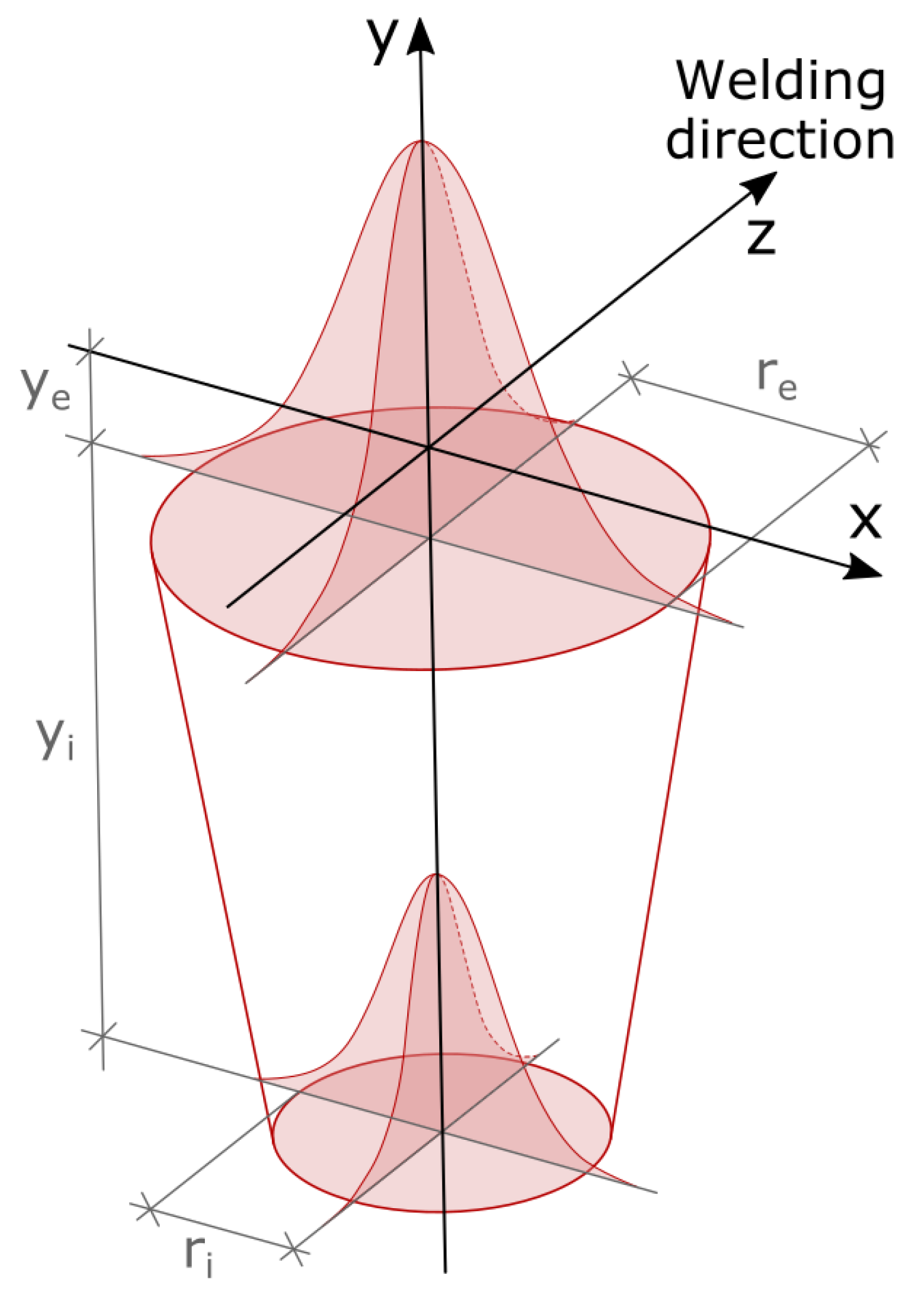This heat flux model has been successfully used to simulate titanium laser beam welding [28,29,30]. The conical Gaussian heat flux is calculated with the following equations:

$$r_0=r_e-\left(r_e-r_i\right)·\frac{y_e-y}{y_e-y_i}$$

(1)

$$\mathrm{Q}\left(x,y,z\right)=\frac{9·\eta ·P·\exp \left(-9·\left(x^2-z^2\right)/r_0^2\right)}{\mathsf{\pi }·\left({\mathrm{e}}^3-1\right)·\left(y_e-y_i\right)·\left(r_e^2+r_e·r_i+r_i^2\right)}$$

(2)

where P is the laser power, (x, y, z) are the coordinates of the node, η is the process efficiency, and r_e, r_i, y_e, and y_i are the dimensions of the cone shown in Figure 1. Distortions, residual stresses, and a heated volume during LBW were numerically simulated by taking into consideration thermal and mechanical boundary conditions. The present paper describes the multi-objective fitting procedure to find the unknown thermal condition that accurately simulates an LBW process.

The heat source parameters found in this study were used to simulate distortions in large HLFC structures using an inherent strain method. This approach described by Mendizabal [31] claims that welding distortions can be solved using an elastic model to apply the plastic strain field in the weld bead and surrounding area. In practice, it means extracting the plastic strains from a small transient analysis as the input for the inherent strain analysis. This method has been applied to calculate distortions with good computational efficiency in large and complex components [10,32,33]. The inherent strain method, which is not included in this paper, was implemented in the project DELASTI, supported by the European Commission (grant agreement no: 687088). That project aimed at developing manufacturing processes and system technology for reproducible LBW and laser straightening of titanium structures for HLFC Technology.

2. Materials and Methods

2.1. Experimental Data Acquisition

Dissimilar LBW joint between commercially pure titanium (ASTM Grade 2) and Ti-6Al-4V alloy (ASTM Grade 5) in a T-joint configuration was simulated [34]. Both materials were provided as sheets of 0.8 mm in thickness. Ti-Gr2 [35] has good weldability, corrosion resistance, and a minimum yield strength of 275 MPa. Ti-Gr5 [36] has very good mechanical properties up to 400 °C, with a yield strength higher than 1000 MPa. Because of its vanadium and aluminum content, it belongs to (α + β) titanium alloys, which makes it possible to obtain various microstructures depending on the working parameters. The combination of the high corrosion resistance of the Ti-Gr2 skin and the high strength of Ti-Gr5 stringer creates structures with excellent mechanical properties that fulfill the strict regulations of the aircraft industry [37].

Experimental data were acquired using specimens of 100 mm length to validate FEM model predictions. These data consist of micrographs of the molten weld pool, temperatures at controlled points in time, and angular distortions after welding and straightening. The data were obtained keeping constant the parameters of the welding process summarized in

Table 1. Welded sample: manufacturing parameters.

Profile	Value
Power	700 W
Focal lens	200 mm
Focal spot diameter	400 µm
Center wavelength	1030 µm
Laser beam inclination	25°
Speed	3.5 m/min
Offset	0.4 mm

. Welding source was a disk laser of type Trudisk 5002 (6C) mounted on a Gantry KUKA RLP60-60 robot.

Thermocouples were welded to experimental samples to record temperature evolution in four points during and subsequent cooling, as shown in Figure 2. Data were recorded using an MX100 Data Acquisition Unit and software from YOKOGAWA company. The recorded results are presented in Figure 3.

The welded joint was cut and metallographically prepared to obtain the melt pool area. After the cut, the faces were ground using decreasing grind paper sizes (from 240 to 1200) and polished. Then, the specimen was etched with reactive Kroll (3% HF, 6%HNO₃, 91% distilled water). Once the specimen was prepared, it was analyzed under the microscope Olympus GX 51 with 100× magnification. Figure 4 shows weld pool shape and Heat-Affected Zones (HAZ) of both Ti-Gr2 skin and Ti-Gr5 stringer.

Finally, welded samples were positioned on an even surface to measure distortions, as shown in Figure 5. The data were acquired using a SCANSONIC optical sensor (TH6i-150-CF). Laser triangulation concept was employed for measuring angular distortions on the reverse of the skin through some paths, which were perpendicular to the welded stringers (X-axis). Along these paths, vertical height of the sample was measured (Z component of distortion). Angular distortion was then calculated along each path using a linear regression, calculated through minimum squares, between points on the left of the weld and on the right. Angular distortions were measured in five profiles separated by 20 mm between them, beginning at 10 mm from the edge.

The angular distortion calculation procedure, applied independently to each profile, consists of the following steps:

• Determination of the central peak.
• Splitting the measurement points into two groups: from the first point to the peak (to the left of the central peak) and from the peak to the last one (to the right of the central peak).
• Fitting a linear regression model for each group using minimum squares:

z₂ = a₂ + b₂∙x

(3)

z₂ = a₂ + b₂∙x

(4)

4.

Calculation of the line angle by applying the following equation:

A = atan (b₁ − b₂)

(5)

The measured Z component of distortion and calculated angular distortion for each profile after LBW of one sample are shown in Figure 6 and

Table 2. Welded sample: angular distortions.

Profile	Welding Angle
Profile 1	1.37°
Profile 2	1.27°
Profile 3	1.27°
Profile 4	1.34°
Profile 5	1.31°
Average	1.31°

.

2.2. FEM Model

Uncoupling the welding process into sequential thermal transient and elastic–plastic analyses provides good results, minimum accuracy loss, and computational time reduction [13,15,38]. This is possible because the heat generated by plastic deformation in the process is negligible compared to the heat generated by the welding heat source [11,39,40]. Therefore, an uncoupled analysis was applied to tackle thermal and mechanical behavior. Export/import options available in Abaqus were used to transfer the field of temperatures from thermal to mechanical analysis.

Both analyses had the same geometry, mesh, and physical properties. The dimensions of both models were 80 × 20 × 50 mm with thicknesses of 0.8 mm and were developed with Abaqus [41], as shown in Figure 7. For the thermal model, elements DC3D8 (0.1 mm size) were used in the regions near the weld bead and elements DC3D6 (2.5 mm size) in areas further away. In this way, the model is composed of elements. Similarly, elements C3D8 and C3D6 were used in the mechanical model. The material of the skin (horizontal plate) is Titanium Grade 2, while the stringer (vertical plate) is Titanium Grade 5. Isotropic elastoplastic constitutive models with temperature dependence were used. Thermo-mechanical properties of both alloys, depending on temperature, were obtained from JMatpro [28,29,42]. Young’s modulus, yield strength, and thermal expansion of Ti-Gr2 have been calculated based on Ti-Gr5 properties and data provided in the literature [43,44]. Temperature-dependent material properties that were employed in the FEM models are summarized in Figure 8. Other bibliographic resources [45] were considered to define the thermo-mechanical properties of both Ti alloys, including temperature-dependent and constant physical properties, but they were discarded due to the lack of accuracy in the FEM predictions.

In the thermal model, the welding speed was 3.5 m/min (58.3 mm/s), the room temperature was 25 °C, and the convection coefficient was 0.05 mW/mm². The center of the laser beam was applied on the stringer at 0.3 mm from the top surface of the skin, and the inclination of the beam was 25 degrees. The heat flux generated during the LBW process was implemented in keyhole mode using a Conical Gaussian model via user subroutine DFLUX. This model defined the heat flux volume by means of four parameters (r_e, r_i, y_i, and y_e), as shown in Figure 1. The welding sequence was a straight line with speed of 10 m/min defined by its XYZ coordinates in DFLUX. Temperatures at four nodes near the weld pool are recorded during the welding process and posterior cooling to compare with thermocouple measurements.

Realistic clamping conditions were taken into consideration in the mechanical model, as shown in Figure 7. First, a vertical force was applied on the top surface of the stringer. At the same time, the vertical displacement of the two parallel lines of nodes was restricted to simulate the contact between the skin and the working table. Later, the stringer top surface was encastered, and then the LBW process started. After the joint was welded (Step 3) and cooled (Step 4), all the restrictions and forces were released. Finally, the node’s displacements at the central section were measured to calculate the angular distortion following the same method used for experimental measurements.

2.3. Design of Experiments (DoE)

Nowadays, DoE has been used successfully to implement multi-objective optimizations of processes both experimentally and using FEM models. Ref. [46] applied RSM and data mining (DM) techniques separately to optimize a welded joint experimentally. They concluded that regression models obtained with RSM performed better than DM models. Ref. [47] also used RSM to optimize an arc-welded joint, obtaining a good solution with a small number of trials. Ref. [48] combined FEM models and RSM to determine optimal arc welding process parameters, confirming the effectiveness of the method with reduced time and cost.

DoE determined the combination, randomization, replication, and blocking of the variables to establish cause-effect relationships with a certain degree of confidence. However, in this case, the trials were finite element analyses; thus, there was no need for randomization, replication, and blocking.

A DoE was implemented to find the best conical Gaussian dimensions and efficiency that meet the experimental data. The factors were the unknown inputs of the conical Gaussian heat flux model as shown in

Table 3. DoE parameters: factors, ranges, and units.

Factor	Symbol	Range		Unit
		Min	Max
Cone top radius	re	0.4	0.7	mm
Cone bottom radius	ri	0.0	0.3	mm
Cone height	yi	0.8	1.2	mm
Process Efficiency	η	0.5	0.8

: efficiency η, cone top radius r_e, cone bottom radius r_i, and cone height y_i (see Equations (1) and (2)). Goldak parameter ranges were defined based on the micrograph (Figure 4), and the efficiency range was based on previous experience. Parameter y_e defined the position of the cone along the nozzle axis that was inclined 25° (see Figure 2b). This parameter is not a DoE factor because it is calculated based on the factor r_e to make the top of the cone tangent to the stringer surface. In this way, there were four factors, and therefore the number of combinations was 3⁴ = 81 considering three values per factor. This kind of design is called a full three-level design (or 3k) because it considers all possible combinations with three values, also called levels. However, 81 simulations were completely unaffordable, considering that one mechanical simulation took about 18 h (Intel Xeon E5-2690v3, 192 GB RAM, 12 CPUs). There are techniques, such as Central Composite Design [49] or Box-Behnken Design [50], that reduce the number of experiments to 24 and 25, respectively, which were also unaffordable. For all these reasons, Fractional-Factorial Design with resolution four ($4_{IV}^{4-1}$) and one central point was implemented. This design generated only 9 simulations, as shown in

Table 4. Fractional-Factorial Design.

Case	re	ri	yi	η
1	0.40	0.00	0.80	0.50
2	0.40	0.00	1.20	0.80
3	0.40	0.30	0.80	0.80
4	0.40	0.30	1.20	0.50
5	0.70	0.00	0.80	0.80
6	0.70	0.00	1.20	0.50
7	0.70	0.30	0.80	0.50
8	0.70	0.30	1.20	0.80
9	0.55	0.15	1.00	0.65

.

2.4. Response Surface Method (RSM)

RSM is a methodology that combines polynomial models and desirability functions [51]. The objective of RSM is to find the optimum working point using the minimum number of trials. First, FEM model results (temperatures and distortions) were gathered after all cases were simulated. Then, a polynomial model was adjusted for each output using the inputs and the results of the 9 cases:

$$Y=f\left(x_1,x_2,\dots ,x_n\right)$$

(6)

where Y is the calculated result, f is a polynomial function, and x_i are the inputs of the polynomial. Quadratic regression models are a polynomial function that is broadly used because it takes into consideration nonlinear effects and combined influence of inputs. The general form of the quadratic models is as follows:

$$Y=b_0+{\displaystyle \sum }_{i=1}^n{b}_i·x_i+{\displaystyle \sum }_{i=1}^n{b}_{ii}·x_i^2+{\displaystyle \sum }_{i=1}^{n-1}{\displaystyle \sum }_{j=i+1}^n{b}_{ij}·x_i·x_j+e$$

(7)

Because of the reduced number of levels of the Fractional-Factorial Design, it was not possible to determine quadratic terms. Thus, in this case, the polynomial model would be as follows:

$$Y=b_0+{\displaystyle \sum }_{i=1}^n{b}_i·x_i+{\displaystyle \sum }_{i=1}^{n-1}{\displaystyle \sum }_{j=i+1}^n{b}_{ij}·x_i·x_j+e$$

(8)

where b₀ is the independent term, the first summation is the linear term, the second one is the cross product of all input factors, and e is the error. Analysis of variance (ANOVA) can be used to evaluate the adjustment of the regression models to the experimental data. Responses can conflict with each other in a multi-objective optimization. It means that a solution can provide the optimal result for some objectives and poor results for the rest. In general, there is no unique solution that achieves all objectives at the same time. Instead, there are several Pareto-efficient solutions that cannot be improved in any objective without worsening other ones. This study uses expressions proposed by Harrington [51] to evaluate the overall response. The multi-objective optimization problem is formulated as:

Find r_e, r_i, y_i, and η to                    
Minimize geometric mean of errors T₁, T₂, T₃, T₄ and α    
Subject to 0.4 ≤ r_e ≤ 0.7, 0.0 ≤ r_i ≤ 0.3, 0.8 ≤ y_i ≤ 1.2 and 0.5 ≤ η ≤0.8

(9)

3. Results

Even the reduced number of simulations supposes too much computational time for the mechanical analyses, about 7 days using 12 CPUs. On the other hand, all thermal analyses were completed in only 24 h, also using parallel computing.

Table 5. FEM model results.

Case	T1 [°C]	T2 [°C]	T3 [°C]	T4 [°C]	α [°]
1	465.1	235.2	443.1	257.8	1.14
2	790.3	392.7	715.3	431.0	0.91
3	866.0	422.0	726.5	444.6	0.66
4	645.8	328.3	389.0	242.4	1.81
5	476.7	246.7	505.1	291.8	1.26
6	390.9	200.1	352.8	206.4	0.91
7	755.5	358.8	515.5	322.1	1.29
8	1212.0	583.3	668.2	436.8	0.41
9	421.9	212.3	375.6	220.7	1.01
Specimen	577	307	601	331	1.37

shows the maximum temperatures (thermal model) reached in four nodes that match the position of the thermocouples and the angular distortions from the mechanical model.

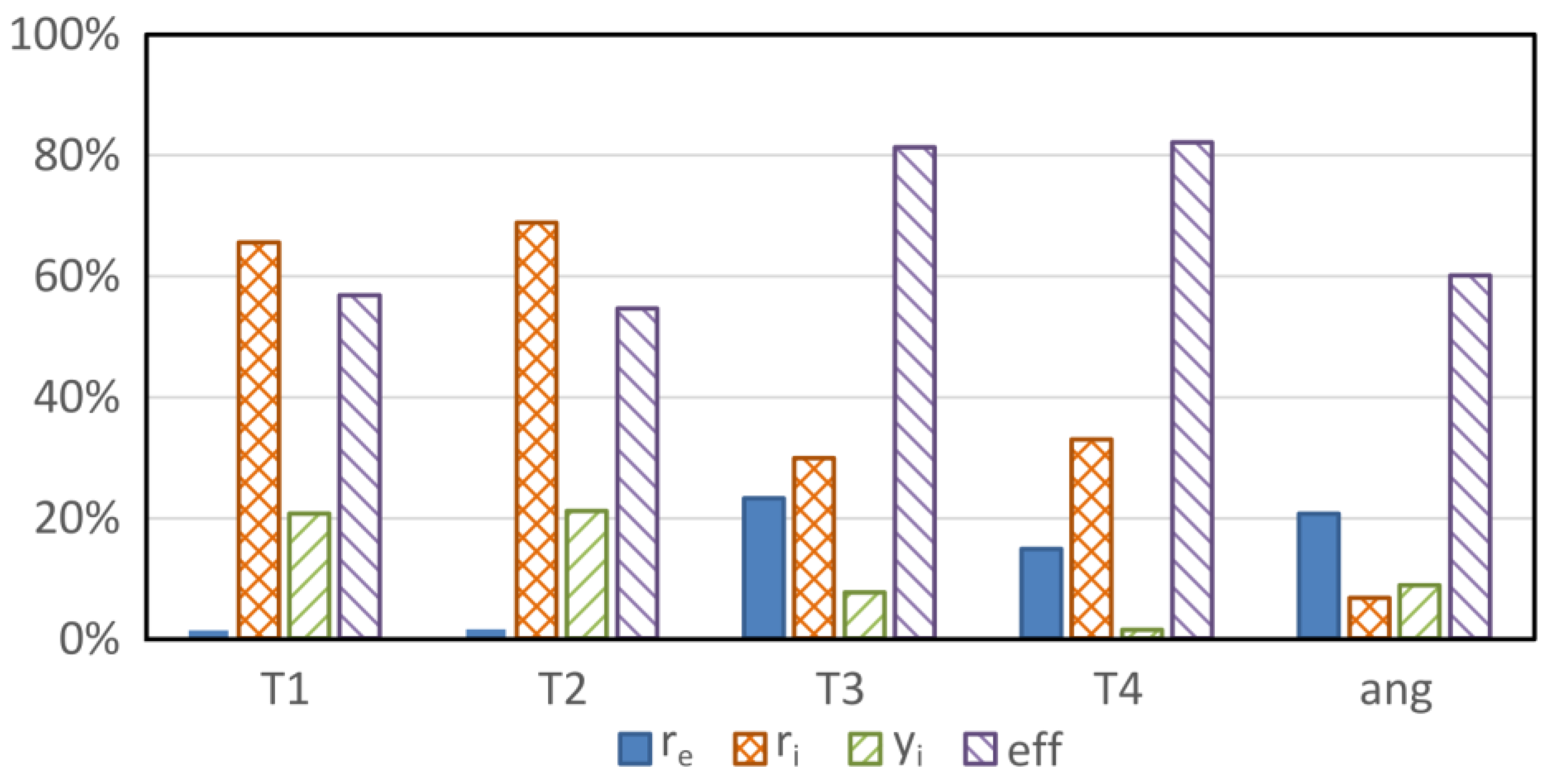
After all the simulations were completed, it was possible to study the influence of heat input parameters on the temperature and angular distortion. The correlations between the inputs and outputs (the results of the FEM models) are presented in Figure 9. The parameter Efficiency (Eff) has a high correlation with all the outputs, and it is the most important for three of them. This result is perfectly reasonable because higher efficiency implies more energy introduced into the joint, which leads to higher temperatures and larger distortions.

The bottom radius (r_i) has a high impact on temperatures T₁ and T₂, a moderate one on the other two, but very little on angular distortion. This fact relates directly to the location of the thermocouples: T₁ and T₂ are closer to the bottom of the heat cone than T₃ and T₄. Similarly, but conversely, the top radius (r_e) has more influence on T₃ and T₄. However, the effect of r_e on all temperatures is small. Finally, cone height (y_i) has more impact on T₁ and T₂ because a larger height means that the heat input penetrates more, which increases these two temperatures. Again, the effect of y_i on all temperatures is very small. These three cone dimensions have a small influence on angular distortion; its physical explanation is not clear.

Polynomials to predict model results were built using inputs and outputs (from Table 4 and Table 5) using the “R” statistical package [52]. These polynomials are:

$$\begin{array}{ll}{T}_1=& 729.5-2057.6·r_e-1264.6·r_i+945.7·\eta -449.4·y_i+4699.0·r_e·r_i\\ & +1348.7·r_e·y_i-227.6·r_i·y_i\end{array}$$

(10)

$$\begin{array}{ll}{T}_2=& -45.2-171.1·r_e-589.7·r_i+406.0·\eta +209.4·y_i+2122.3·r_e·r_i\\ & -148.7·r_e·y_i-65.8·r_i·y_i\end{array}$$

(11)

$$\begin{array}{ll}{T}_3=& 130.7-495.0·r_e+548.8·r_i+728.9·\eta +148.9·y_i-1334.7·r_i·y_i\end{array}$$

(12)

$$\begin{array}{ll}{T}_4=& -87.9-59.5·r_e+51.8·r_i+476.3·\eta +228.6·y_i+1441.2·r_e·r_i\\ & -242.4·r_e·y_i-653.6·r_i·y_i\end{array}$$

(13)

$$\begin{array}{ll}ang=& -2.04+8.70·r_e-0.52·r_i+3.97·y_i-1.55·\eta -5.33·r_e·r_i\\ & -8.43·r_e·y_i+3.28·r_i·y_i\end{array}$$

(14)

These polynomials were built using the minimum square method. These polynomials show how each output was defined by first-order terms and the cross-product of input factors. Then, ANOVA was used to reduce the size of these regression models by removing the non-significant terms by applying a step-wise algorithm [53].

p-values from ANOVAs prove that polynomials are statistically significant (

Table 6. ANOVA of the regression models.

Predictor	T1		T2		T3		T4		Ang
	Coef.	p-Value	Coef.	p-Value	Coef.	p-Value	Coef.	p-Value	Coef.	p-Value
Intercept	+729.5	0.0769	−45.2	0.3640	130.7	0.0643	−87.9	0.0452	−2.04	0.0271
re	−2057.6	0.0446	−171.1	0.0783	−495.0	0.0395	−495.0	0.1524	+8.70	0.0100
ri	−1264.6	0.0997	−589.7	0.0775	+548.8	0.0516	+548.8	0.0752	−0.52	0.2404
yi	−449.4	0.1220	+209.4	0.0190	+148.9	0.1990	+148.9	0.0208	+3.97	0.0125
η	+945.7	0.0213	+406.0	0.0227	+728.9	0.0103	+728.9	0.0045	−1.55	0.0104
re · ri	+4699.0	0.0260	+2122.3	0.1513	0.0	0.1453	+1441.2	0.0086	−5.33	0.0194
re · yi	+1348.7	0.0639	−148.7	0.2581	0.0	0.0711	−242.4	0.0265	−8.43	0.0099
ri · yi	−227.6	0.1808	−65.8	0.3640	−1334.7	0.0249	+653.6	0.0197	+3.28	0.0250
Model		0.039		0.029		0.019		0.012		0.020
R2	0.963		0.969		0.997		0.987		0.983
R2adj	0.906		0.928		0.989		0.971		0.954

). Additionally, the R-squared value (R²) is calculated to measure the amount of variation in the outputs that are explained by the inputs. The results show that all values of R² are close to 1, which indicates that these models possess a good predictive capacity. Now it was possible to find the optimum working point using desirability functions. Package “desirability,” available in “R,” was used to calculate the four temperatures, angular distortion, and overall desirability [54]. The determination of the working point with the maximum desirability was achieved by applying the steepest ascent method [55]. The objectives of the optimization and results of the optimization are summarized in

Table 7. Optimization objectives, results, and desirability.

	Objective	Result	Desirability
re	in range	0.41	1.00
ri	in range	0.29	1.00
yi	in range	0.78	1.00
η	in range	0.50	1.00
T1	576.7	565.4	0.94
T2	307.3	282.8	0.77
T3	601.4	490.7	0.55
T4	331.2	252.4	0.37
ang	1.37	1.41	0.91
Overall desirability			0.67

.

The optimal parameters from Table 7 were used to set a new simulation.

Table 8. Optimization results comparison.

	FEM Results	Experimental	Error
T1	548.9	576.7	5.1%
T2	272.4	307.3	12.8%
T3	558.9	601.4	7.1%
T4	306.6	331.2	8.0%
ang	1.31	1.37	5.3%
Average error			7.6%

compares the calculated values with the experimental ones:

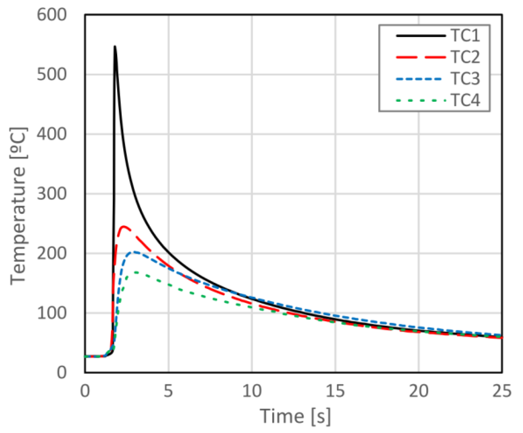
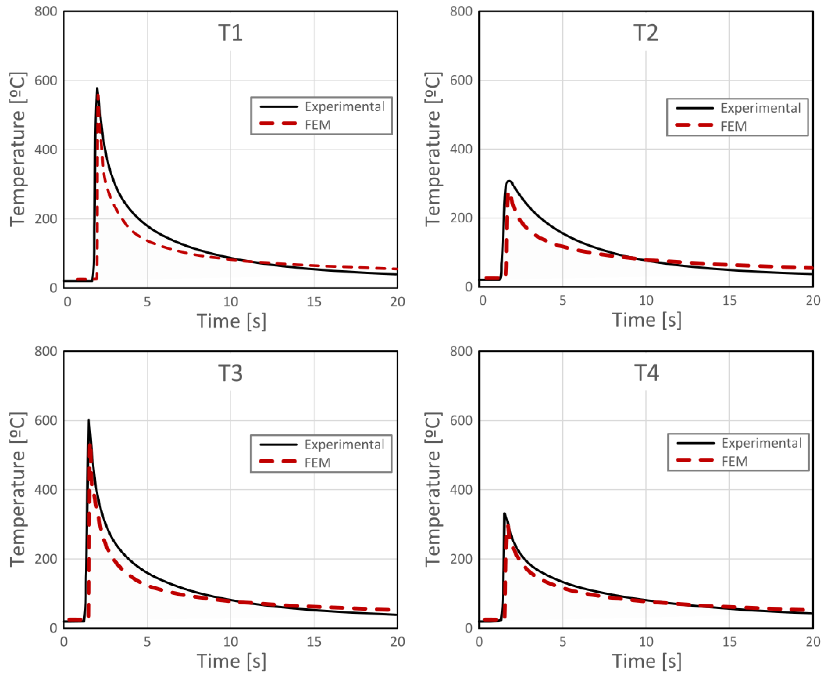
Figure 10 shows the comparison between the experimental evolution of temperatures (dotted black) and the temperatures predicted by the fitted FEM model (blue) in the same places. There is still some room for improvement in the maximum temperatures in thermocouples 3 and 4 and the temperature evolution in thermocouples 1 and 3, but the overall matching is good. The maximum temperature is mostly dependent on conical Gaussian parameters, while temperature evolution depends mainly on the convection coefficient, which has not been considered in this study.

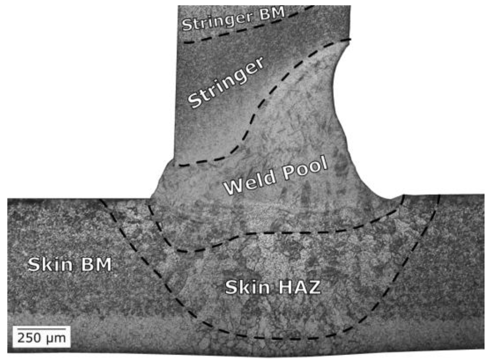
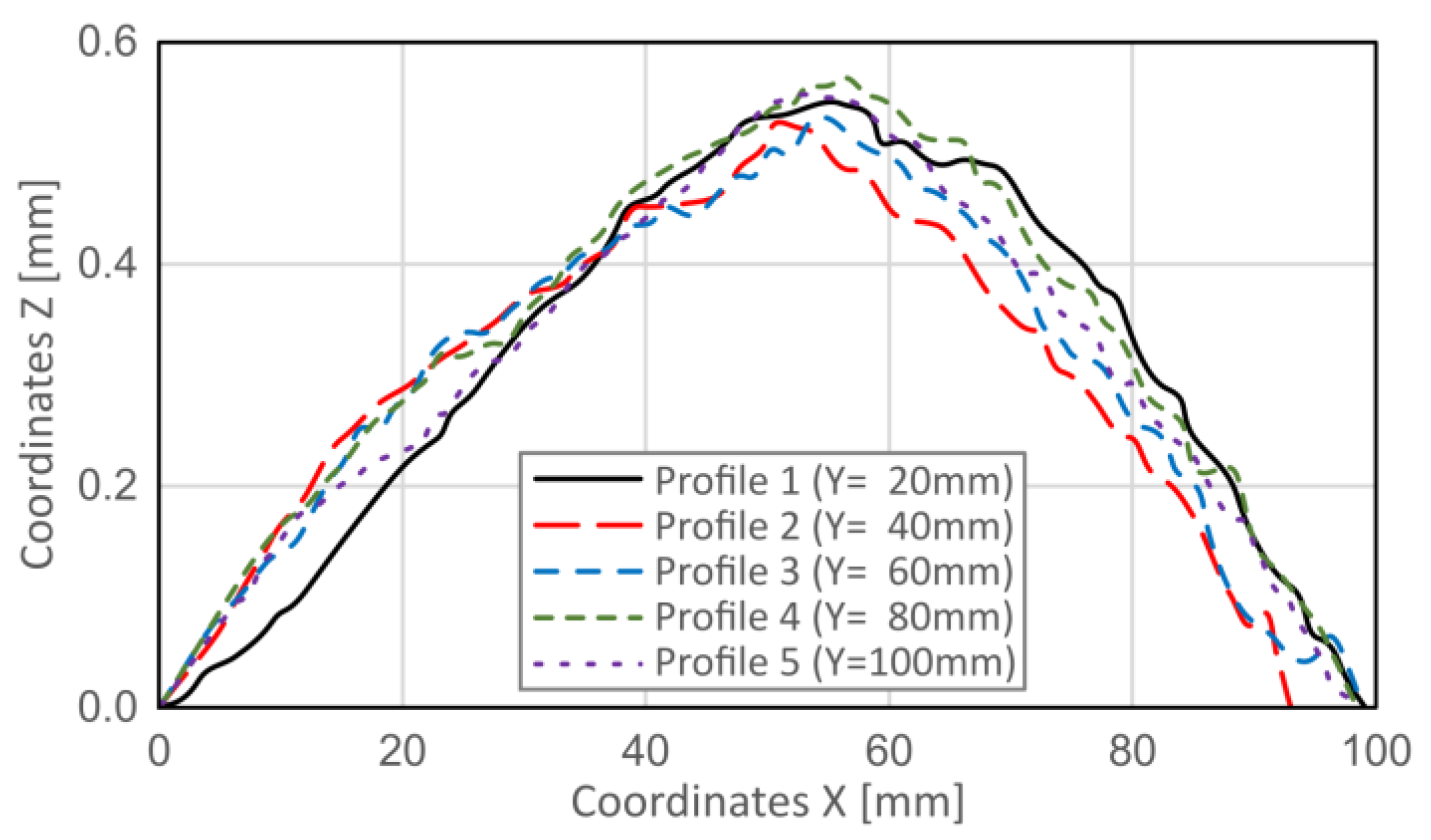
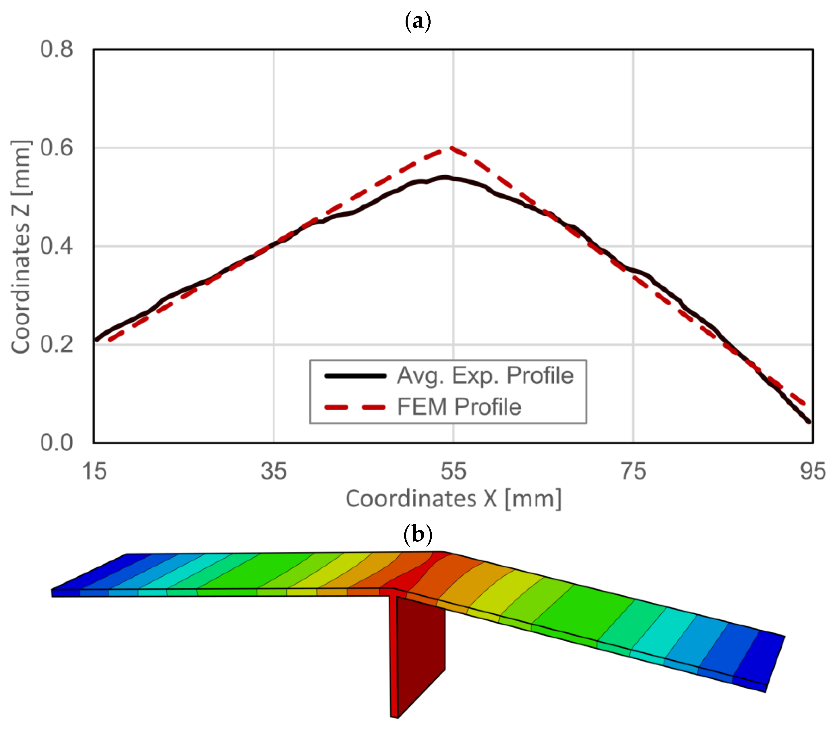
Figure 11a compares the average of the five profiles measured with the central profile of the fitted FEM model. The simulation results match the experimental data on the flanks but differ in the central area. The model cannot reproduce the round shape of the welded joint. In terms of angular distortion, the FEM model deformation is 1.31° while the specimen is 1.37°. Thus, the angular distortion error is 5.3%, which is considered highly satisfactory.

4. Conclusions

A methodology to find the best finite element Conical Gaussian heat flux parameters has been described and validated using experimental data from the dissimilar laser welding process. Its aim is the multi-objective fitting of titanium laser welding. The methodology can be summarized in five steps: implementation of a fractional factorial design, simulation of thermal and mechanical FEM models, creation of mathematical models, application of a response surface method to find the best unknown parameters, and the validation of results using experimental data. The result is an accurate FEM model that reproduces the temperatures and distortions of a Titanium welded joint.

Four heat flux parameters were studied: top radius re, lower radius ri, cone height yi, and process efficiency (η). FEM results show good agreement with experimental data. The best matching parameters for a Conical Gaussian heat flux are r_e = 0.41, r_i = 0.29, y_i = 0.78, and η = 0.5. The temperature average error is 8.2%, the angular distortion error is 5.3%, and the weld pool shape approximates the experimental macrograph. Based on the above results, new designs for experiments and simulations can be implemented to improve the accuracy of results. However, the authors consider that the obtained accuracy is highly satisfactory; thus, subsequent model improvements are not necessary in this case. The above parameters provide good results compared with experimental data in an affordable amount of time. Thermal models were simulated in just 24 h and mechanical models in 160 h. The implementation of this methodology avoids the classic trial and error process, which is a tedious job, does not assure good results, and takes an undetermined amount of time.

References

1. Belisle, M.J. Aerodynamic Design for Swept-wing Laminar Flow Internet. Ph.D. Thesis, Texas A & M University, College Station, TX, USA, 2013. Available online: https://oaktrust.library.tamu.edu/handle/1969.1/151655 (accessed on 30 June 2022).
2. Kashaev, N.; Ventzke, V.; Çam, G. Prospects of laser beam welding and friction stir welding processes for aluminum airframe structural applications. J. Manuf. Process. 2018, 36, 571–600. [Google Scholar] [CrossRef]
3. Gialos, A.A.; Zeimpekis, V.; Alexopoulos, N.D.; Kashaev, N.; Riekehr, S.; Karanika, A. Investigating the impact of sustainability in the production of aeronautical subscale components. J. Clean. Prod. 2018, 176, 785–799. [Google Scholar] [CrossRef]
4. Alexopoulos, N.D.; Gialos, A.A.; Zeimpekis, V.; Velonaki, Z.; Kashaev, N.; Riekehr, S.; Karanika, A. Laser beam welded structures for a regional aircraft: Weight, cost and carbon footprint savings. J. Manuf. Syst. 2016, 39, 38–52. [Google Scholar] [CrossRef]
5. Kannatey-Asibu, E., Jr. Principles of Laser Materials Processing Laser Welding; John Wiley & Sons, Inc.: Hoboken, NJ, USA, 2009. [Google Scholar]
6. Blackburn, J. Laser welding of metals for aerospace and other applications. In Welding and Joining of Aerospace Materials; Woodhead Publishing: Sawston, UK; pp. 75–108.
7. Lindgren, L.E.; Jonsson, M.; Karlsson, L.; Linden, G. Deformation and Stresses during Automatic Butt-Welding. In The Effects of fabrication Related Stresses on Product Manufacture and Performance. International Conference: 23/09/1985-25/09/1985; Welding Institute: Cambridge, UK, 1985; p. 285. [Google Scholar]
8. Colegrove, P.; Ikeagu, C.; Thistlethwaite, A.; Williams, S.; Nagy, T.; Suder, W.; Steuwer, A.; Pirling, T. Welding process impact on residual stress and distortion. Sci. Technol. Weld. Join. 2009, 14, 717–725. [Google Scholar] [CrossRef] [Green Version]
9. Biswas, P.; Mandal, N.R.; Das, S. Prediction of welding deformations of large stiffened panels using average plastic strain method. Sci. Technol. Weld. Join. 2011, 16, 227–231. [Google Scholar] [CrossRef]
10. Ueda, Y.; Fukuda, K.; Tanigawa, M. New measuring method of three dimensional residual stresses based on theory of inherent strain (welding mechanics, strength & design). Trans. JWRI 1979, 8, 249–256. [Google Scholar]
11. Hibbitt, H.D.; Marcal, P.V. A numerical, 14hermos-mechanical model for the welding and subsequent loading of a fabricated structure. Comput. Struct. 1973, 3, 1145–1174. [Google Scholar] [CrossRef]
12. Friedman, E. Thermomechanical Analysis of the Welding Process Using the Finite Element Method. J. Press. Vessel Technol. 1975, 97, 206–213. [Google Scholar] [CrossRef]
13. Oddy, A.S.; Goldak, J.A.; McDill, J.M.J. Transformation Plasticity and Residual Stresses in Single-Pass Repair Welds. J. Press. Vessel Technol. 1992, 114, 33–38. [Google Scholar] [CrossRef]
14. Lindgren, L.-E. Finite Element Modeling and Simulation of Welding. Part 1: Increased Complexity. J. Therm. Stress. 2001, 24, 141–192. [Google Scholar] [CrossRef]
15. Lindgren, L.-E. Finite Element Modeling and Simulation of Welding. Part 2: Improved Material Modeling. J. Therm. Stress. 2001, 24, 195–231. [Google Scholar] [CrossRef]
16. Lindgren, L.-E. Finite Element Modeling and Simulation of Welding. Part 3: Efficiency and Integration. J. Therm. Stress. 2001, 24, 305–334. [Google Scholar] [CrossRef]
17. He, X. Finite Element Analysis of Laser Welding: A State of Art Review. Mater. Manuf. Process. 2012, 27, 1354–1365. [Google Scholar] [CrossRef]
18. Zhu, X.; Chao, Y. Effects of temperature-dependent material properties on welding simulation. Comput. Struct. 2002, 80, 967–976. [Google Scholar] [CrossRef]
19. Rosenthal, D. Mathematical Theory of Heat Distribution during Welding and Cutting. Weld. J. 1941, 20, 220–234. [Google Scholar]
20. Rosenthal, D. The theory of moving sources of heat and its application to metal treatments. Trans. ASME 1946, 68, 849–866. [Google Scholar]
21. Pavelic, V.; Tanbakuchi, R.; Uyehara, O.A.; Myers, P.S. Experimental and Computed Temperature Histories in Gas Tungsten-Arc Welding of Thin Plates. Weld. J. 1969, 48, 295–305. [Google Scholar]
22. Goldak, J.; Chakravarti, A.; Bibby, M. A new finite element model for welding heat sources. Metall. Trans. B 1984, 15, 299–305. [Google Scholar] [CrossRef]
23. Aissani, M.; Guessasma, S.; Zitouni, A.; Hamzaoui, R.; Bassir, D.; Benkedda, Y. Three-dimensional simulation of 304L steel TIG welding process: Contribution of the thermal flux. Appl. Therm. Eng. 2015, 89, 822–832. [Google Scholar] [CrossRef]
24. Deng, D.; Murakawa, H. Numerical simulation of temperature field and residual stress in multi-pass welds in stainless steel pipe and comparison with experimental measurements. Comput. Mater. Sci. 2006, 37, 269–277. [Google Scholar] [CrossRef]
25. Gery, D.; Long, H.; Maropoulos, P. Effects of welding speed, energy input and heat source distribution on temperature variations in butt joint welding. J. Mater. Process. Technol. 2005, 167, 393–401. [Google Scholar] [CrossRef]
26. Podder, D.; Mandal, N.R.; Das, S. Heat source modeling and analysis of submerged arc welding. Weld. J. 2014, 93, 183–192. [Google Scholar]
27. Cîndea, L.; Haţiegan, C.; Pop, N.; Negrea, R.; Răduca, E.; Gillich, G.-R.; Dănuţ, M.; Nedeloni, M.-D. The influence of thermal field in the electric arc welding of X60 carbon steel components in the CO2 environment. Appl. Therm. Eng. 2016, 103, 1164–1175. [Google Scholar] [CrossRef]
28. Ahn, J. Experimental Characterisation and Numerical Simulation of Fibre Laser Welding of AA 2024-T3 and Ti-6Al-4V Internet; Imperial College: London, UK, 2016. [Google Scholar] [CrossRef]
29. Behúlová, M.; Babalová, E.; Nagy, M. Simulation model of Al-Ti dissimilar laser welding-brazing and its experimental verification. IOP Conf. Ser. Mater. Sci. Eng. 2017, 179, 012007. [Google Scholar] [CrossRef]
30. Chuan, L.; Jianxun, Z.; Jing, N. Numerical and Experimental Analysis of Residual Stresses in Full-Penetration Laser Beam Welding of Ti6Al4V Alloy. Rare Met. Mater. Eng. 2009, 38, 1317–1320. [Google Scholar] [CrossRef] [Green Version]
31. Mendizabal, A. A Computationally Efficient and Global Weld Modelling Strategy for Complex Structures. Master’s Dissertation, Mondragon Goi Eskola Politeknikoa, Mondragon, Spain, 2011. [Google Scholar]
32. Son, K.; Yang, Y.; Beom, H. Analysis of angular distortion in weldments using laminated plate theory. Sci. Technol. Weld. Join. 2000, 5, 245–249. [Google Scholar] [CrossRef]
33. Deng, D.; Murakawa, H.; Liang, W. Numerical simulation of welding distortion in large structures. Comput. Methods Appl. Mech. Eng. 2007, 196, 4613–4627. [Google Scholar] [CrossRef]
34. Fomin, F.; Froend, M.; Ventzke, V.; Alvarez, P.; Bauer, S.; Kashaev, N. Metallurgical aspects of joining commercially pure titanium to Ti-6Al-4V alloy in a T-joint configuration by laser beam welding. Int. J. Adv. Manuf. Technol. 2018, 97, 2019–2031. [Google Scholar] [CrossRef] [Green Version]
35. ASM4902E—Titanium Sheet, Strip, and Plate, Commercially-Pure, Annealed 40.0 ksi (276 Mpa) Yield Strength. ASM, 1986.
36. AMS4911F—Titanium Alloy, Sheet, Strip, and Plate, 6Al–4V, Annealed. ASM, 1988.
37. Froend, M.; Fomin, F.; Riekehr, S.; Alvarez, P.; Zubiri, F.; Bauer, S.; Klusemann, B.; Kashaev, N. Fiber laser welding of dissimilar titanium (Ti-6Al-4V/cp-Ti) T-joints and their laser forming process for aircraft application. Opt. Laser Technol. 2017, 96, 123–131. [Google Scholar] [CrossRef]
38. Dong, P. Residual stresses and distortions in welded structures: A perspective for engineering applications. Sci. Technol. Weld. Join. 2005, 10, 389–398. [Google Scholar] [CrossRef]
39. Argyris, J.H.; Vaz, L.E.; Willam, K.J. Integrated Finite-Element Analysis of Coupled Thermoviscoplastic Problems. J. Therm. Stress. 1981, 4, 121–153. [Google Scholar] [CrossRef]
40. Mahin, K.W.; Winters, W.; Holden, T.M.; Hosbons, R.R.; MacEwen, S.R. Prediction and measurement of residual elastic strain distributions in gas tungsten arc welds. Weld. J. 1991, 70, 245–260. [Google Scholar]
41. Smith, M. ABAQUS/Standard User’s Manual, Version 2016. Dassault Systèmes Simulia Corp: Providence, RI, USA, 2016. [Google Scholar]
42. JmatPro®. Sente Software Ltd.: Guildford, UK, 2016. Available online: https://www.sentesoftware.co.uk/jmatpro(accessed on 21 September 2022).
43. Titanium Properties. Institute for Energy Technology (IFE): Kjeller, Norway, 1985.
44. Selection of Technical Data Sheets. Pxprecimet: La Chaux-de-Fonds, France, 2012.
45. Adamus, K.; Kucharczyk, Z.; Wojsyk, K.; Kudla, K. Numerical analysis of electron beam welding of different grade titanium sheets. Comput. Mater. Sci. 2013, 77, 286–294. [Google Scholar] [CrossRef]
46. Escribano-García, R.; Lostado-Lorza, R.; Fernández-Martínez, R.; Villanueva-Roldán, P.; Mac Donald, B.J. Improvement in Manufacturing Welded Products through Multiple Response Surface Methodology and Data Mining Techniques. In International Joint Conference SOCO’14-CISIS’14-ICEUTE’14; Springer International Publishing: Cham, Switzerland, 2014; pp. 301–310. [Google Scholar]
47. Lorza, R.L.; García, R.E.; Calvo, M.Á.M.; Múgica-Vidal, R. Improvement in the Design of Welded Joints of EN 235JR Low Carbon Steel by Multiple Response Surface Methodology. Metals 2016, 6, 205. [Google Scholar] [CrossRef] [Green Version]
48. Islam, M.; Buijk, A.; Rais-Rohani, M.; Motoyama, K. Process parameter optimization of lap joint fillet weld based on FEM–RSM–GA integration technique. Adv. Eng. Softw. 2015, 79, 127–136. [Google Scholar] [CrossRef]
49. Myers, R.H.; Montgomery, D.C.; Anderson-Cook, C.M. Response Surface Methodology; Allyn and Bacon, Inc.: Boston, MA, USA, 1971. [Google Scholar]
50. Box, G.E.P.; Behnken, D.W. Some new three level designs for the study of quantitative variables. Technometrics 1960, 2, 455–475. [Google Scholar] [CrossRef]
51. Harrington, E.C. The Desirability Function. Ind Qual Control. 1965, 494–498. [Google Scholar]
52. R Core Team. R: A Language and Environment for Statistical Computing, Version 3.3.3; R Core Team: Vienna, Austria, 2017. Available online: www.R-project.org(accessed on 26 March 2017).
53. Wilkinson, L.; Dallal, G.E. Tests of Significance in Forward Selection Regression with an F-to-Enter Stopping Rule. Technometrics 1981, 23, 377–380. [Google Scholar]
54. Kuhn, M. Desirability: Function Optimization and Ranking via Desirability Functions. 2016. [Google Scholar]
55. Bertsekas, D.P. Nonlinear Programming. Edición: 2; Athena Scientific: Belmont, MA, USA, 1999. [Google Scholar]
Figure 1. Conical Gaussian heat flux model.
Jmmp 06 00130 g001
Figure 2. Welded sample: (a) Photo of the specimen with the thermocouples during welding and (b) Sketch of the T-joint with location of thermocouples.
Jmmp 06 00130 g002
Figure 3. Experimental temperature records during welding.
Jmmp 06 00130 g003
Figure 4. Micrograph showing molten weld pool and HAZ.
Jmmp 06 00130 g004
Figure 5. Angular distortions measurement.
Jmmp 06 00130 g005
Figure 6. Distortion of five profiles after welding.
Jmmp 06 00130 g006
Figure 7. FEM-model dimensions in mm and boundary conditions.
Jmmp 06 00130 g007
Figure 8. Thermo-mechanical properties of Titanium grades 2 and 5.
Jmmp 06 00130 g008
Figure 9. Correlations between inputs and outputs.
Jmmp 06 00130 g009
Figure 10. Temperature evolutions of the optimum case.
Jmmp 06 00130 g010
Figure 11. Distortions of the optimum case after welding: (a) Experimental comparison and (b) FEM vertical displacements.
Jmmp 06 00130 g011