Article

Multi-Level Hazard Detection Using a UAV-Mounted Multi-Sensor for Levee Inspection

1
School of Geodesy and Geomatics, Wuhan University, Wuhan 430079, China
2
Hubei Luojia Laboratory, Wuhan 430079, China
3
Wuhan RGSpace Co., Ltd., Wuhan 430073, China
4
National Institute of Natural Hazards, Ministry of Emergency Management of the People’s Republic of China, Beijing 100085, China
5
Key Laboratory of Compound and Chained Natural Hazards Dynamics, Beijing 100085, China
*
Authors to whom correspondence should be addressed.
Drones 2024, 8(3), 90; https://doi.org/10.3390/drones8030090
Submission received: 9 January 2024 / Revised: 16 February 2024 / Accepted: 19 February 2024 / Published: 6 March 2024

Abstract

:
This paper introduces a developed multi-sensor integrated system comprising a thermal infrared camera, an RGB camera, and a LiDAR sensor, mounted on a lightweight unmanned aerial vehicle (UAV). This system is applied to the inspection tasks of levee engineering, enabling the real-time, rapid, all-day, all-round, and non-contact acquisition of multi-source data for levee structures and their surrounding environments. Our aim is to address the inefficiencies, high costs, limited data diversity, and potential safety hazards associated with traditional methods, particularly concerning the structural safety of dam bodies. In the preprocessing stage of multi-source data, techniques such as thermal infrared data enhancement and multi-source data alignment are employed to enhance data quality and consistency. Subsequently, a multi-level approach to detecting and screening suspected risk areas is implemented, facilitating the rapid localization of potential hazard zones and assisting in assessing the urgency of addressing these concerns. The reliability of the developed multi-sensor equipment and the multi-level suspected hazard detection algorithm is validated through on-site levee engineering inspections conducted during flood disasters. The application reliably detects and locates suspected hazards, significantly reducing the time and resource costs associated with levee inspections. Moreover, it mitigates safety risks for personnel engaged in levee inspections. Therefore, this method provides reliable data support and technical services for levee inspection, hazard identification, flood control, and disaster reduction.

1. Introduction

Levee engineering serves as a crucial project to safeguard residents and agricultural production from the devastating impacts of flooding [1,2]. With the onset of increased rainfall during the flood season, the combined effects of floods and precipitation create substantial pressure differentials between the upstream and downstream slopes of levee structures. This often results in water easily backflowing through drainage pipes. Suppose there is a permeable layer within the levee engineering, this can lead to seepage, and the erosive effects of seepage may cause the loss of soil particles within the dam, forming weak spots and eventually resulting in piping. Water hazards such as backflow, seepage, and piping [3,4,5] may even lead to breaches and failures within the levee dam, posing severe threats to human life and property. Consequently, monitoring levee hazards [6,7] in water bodies such as rivers and lakes becomes a critical task during the annual flood control and disaster prevention period.
The environment surrounding levee engineering is complex, and patrol personnel find it challenging to promptly identify potential risks, such as minor cracks and seepage, during inspections, leading to low inspection efficiency. Particularly when encountering floods or exceptional circumstances, there is a need to increase the intensity and frequency of levee patrols and inspections, significantly heightening the safety risks for patrol personnel.
To overcome these challenges, we devised a multi-sensor system, integrating an RGB camera, a thermal infrared camera, and LiDAR (as illustrated in Figure 1). This advanced system is built upon a drone platform with a positioning and orientation system (POS) [8]. The RGB camera [9] delivers high-resolution RGB images, enabling patrol personnel to capture detailed visual information for visual interpretation. The LiDAR [10] provides precise three-dimensional point cloud data with spatial information, facilitating the quantification of surface morphology and structural features. Additionally, the thermal infrared camera [11] detects the thermal distribution of objects, uncovering potential areas with significant temperature variations. Simultaneously, we developed a set of preprocessing methods for multi-source data and a multi-level algorithm for detecting suspected hazardous situations.
In the algorithm development, our core idea was that levee engineering hazards generally involve seepage and water infiltration phenomena [12], with the flowing water temperature usually lower than that of other materials. Based on this concept, we initially used an improved dense nested attention network (DNA-Net) [13] to detect low-temperature regions in contrast-enhanced thermal infrared images. During the experimental process, we found that only image target detection typically identifies low-temperature targets such as individual trees, small clusters of vegetation, flowing water, and mixed areas of these features.
As is well known, the echo intensity of point clouds in pure water areas [14] is almost zero. Although the water in hazardous situations may contain sediment, aquatic plants, or other things, the overall echo intensity of the point cloud in this area remains low. Moreover, the lower the echo intensity of the point cloud within the detected area, the higher the water content. By combining the detection of low-temperature regions in thermal infrared images with the echo intensity information of point clouds, we can screen and quickly locate suspected hazard areas. Additionally, we can use the echo intensity of point clouds within the mask area to assist in determining the degree of danger in suspected hazard areas, facilitating the arrangement of regional inspection tasks. Furthermore, by projecting suspected hazard areas onto RGB images, patrol personnel can conduct visual interpretations based on the surrounding environment, further reducing their workload.
Based on these principles, this paper aims to develop a multi-sensor integrated drone system suitable for levee inspection and a relatively comprehensive multi-level hazard detection algorithm process. The contributions of this paper are listed as follows:
(1)
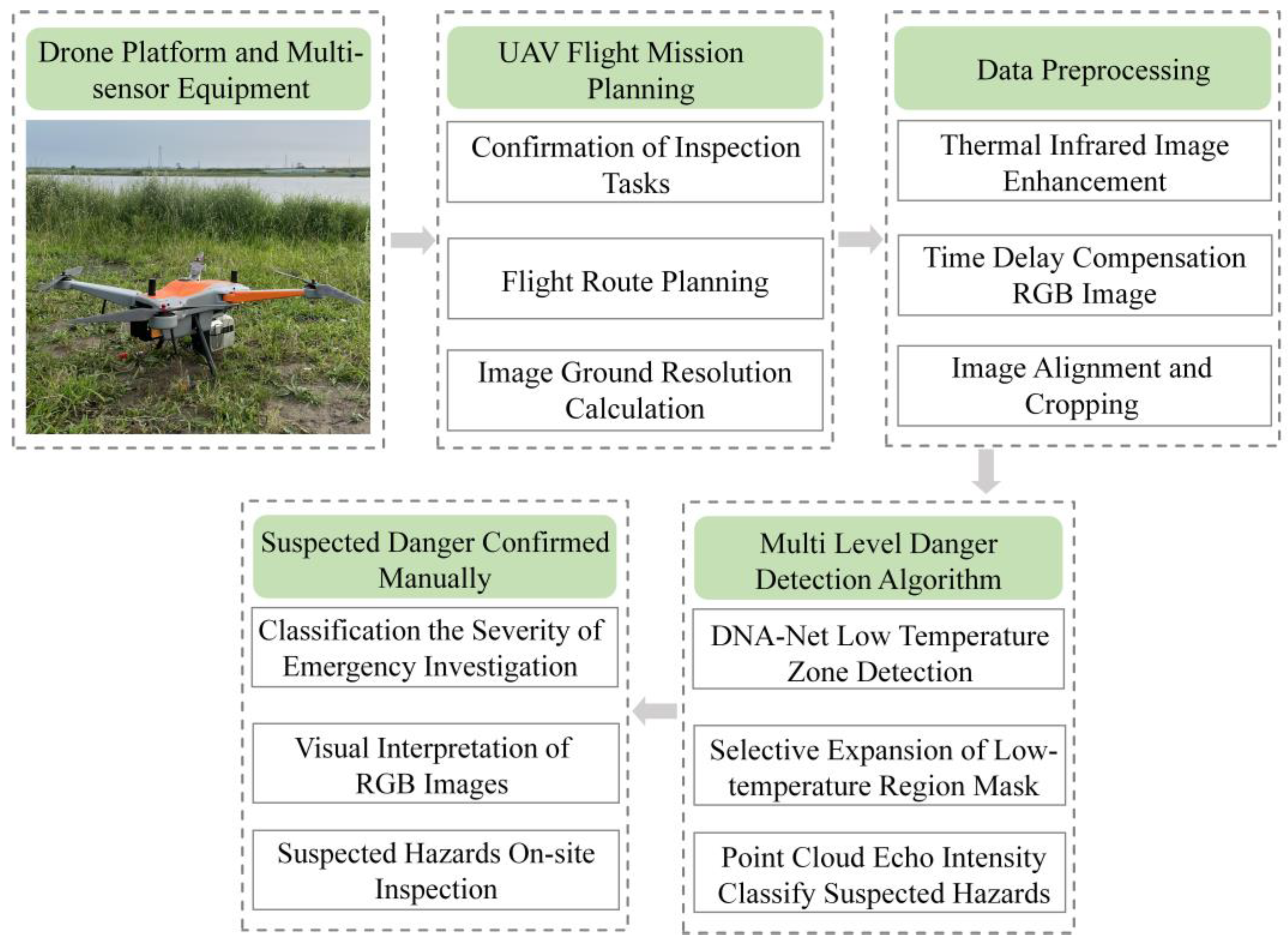
We developed a multi-sensor integrated drone system tailored towards levee engineering hazard inspection. On the basis of multi-sensor time synchronization, external parameter calibration between RGB and thermal infrared cameras is achieved, ultimately unifying multi-source data within the same spatiotemporal framework. Additionally, the temperature resolution capability of the thermal infrared camera at various drone flight altitudes was examined to ensure the effectiveness of data collection.
(2)
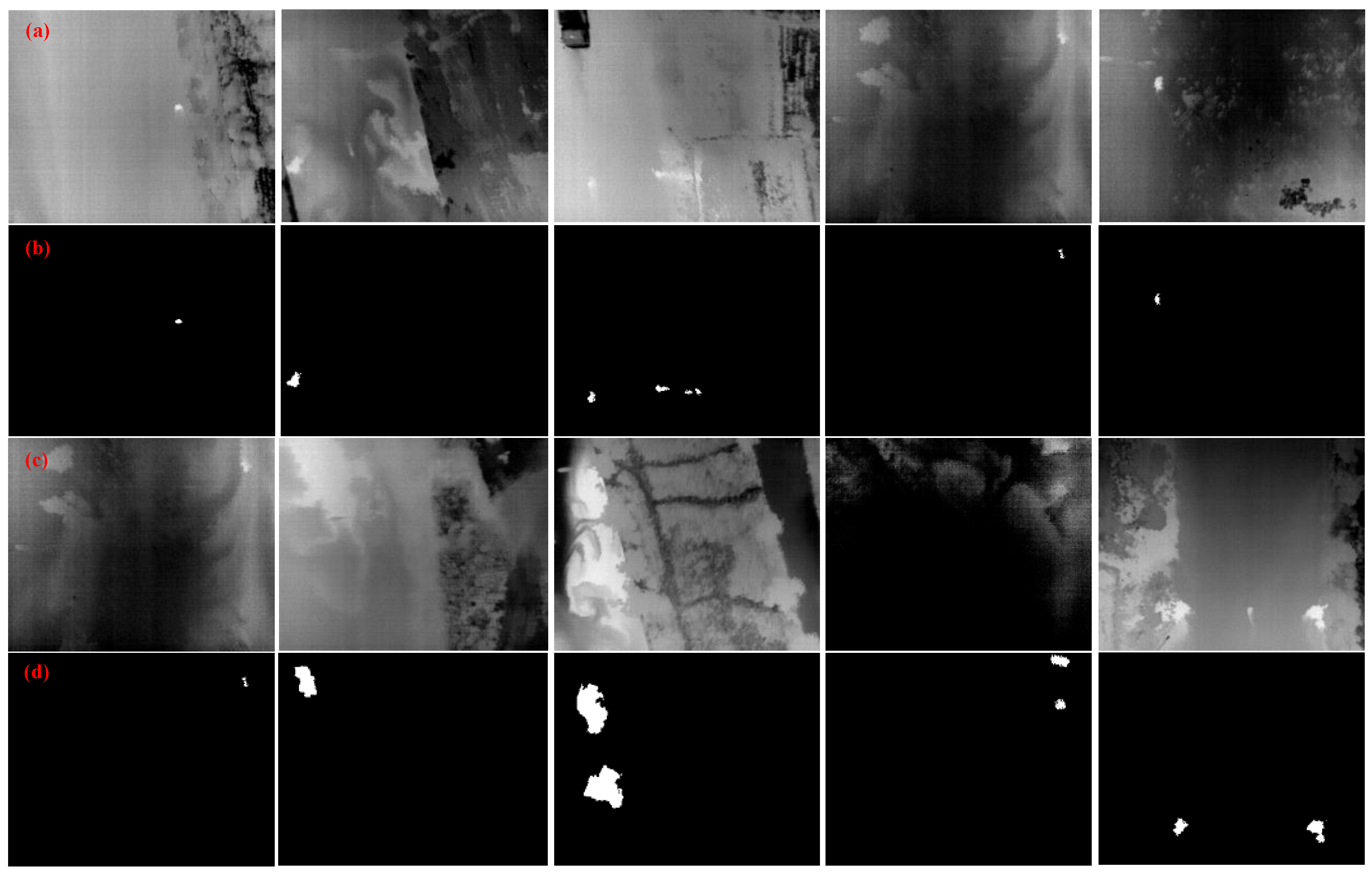
We annotated and constructed a dataset containing 739 sets of low-temperature targets in thermal infrared images, and applied the trained network to detect low-temperature areas in thermal infrared images. Subsequently, the echo intensity of the LiDAR point cloud data was used to differentiate between water bodies, and assess the potential danger level of suspected hazards. Finally, a visual interpretation of the suspected hazard areas was conducted using RGB images, further enhancing operational efficiency.
(3)
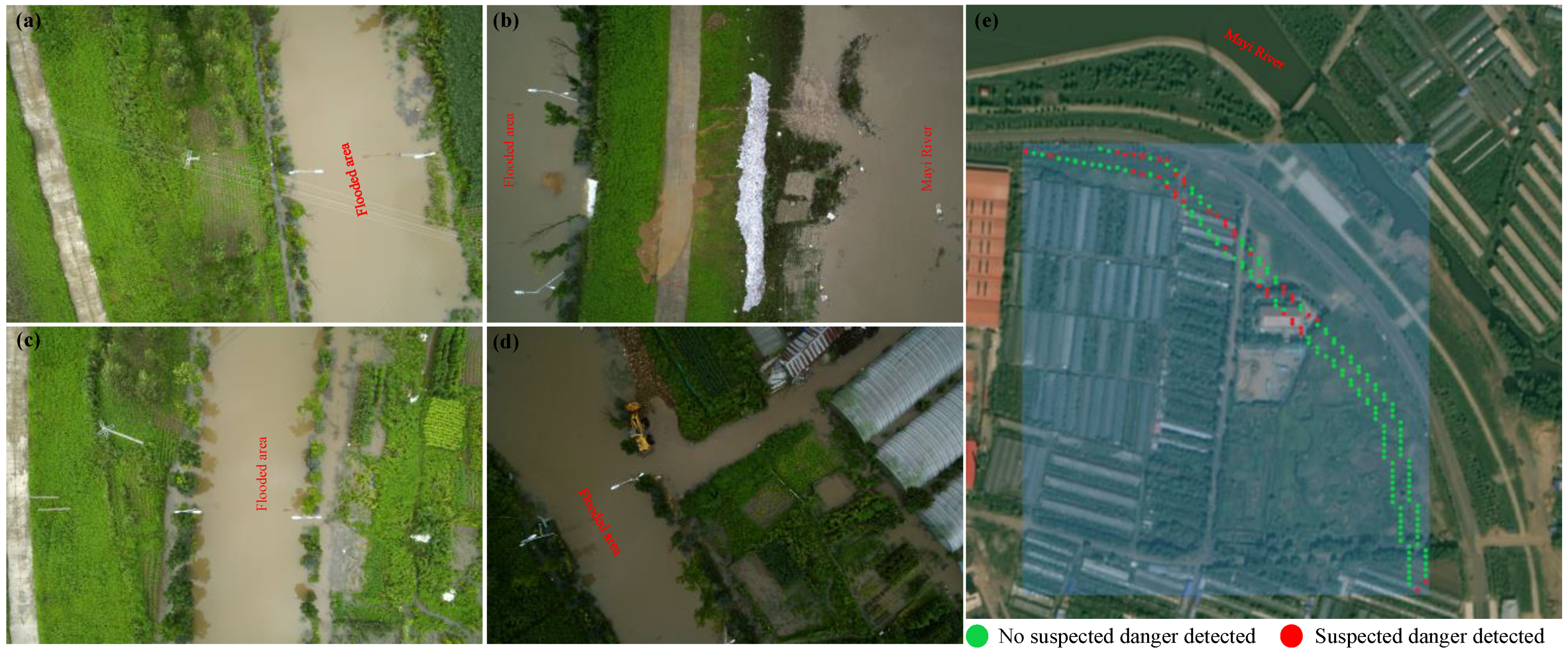
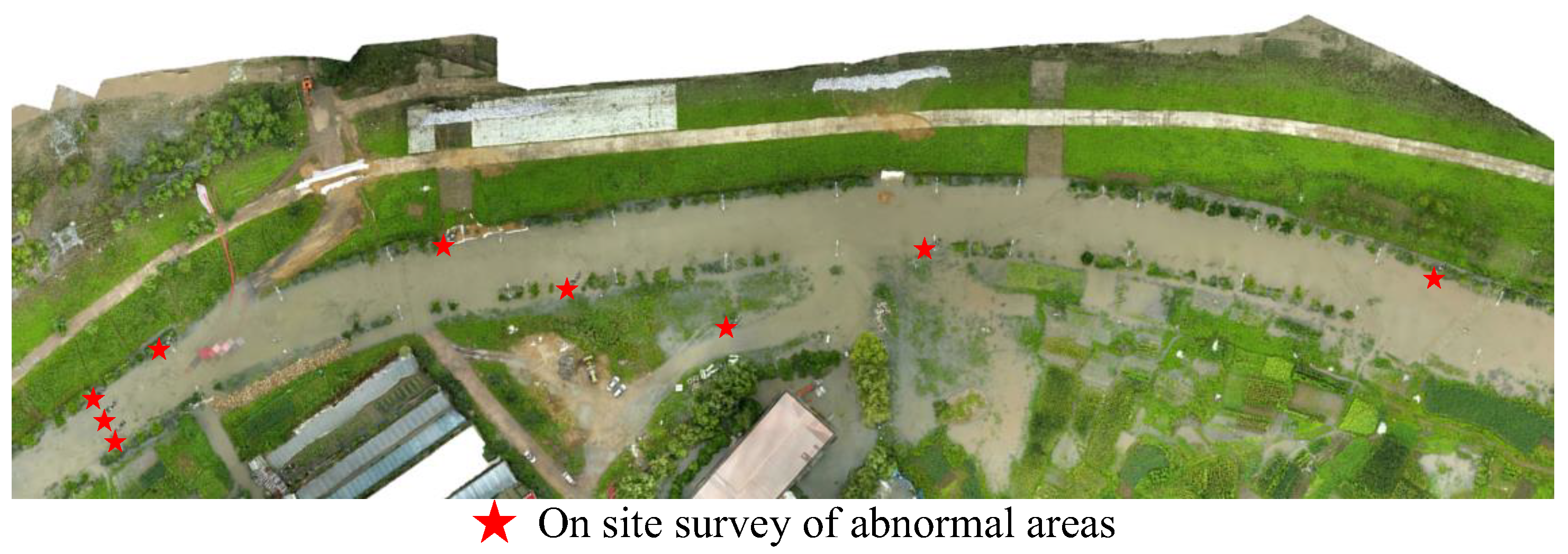
We applied the multi-sensor integrated drone system and the multi-level suspected hazard detection algorithm in the field during heavy rain in Heilongjiang Province, China. We tested the applicability of the equipment and the effectiveness of multi-level detection methods at the disaster site. Practice has proven that the approach can provide robust support for the prevention and handling of potential hazards and risks.

2. Related Levee Monitoring Methods

The monitoring methods used for levee hazards mainly include piezometers, seepage pressure gauges, electrical resistivity tomography, isotope tracing, temperature tracing, distributed fiber-optic temperature sensing, ground-penetrating radar systems, and hyperspectral imaging devices [15,16,17]. Piezometers are a traditional method for monitoring seepage; they measure the height of the water column in the tube to indicate the magnitude of the pore water pressure, detecting parameters such as dam seepage pressure, groundwater level, and seepage around the dam. Piezometers have a simple structure, are easy to manufacture and install, and are cost effective. However, they are prone to human-induced damage, pipe clogging, and long-term monitoring is time-consuming and labor-intensive, leading to potential errors and an information lag between measured data and actual conditions. Seepage pressure gauges measure internal pore water pressure or seepage pressure within structures. They feature high sensitivity, precision, and stability, are capable of signal transmission over long distances without distortion, have strong interference resistance, and are suitable for long-term observations.
Electrical resistivity tomography involves the penetration of liquids through anti-seepage layers, increasing the dielectric constant or decreasing the resistivity of the anti-seepage layer. Changes in capacitance and resistivity enable the monitoring of dam seepage conditions. Isotope tracing involves introducing appropriate isotopic tracers into the upstream area of the leakage section. Continuous monitoring of the tracers downstream, combined with hydrogeological material, allows for determining permeability coefficients and identifying seepage speed and direction. Temperature tracking entails burying susceptible temperature sensors at various depths within the dam. Seepage water affects the surrounding temperature field, and after the dissipation of temperature disturbances, fixed-point temperatures are measured. Distributed fiber-optic temperature measurement technology involves embedding optical cables inside the dam to achieve real-time temperature collection at various continuous measurement points along the dam. It allows for the spatial positioning of measurement points. However, these methods require instruments to be embedded within the dam, demanding careful construction to avoid structural damage and induce new seepage. Maintenance and replacement are challenging if the instruments are damaged and lack flexibility.
Ground-penetrating radar systems [18] utilize antennas to emit high-frequency electromagnetic waves toward the tested dam. Recording the reflected waves through pulse signals helps to detect internal features such as cracks and voids. However, the detection resolution of ground-penetrating radar decreases with detection depth, and other noise signals severely interfere with the quality of the reflected signals. Hyperspectral imaging devices [19] can obtain ultra-high-resolution hyperspectral images [20] with outstanding material identification capabilities. They can be used to monitor seepage locations based on the backscatter characteristics of water-permeated areas. However, the volume of data sharply rises with the increasing number of bands, and a high level of correlation between adjacent bands leads to information redundancy. Although satellite remote sensing can offer extensive data monitoring, its monitoring area and range cannot be adjusted in real-time. Additionally, satellite remote sensing has a relatively lower image resolution, making it challenging to capture surface details, and is more suitable for post-disaster analysis.

3. Materials and Methods

Due to the lack of adequate, reliable, and flexible monitoring technologies for levee engineering, manual network patrols are still necessary in the face of severe flood control situations [21]. Here, we develop multi-sensor equipment for levee inspection and hazard identification based on a light and compact UAV platform [22]. This equipment can collect diverse data in areas personnel may find inaccessible. Then, we propose a multi-source data-based, multi-level algorithm for detecting potential hazards. The algorithm can identify threats that are not readily observable by the human eye, thereby improving operational efficiency and ensuring the personal safety of levee inspection personnel. The framework is illustrated in Figure 2.

3.1. Sensors

The equipment consists of a Global Navigation Satellite System (GNSS) [23] positioning and orientation system, a LiDAR system, and the FLIR VUE Pro R thermal infrared camera [24]. This configuration can acquire high-precision, high-frequency position and orientation data, three-dimensional LiDAR data, high-resolution RGB, and thermal infrared images. Additionally, the LiDAR system and thermal infrared camera ensure that the equipment can operate around the clock, facilitating day and night inspections.
According to Planck’s law [25], any object with a temperature above absolute zero emits electromagnetic waves, including infrared radiation. The use of long-wave infrared (7.5–14 μm), with solid penetration capabilities [26], allows for the observation of ground objects through weather conditions such as clouds, haze, rain, and snow. Infrared cameras use photosensitive components to detect the infrared radiation emitted by objects. Through technologies such as photoelectric conversion and signal processing, these thermal radiation signals are converted into electrical signals. Further processing and calculation can transform electrical signals into visual grayscale images. Additionally, the higher the temperature of an object, the stronger the electromagnetic wave signals it emits. If there is a temperature difference between the detected target and the background, the energy difference in radiation manifests as the edge contours of the detected target in the infrared image. The FLIR Vue Pro R is a thermal imaging camera designed explicitly for small UAVs. It can capture precise non-contact temperature measurements and embed calibrated temperature data into each pixel. The technical specifications of the FLIR Vue Pro R camera are detailed in Table 1.
LiDAR measures the distance from the target to the LiDAR receiver by emitting a laser beam, obtaining accurate three-dimensional point cloud data. LiDAR-collected point cloud data has high precision and good anti-interference ability, is unaffected by changes in lighting conditions, and provides accurate spatial information. We selected the CHC Navigation AlphaAir 450 pocket LiDAR [27] based on its lightweight and highly integrated design concept. With a built-in camera, the entire payload weighs only 950 g, enabling high-precision, high-density, and efficient real-time data acquisition. LiDAR technical specifications are detailed in Table 2.
The RGB camera captures visible light reflected from the surface of an object during the imaging process, influenced by both the object’s reflectivity and external lighting intensity. Under sufficient illumination, the imaging quality is higher, containing richer information, complete texture details, and more pronounced structural features. In overcast or nighttime conditions, when the lighting intensity decreases, imaging quality significantly deteriorates. However, the image information is acceptable, and it requires lower professional expertise for levee patrol personnel, serving as an auxiliary judgment basis. Utilizing the built-in 24-megapixel camera in the AlphaAir 450 LiDAR system, it can generate a digital orthophoto map (DOM), digital surface model (DSM) [28], and colorized point clouds. The technical parameters of the RGB camera are detailed in Table 3.
The multi-sensor integrated equipment we developed is an independent system that can be mounted on a drone platform. In this study, it is deployed on the CHC Navigation BB4 mini UAV [29] platform, providing a flight endurance of 50 min. The technical specifications of the BB4 mini UAV platform are outlined in Table 4.

3.2. Multi-Sensor Integrated Equipment Based on UAV Platform

3.2.1. Time Synchronization

The unified time baseline requires ensuring that the absolute time accuracy of the acquisition system is within a specific error range [30] and is capable of achieving ultra-low-latency synchronous data collection for multiple sensors. In the AA450 system, the synchronization method for the LiDAR and RGB camera is hard synchronization [31]. Due to the different triggering mechanisms of the thermal infrared camera compared to regular RGB camera, the synchronization between the thermal infrared camera and the AlphaAir 450 LiDAR system through soft synchronization. Soft synchronization may result in a lack of strict synchronization between the trigger times of the thermal infrared camera and the AlphaAir 450 LiDAR system. Therefore, additional data preprocessing steps are required to align the images.
In the AlphaAir 450 LiDAR system, the GNSS data, LiDAR data, and RGB camera images can be processed and packaged in real time. To ensure the synchronization accuracy and real-time requirements of the data, the system’s core processor is the STM32MP157. This processor includes a dual-core Cortex-A7 and a Cortex-M4. The application on the Cortex-M4 core uses an interrupt-driven approach to receive data from the inertial navigation system, GPS module, and camera feedback signals. This ensures the accuracy of the time tagging. The Linux system runs on the Cortex-A7 core, providing data packaging, compression, and unified storage functions. External communication relies on interface programs within the Linux system. Communication and data exchange between the Cortex-A7 and Cortex-M4 occurs through an internal high-speed bus which minimizes data latency. The GNSS module sends a PPS (pulse per second) signal every second, followed by the output of time and location data through a data interface. The Cortex-M4 core collects and processes these data. Approximately 10 ms after each PPS signal, the GNSS module sends the time and location information via serial communication. The CPU captures this trigger signal, receiving data from the module. The camera generates a feedback signal when taking a photo. The Cortex-M4 core records when this signal occurs, similar to the inertial navigation system synchronization signal, and attaches a time tag. The data are then packaged and sent to the Cortex-A7 core for further processing.

3.2.2. Spatial Reference Standardization

Due to the maturity and widespread application of the AlphaAir 450 LiDAR system, we did not conduct a separate extrinsic calibration for the camera–LiDAR system when unifying the spatial reference. We devised a multi-sensor system by rigidly affixing the FLIR Vue Pro R thermal infrared camera to the AlphaAir 450 device. Consequently, our primary focus in this section is on addressing the extrinsic calibration between the thermal infrared camera [32] and the AlphaAir 450 LiDAR system.
Based on the relationship between focal length f , flight height H , pixel size a , and ground sample distance (GSD), as defined by Formula (1), the actual ground size represented by the pixels in thermal infrared and RGB images can be determined.
G S D = ( H × a ) / f
Due to the lower GSD of thermal infrared images, we initially employ a downsampling approach on RGB images to reduce spatial disparities between the two types of images. Subsequently, a feature point extraction algorithm is utilized to extract corresponding points for matching, ultimately solving for the extrinsic matrix between the RGB camera and the thermal infrared camera. However, thermal infrared images capture radiation information from the terrain, while RGB images reflect information related to surface reflection. Due to differences in imaging mechanisms, thermal infrared and RGB images exhibit significant variations in texture, grayscale characteristics, and resolution. Traditional feature extraction methods often rely on pixel grayscale gradients for feature point detection. However, the instability of single-pixel grayscale and gradients between infrared and RGB images can lead to feature matching errors or failures. Given the lower resolution of thermal infrared images, our strategy involves the use of the Superpoint [33] network to extract as many feature points as possible. In the feature matching stage, a multi-level feature matching approach is employed to ensure the robustness of feature descriptors, thereby enhancing the effective matching between thermal infrared and RGB images.
Superpoint has proposed a self-supervised framework comprising two networks: the base detector and superpoint. The base detector detects corner points as candidate feature points, while superpoint outputs feature points and descriptors. A synthetic dataset is created using three-dimensional objects to train the network and enhance its ability to extract corner points. Subsequently, the pre-trained network is applied to extract corner points from the publicly available MS-COCO dataset. Simultaneously, the original photos in the dataset are subjected to rotation and scaling to generate new image data, followed by another round of corner point extraction to ensure the network’s generalization capability. Through empirical validation, the authors have demonstrated that Superpoint can repeatedly detect interest points that are more diverse compared to other traditional corner point detection methods.
In the feature-matching stage, assuming the set of feature points extracted from the thermal infrared image is X = ( x 1 , , x m ) , and the collection of feature points extracted from the RGB image is Y = ( y 1 , , y n ) , we select a feature point x m from the feature point set X . Based on the descriptor, we calculate the Euclidean distance from point x m to all feature points in a set Y . The closest point is denoted as y n 1 , and the distance between their descriptors is indicated as d n 1 . The second closest neighbor and the distance between their descriptors are represented as y n 2 and d n 2 , respectively. The ratio of the distance between the nearest and second nearest neighbors, denoted as r , is given by r = d n 1 / d n 2 . When r 1 , a smaller value of r corresponds to a more minor matching error. The initial matching process is considered complete when r is less than the predefined threshold.
According to the a priori knowledge of the consistent slope of lines connecting nearby matching points in two images, the initial set of matching points is constrained. Matches with slopes exceeding a threshold are considered as erroneous matches, further improving matching accuracy. Suppose a pair of matching points in thermal infrared and RGB images have coordinates X ( x R G B , y R G B ) and Y ( x T I R , y T I R ) , the slope of the line connecting these two points is calculated as follows:
θ = a r c t a n y R G B y T I R x R G B x T I R
Next, RANSAC [34] is employed to identify the optimal transformation matrix, eliminate outliers, and obtain the final set of matching points denoted as F = { ( X m , Y m ) } m = 1 M ; M represent the total number of matching points obtained in the end.

3.2.3. Thermal Infrared Camera Temperature Resolution

A thermal infrared camera responds to the total infrared energy detected by the sensor, with the majority of infrared energy coming from objects and only a minimal amount from the camera itself. However, throughout the imaging process, it is not possible to completely eliminate the impact of the surrounding materials on the detector and optical path. The FLIR VUE PRO R camera has a measurement accuracy of ±5 °C. Without compensation for ambient temperature, changes in the camera body or lens temperature can significantly alter the temperature readings provided by the thermal imager. The official recommendation for achieving ambient temperature compensation is to measure the temperatures of the thermal imager and optical path from up to three different positions. Due to factors such as atmospheric absorption and emissivity, an increase in observation distance introduces uncertainties in the measurement values. The official documentation indicates that the current error calculation values generally apply to laboratory or outdoor short-range scenarios (within 20 m).
During levee inspection missions conducted using drones and multi-sensor equipment, the first step involves planning flight routes based on on-site conditions. Potential flight obstacles such as power lines, trees, and signal towers may arise within the monitoring range, necessitating an adaptable approach to setting the flight altitude. Therefore, consideration must be given to the impact of flight altitude on the sensitivity of the thermal imager. In our mission, the ability of the thermal imager to discern surface temperatures is crucial. To validate the accuracy of the thermal imaging camera data and assess the influence of flight altitude on the thermal resolution, we arranged water bodies of varying temperatures, shapes, and sizes on the ground. Temperature measurements were conducted using a thermometer before and after takeoff, and thermal infrared images obtained at different altitudes were analyzed. This process ensures that the selected thermal infrared camera’s temperature resolution can effectively observe low-temperature targets within the dam inspection mission area. All FLIR thermal imagers are calibrated according to factory parameters during production. However, electronic components may age over time, leading to calibration drift and inaccurate temperature measurements. To ensure the accuracy of the thermal imager, it is recommended to perform regular calibration at the manufacturer’s facility, with an annual calibration being suggested by the official guidelines.

3.3. Data Preprocessing

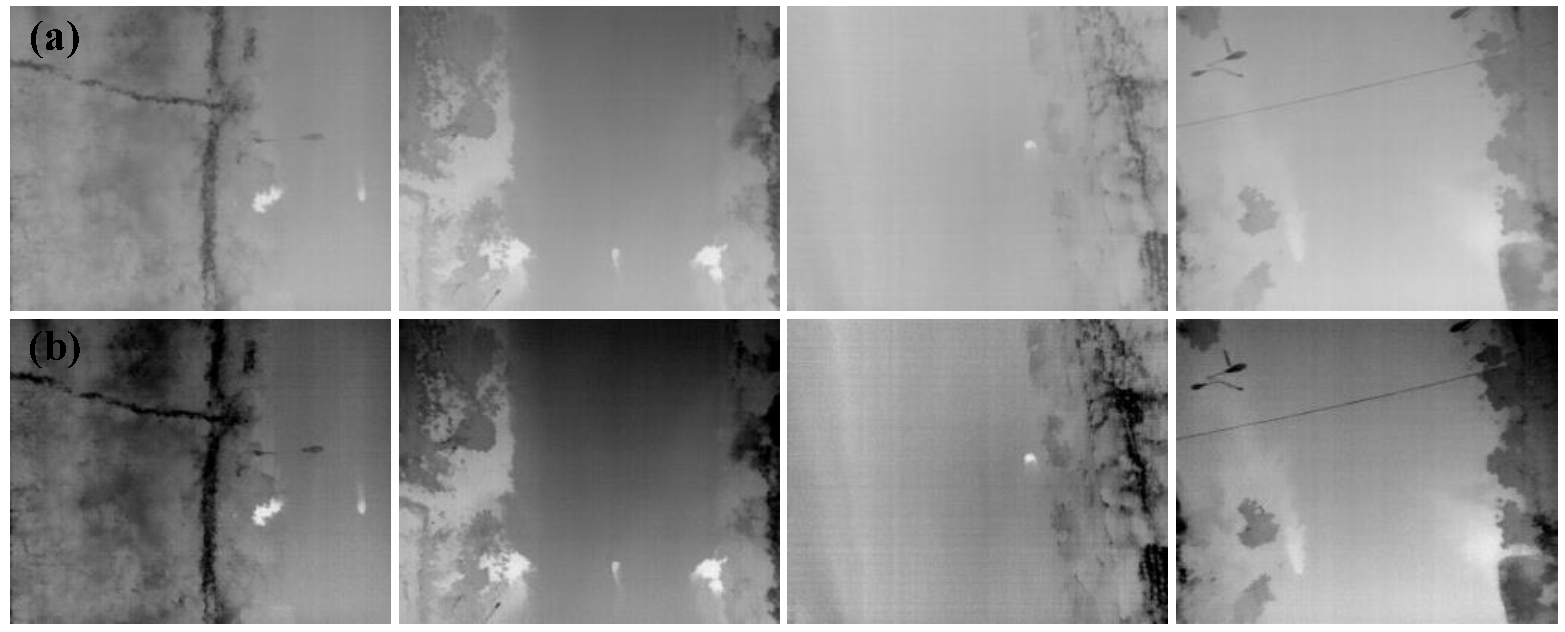
3.3.1. Infrared Image Enhancement

The original thermal infrared images we acquire typically exhibit lower grayscale values for objects with lower temperatures, transitioning towards darker shades. In the preprocessing stage, to facilitate the production of datasets and subsequent target detection algorithms, we initially perform an inverse transformation on all thermal infrared image pixels. Specifically, we subtract each pixel’s grayscale value from 255, resulting in objects with lower temperatures appearing brighter with higher grayscale values, transitioning towards white.
Due to the characteristics of the thermal infrared camera’s detection components and variations in the distribution of surface temperatures, the thermal infrared images exhibit noticeable grayscale changes only when there is a significant variation in ground temperatures. As a result, the contrast in the obtained thermal infrared images is generally low, and the edges of the targets may not be sufficiently sharp. Additionally, the rapid movement of the UAV can exacerbate the blurring of thermal infrared images. Nevertheless, we aim to utilize the contours and grayscale gradients formed by surface temperature distribution variances to initially screen for potential hazard areas through target detection. Therefore, in the data preprocessing stage, we opt to enhance the thermal infrared image through contrast stretching [35]. The objective is to improve the contrast between the background and targets, thereby enhancing the detection efficiency and accuracy of potential hazards in levee engineering. We employ contrast stretching to enhance the image, extending the grayscale values across the 0–255 range. The stretched pixel values can be calculated by the following formula:
I ( x , y ) s t r e t c h e d = ( I ( x , y ) I m i n ) × 255 I m a x I m i n

3.3.2. Alignment of Thermal Infrared, RGB and Point Cloud Images

In Section 3.2.2, we computed the relative position relationship matrix between the RGB and thermal infrared cameras, achieving a rough alignment. However, in practice, the long-wave infrared camera requires non-uniformity correction (NUC) during operation to reduce errors [36]. NUC will periodically pause the camera operation, delaying the time between the thermal infrared camera and the RGB camera during aerial missions. Consequently, when the thermal infrared and RGB cameras execute tasks in the air, achieving complete time synchronization is impossible.
In our system, we record the capture time of the RGB camera and the trigger time of the thermal infrared camera. Therefore, we utilize image pairs with spatial alignment, obtaining trigger times t R G B for the RGB camera and t T I R for the thermal infrared camera. We establish the time difference as the baseline time difference Δ t s t d . Subsequently, we calculate the time differences Δ t i for all pairs of RGB and thermal infrared images in flight missions. In the AlphaAir 450 system, the accuracy of roll/pitch is 0.01°, and the accuracy of yaw is 0.04°. We can calculate the image registration error caused by the delay in-camera trigger times by utilizing the yaw angle during image capture and the time difference. A schematic diagram is shown in Figure 3. Furthermore, FoV of the RGB camera entirely encompasses that of the thermal infrared camera. Therefore, we re-crop RGB images to match the size of the thermal infrared images. The pixels to be cropped from RGB images can be calculated using the following formula:
i m g r e s h p [ m ] = i m g R G B [ m ] + ( Δ t i Δ t s t d ) V U A V G S D T I R cos θ i m g r e s h p [ n ] = i m g R G B [ n ] + ( Δ t i Δ t s t d ) V U A V G S D T I R sin θ
In the formula, i m g r e s h p represents the cropped RGB image, i m g R G B represents the original RGB image, ( m , n ) represents the row and column indices of the thermal infrared image after extrinsic parameter projection onto the RGB image, V U A V is the drone’s flight speed, G S D T I R is the GSD of the thermal infrared image, and θ is the magnitude of the yaw angle.
In the AlphaAir 450 system, the RGB camera and the LiDAR sensor are highly integrated. We performed orthophoto projection on the scanned point cloud obtained within the FoV of the RGB camera, generating a two-dimensional point cloud image. With this, the spatial relationship between the point cloud image and RGB image is strictly consistent, with pixel values representing the echo intensity of the point cloud and implicitly conveying positional information. So far, we have successfully achieved alignment among the thermal infrared, RGB, and point cloud images.

3.4. Multi-Level Suspected Hazard Detection

Levee hazards are typically caused by the pressure difference in water levels on both sides and the presence of permeable layers, usually occurring on the downstream slope. However, the terrain on the downstream slope is complex, often covered with vegetation, trees, rural roads, and more. In adverse weather conditions, such as heavy rainfall, high-resolution RGB image detection and segmentation algorithms often prove ineffective. The characteristics of long-wave infrared enable it to penetrate cloud cover and rain, allowing for continuous operation in all weather conditions. This capability makes infrared images valuable for providing reliable information even in challenging weather conditions, presenting extensive and irreplaceable applications [37].
The uniqueness of potential hazards in dam engineering lies in the absence of regularized shapes, sizes, positions, and textures. This makes it challenging for traditional methods that rely on handcrafted features, such as filtering, local contrast, low-rank methods, and generic monitoring networks based on deep learning, to achieve satisfactory results. Inspired by infrared small target detection algorithms [38,39,40,41,42], we employ segmentation-based methods for the initial screening of dam hazards based on thermal infrared images. Segmentation-based methods can generate outputs for both pixel-level classification and localization. A previous study [13] designed a Dense Nested Interactive Module (DNIM) to facilitate progressive interaction among high-level and low-level features. DNIM is incorporated into our feature extraction module, and the structure is illustrated in Figure 4.
In each layer of the DNIM, the first node exclusively receives feature propagation from the dense plain skip connection, while the remaining nodes receive feature weights from three directions, encompassing the dense plain skip connection and the nested bi-directional interactive skip connection. A stack of feature maps, represented by L i , j , is generated as:
L i , j = { 𝒫 m a x ( ( L i 1 , j ) ) , j = 0 [ [ L i , k ] k = 0 j 1 , 𝒫 m a x ( ( L i + 1 , j 1 ) ) , U ( ( L i 1 , j ) ) ] , j > 0
The features from multiple layers are iteratively blended at the intermediate convolution nodes of the skip connection before being progressively transmitted to the decoder subnetworks. It can ensure that small-scale suspected hazards in deep layers are not missed due to feature loss. However, owing to the semantic gap in the multi-layer feature fusion stage of DNIM, the Channel and Spatial Attention Module (CSAM) is employed to enhance these multi-level features adaptively, achieving improved feature fusion. CSAM consists of a 1D channel attention map M c c i × 1 × 1 and a 2D spatial attention map M s 1 × H i × W i :
M c ( L ) = σ [ M L P ( 𝒫 m a x ( L ) ) + M L P ( 𝒫 a v g ( L ) ) ] M s ( L ) = σ [ f 7 × 7 ( 𝒫 m a x ( M c ( L ) L ) ) , 𝒫 a v g ( M c ( L ) L ) ]
where denotes the element-wise multiplication, σ denotes sigmoid function, C i , H i , W i denote the number of channels, and the height, and width of L i , j , and 𝒫 max ( ) and 𝒫 a v g ( ) denote max pooling and average pooling. f 7 × 7 represents a convolutional operation with a filter size of 7 × 7. Enhanced features L = M s ( L ) M c ( L ) L are obtained through CSAM. Subsequently, multi-layer features are concatenated to produce global feature maps using the feature pyramid fusion module. Finally, pixel clustering is performed via the eight-connected neighborhood clustering module.
Due to the absence of fixed constraints such as an area or perimeter for the targets we need to detect, and the lack of publicly available datasets, we utilize experimental test data and on-site data from other embankments as our training and testing datasets, comprising a total of 739 thermal infrared images. The training and testing sets are 70% and 30% of the images, respectively. During the manual annotation phase, we opt for a methodology involving morphological gradient edge detection, contour filling, manual inspection, modification, and refinement to create labels. This process includes selecting regions with significant gradient changes in the thermal infrared images, specifically identifying low-temperature areas.
After completing the training and testing of the network, we fed the preprocessed thermal infrared images, enhanced through image augmentation, into the DNA-Net to identify the mask for low-temperature areas. The resulting collection of images is designated as Mask T I R = ( m a s k 1 , , mask i ) , marking the completion of the initial screening for suspected hazards. While we compensate for registration errors caused by triggering time delays, the influence of factors such as wind speed, topographic relief, and direction during the UAV’s flight can result in varying velocities, making it challenging to maintain a constant speed.
As a consequence, even with registration compensation for RGB images, deviations may still occur in the images. To further mitigate the impact of image alignment errors on the results of multi-level detection, we apply a conditional dilation operation to set Mask T I R . The pixel size representing the actual ground size determines the size used for dilation. For example, at a flight altitude of 30 m, based on Formula (1)’s calculations, the selected thermal infrared camera has a GSD of 2.68 × 2.68 cm2. We initially extract the bounding rectangle of the mask shape, with its width denoted as W i and height as H i . If either W i or H i was less than 10 pixels, we chose to perform a dilation operation of 5 pixels on the mask shape, resulting in Mask d i l a t e = ( m a s k 1 , , mask h ) . This tolerance ensures that potential hazard areas within 20 cm will not be missed due to image alignment errors.
Next, we perform an element-wise multiplication of set Mask d i l a t e with the point cloud image, resulting in the image collection i m g P C . We iterate through the pixels of i m g P C within the mask region of the point cloud image, calculate the echo intensity values of the point cloud and arrange these values in ascending order based on the average echo intensity A v g m a s k i . Since the echo intensity of pure water points is close to zero, we can use echo intensity to differentiate water bodies from other terrains. Additionally, suspended particles, dissolved substances, aquatic plants, or underwater structures in the water may affect the propagation and reflection of laser beams, resulting in some echo signals in the point cloud with non-zero intensity values. However, we believe that using A v g m a s k i to determine the water content of the region, where lower values of A v g m a s k i indicate higher water content, signifies a higher potential risk level for suspected hazards, necessitating urgent manual investigation.
Given that the imaging quality of the RGB camera heavily depends on lighting conditions, it can only serve as an auxiliary criterion for daytime inspection work. However, it provides relatively good interpretability for non-professionals. We still multiply Mask d i l a t e with the RGB images, obtaining the corresponding region, and inspection personnel can visually interpret the results, excluding areas identified by our algorithm that are unlikely to pose hazards. It further narrows down the inspection scope.

4. System Implementation and Performance Analysis

4.1. Infrared Image Enhancement

We utilize SuperPoint to extract feature points from the RGB and thermal infrared images, as depicted in Figure 5a,b. Despite the relatively large number of extracted feature points, the lower resolution of the thermal infrared image and the presence of occlusions caused by vehicles, buildings, and trees can result in variations in the temperature distribution, impacting the imaging of the thermal infrared camera and leading to matching errors. Therefore, we applied the constraint of slope consistency, meaning that as closer neighboring feature points achieve correct matches, their slopes should be more intimate. Due to the scarcity of accurate matches in individual image pairs, we used four image pairs to ensure a uniform distribution of extracted features. The final matching results are depicted in Figure 5c. After obtaining the coordinates of the matched feature points, we employ the least squares method to calculate the extrinsic matrix between the RGB and thermal infrared cameras, achieving spatial reference unification.

4.2. Thermal Infrared Camera Temperature Resolution Test Results

To assess the temperature resolution of the thermal infrared camera, we designed two sets of experiments. In the first experiment, we prepared three different water temperature levels in advance: hot water, ice water, and average water temperature. Some water was placed in disposable paper bowls (diameter 13.5 cm), and the rest was sprinkled on the soil road surface. Using paper bowls to hold water allowed us to examine whether small target objects could be observed during the UAV’s flight. The water-filled paper bowls were clearly observable in the 30 m altitude flight mission set up for this experiment. Additionally, we used a thermometer to measure the water temperature in the three bowls at the time of drone takeoff and landing. The aim was to assess the FLIR VUE PRO R camera’s ability to distinguish between different temperatures at varying observation distances.
The weather was hot at that time, and during the drone flight, the temperature of the water at points 1 and 2 was lower than the atmospheric temperature, causing an increase in water temperature and a corresponding rise in grayscale values. On the other hand, the water temperature at point 3 was higher than the atmospheric temperature, resulting in a decrease in water temperature and a corresponding reduction in grayscale values. Among the water sprayed onto the ground, point 4 involved manual spraying on the ground during the drone’s flight. Due to different cooling conditions, six different temperatures of artificially arranged water should appear on the ground, and these temperature variations can be reflected in the thermal infrared images we captured through changes in grayscale values. The results of Experiment 1 are shown in Figure 6. Additionally, based on the thermal infrared images from points 1 to 6, it is evident that, regardless of the takeoff or landing process and with varying altitudes, the thermal infrared images can still accurately distinguish between objects of different temperatures.
The second set of experiments on the temperature resolution of the thermal infrared camera was conducted at a flight altitude of 30 m. We manually arranged objects such as water of average temperature, a water bucket, a water pipe, and a water pump to simulate a small flowing water scenario. Simultaneously, we placed other objects around the simulated scene, including plastic boxes, paper bowls (yellow rectangles in Figure 7) filled with water, and an insulated container (blue rectangle in Figure 7). We powered on the system, and the water pump drew water from the bucket through the water pipe, which had a width of approximately 3 cm. The flowing water observed at the outlet of the bucket and pipe appeared to be cooler than the surrounding stagnant water. The grayscale variations in Figure 7 indicate that our thermal infrared camera’s temperature resolution not only distinguishes stagnant water (yellow rectangle in Figure 7) from flowing water (red ellipse in Figure 7) but also allows for the elongated water pipe to be observed (purple ellipse in Figure 7). Therefore, the FLIR VUE PRO R thermal infrared camera chosen for our project meets the inspection requirements.

4.3. Data Preprocessing

4.3.1. Infrared Image Enhancement

Due to the environment surrounding levee projects often being covered with extensive vegetation, bare soil, and other terrain, and considering the relatively small field of view of the thermal infrared camera, the scene typically contains many repetitive landscapes. This leads to a more blurred thermal infrared image, with unclear terrain contours and reduced contrast. To address this, we employed contrast stretching for image enhancement, as shown in Figure 8. As depicted in Figure 8b, the enhanced thermal infrared image exhibits more apparent terrain contours, and the contrast between terrains with different radiation temperatures increases. This enhancement is beneficial for improving the accuracy of target detection algorithms.

4.3.2. Alignment of Thermal Infrared, RGB and Point Cloud Images

Due to the non-fixed time delay in triggering the thermal infrared camera, using the extrinsics directly obtained through spatial reference unification for projection results in significant discrepancies. We calculated the time delay and compensated for the corresponding RGB pixels by utilizing the baseline Δ t s t d and triggering time differences Δ t i , as Formula (4). Subsequently, we re-captured the RGB image to obtain an aligned RGB image with the thermal infrared image. The point cloud images only need to be cropped according to the final RGB image. To visually demonstrate the alignment effects of thermal infrared, RGB, and point cloud images, we employed false-color representation for the thermal infrared image in this section and fuse the RGB and thermal infrared images. The results are shown in Figure 9. From the fusion result in Figure 9a, it is evident that the RGB image aligns more accurately with the thermal infrared image after compensating for the triggering time difference. Alignment enhancement is crucial for the effective application of the multi-level screening method.

4.4. Multi-Level Suspected Hazard Detection

In August 2023, several areas in Heilongjiang province experienced heavy rainfall, causing severe damage to farmland crops, houses, roads, and other infrastructure. During this period, we annotated a dataset of 739 thermal infrared images contained on-site. The training and testing sets’ proportions were 70% and 30%, respectively. Due to the absence of strict rules regarding the size and shape of the areas we needed to detect, making the detection task challenging, we opted to use ResNet-34 as the backbone architecture, with a down-sampling factor of four during network training. We trained the network utilizing the Soft-IoU loss function and optimized it using the Adagrad method [43] along with the CosineAnnealingLR scheduler. The learning rate was set to 0.01, the epoch size was 3000, and the batch size was 16. We employed Intersection over Union (IoU), Probability of Detection P t , and False-Alarm Rate P f (as Formula (7)) as evaluation metrics for the network.
I o U = A i n t e r A u n i o n , P t = D t r u e D a l l , P f = D f a l s e D a l l
where A i n t e r , A u n i o n , D t r u e , D a l l , and D f a l s e represent the interaction areas, union areas, correctly predicted pixels, all target numbers, and falsely predicted pixels, respectively. The final trained network achieved an IoU of 85.17%, P t of 96.83%, and P f of 3.92%. For inspection tasks, we consider P t to be more crucial than P f .
To facilitate quick field inspections, we developed an intuitive and user-friendly software with visualization capabilities. Due to the updating speed of the map base layer, there may be discrepancies between the base map and actual geographic coordinates. On 7 August 2023, we conducted an inspection on the outer side of a levee project, with a flying speed of 3 m/s and a survey area measuring 500 m in length and 140 m in width. Although the water level had receded during the inspection, the previous day, the water level exceeded the top of the dam, causing the outer lane and green areas on the dam’s side to remain submerged. The on-site situation is depicted in Figure 10a–d, and the approximate positions of the planned flight segment and data collection points are shown in Figure 10e. Figure 10e displays a screenshot of the software’s visualization interface.
We first employed the trained DNA-Net to perform an initial detection within all infrared images within the flight route planning area. This step effectively filtered out all low-temperature regions within the flying area (where lower temperatures correspond to higher grayscale values after preprocessing). This inspection collected 256 thermal infrared images (retaining only the data within the flight strip). After the DNA-Net screening for low-temperature regions, we obtained an image set Mask T I R with an initial selection of 45 data sets. Some of the results are shown in Figure 11.
From Figure 11, it can be observed that our improved DNA-Net network is capable of detecting regions with significant grayscale gradient changes in both large and small thermal infrared images. Figure 11b shows that some of the detected mask regions are very small. Suppose there is no strict alignment between the thermal infrared and point cloud images. In that case, there may be a misalignment when projecting the mask region onto the point cloud image, affecting the calculation of point cloud intensity within the mask region. Therefore, we also assess the width W i or height H i of the bounding rectangle of the mask region, and if either W i or H i is less than 10, we expand the mask region by five pixels. This ensures that even if the drone experiences turbulence during the flight, causing a significant alignment error, the point cloud images mask region projected from the DNA-Net-detected low-temperature region is still covered.
In our application scenario, a lower point cloud return intensity usually indicates higher water content in the detected area and lower temperatures. Therefore, we sort the grayscale average values A v g m a s k i of the mask region in the point cloud image in ascending order and append the values to the saved filename. The lower the A v g m a s k i , the more urgent we consider the need for manual inspection. During this process, RGB images can assist in the human judgment of objects, reducing the workload of manual on-site inspectors. The projection results of the dilated mask region in the point cloud image and RGB image are shown in Figure 12. Figure 12 simultaneously represents the partial inspection results filtered out using the condition that A v g m a s k i is less than 10.
Our methodology was applied to inspect the levee, resulting in the identification of 45 potentially risky areas, as denoted by the red points in Figure 10e. Considering the drone’s speed of 3 m/s and an image capture frequency of one every 2 s, inevitable redundancies existed in the data. Subsequently, only 21 areas warranted investigation after projecting the images’ geographical locations. These areas were compiled into a KML file for subsequent manual on-site inspection. Following the field survey, 14 anomalous regions were detected according to our inspection plan. Figure 13 illustrates some abnormal results displayed on partial DOM, with red pentagrams signifying anomalous findings.
Following on-site manual inspection (as shown in Figure 14), we identified fourteen anomalous areas in the dam, including nine instances of backflow in drainage wells on the exterior dam road, three instances of pipe surges, and two cases of leakage, with seven false alarms excluded. Due to consecutive days of heavy rain, the water level on the inner side of the dam had risen sharply, creating a pressure differential that caused the water on the inner side to backflow, leak, and surge through weak points in the drainage system and dam structure, flowing to the outer side of the dam. Whether it was the drainage backflow, leakage, or pipe surges, all contributed to the exacerbation of external water overflow, posing a threat to the safety and stability of the dam. Moreover, it may also lead to soil erosion in the surrounding areas, thereby increasing the risk of flooding.

5. Discussion

Due to the impact of heavy rain, backflow from storm sewers, and overflowing river water over the dam, the inspection site was nearly covered by water. Inspection personnel found it challenging to access the area, and water seepage is not easily observable with the naked eye. While other contact-based dam detection methods typically require pre-deployment and often only allow for single-point measurements, they are unable to comprehensively provide disaster information, with limited monitoring range. In contrast, UAVs exhibit exceptional maneuverability, swiftly navigating disaster areas. Equipped with high-resolution sensors, UAVs can capture minute changes on the surface, such as seepage and cracks, providing visual and real-time data for disaster analysis. The capability assists decision-makers in responding more promptly and accurately to the situation.
Our integrated equipment, comprising an RGB camera, LiDAR, and a thermal infrared camera mounted on a drone, was deployed for on-site inspection. A multi-level correlated detection algorithm was employed to quickly identify potential risks within the levee and assist in determining the situation’s urgency. It is important to note that, during the execution of the task, the relationship between flight altitude and sensor resolution needs to be considered. To balance monitoring efficiency and the imaging effectiveness of terrain features, and to avoid overlooking small target risks, we recommend maintaining a flight altitude not exceeding 50 m.
In this levee inspection mission, data collection commenced at 16:10 with the drone carrying the multi-sensor equipment, covering an area of 70,000 m2. The inspection concluded at 16:49, and the subsequent data processing and multi-level detection workflow took 66 min. In this process, twenty-one suspected risky areas were detected, and fourteen were confirmed by manual inspection, including nine instances of backflow in drainage wells, three instances of pipe surges, and two cases of leakage, with seven false alarms excluded. Therefore, our equipment and approach enable all-day and time operation, eliminating the need for labor-intensive manual inspections of dam projects during flood seasons. It significantly reduces the workload and minimizes safety risks associated with manual hazard inspections.

6. Conclusions

We integrated multi-sensor equipment, including a thermal infrared camera, an RGB camera, and LiDAR, and achieved spatiotemporal alignment. The equipment can be mounted on a lightweight UAV for multi-source data collection in dam inspection tasks during the flood season. We developed a multi-source data processing workflow, which includes data preprocessing and a multi-level detection algorithm. The data preprocessing primarily enhances the quality of thermal infrared images, ensuring further alignment of thermal infrared, RGB, and point cloud images during UAV flight. The multi-level detection algorithm expands the capabilities of DNA-net to detect targets with drastic pixel grayscale changes, such as irregularly shaped low-temperature anomaly areas. The detection results for the targets are projected onto aligned point cloud images and RGB images. Point cloud images calculate the echo intensity within the masked region, thereby determining the water content. A lower echo intensity indicates a higher water content. The amount of water assists in assessing the urgency of manual on-site inspection tasks. RGB images can directly be used for visual interpretation by inspection personnel, further confirming the environmental conditions and achieving the purpose of manual-assisted screening.
We conducted practical inspections on a dam project. The data collection and processing for a 70,000 m2 inspection area took only 66 min. The system detected twenty-one suspected risky areas, and manual on-site inspections confirmed fourteen areas, including nine instances of backflow in drainage wells, three instances of pipe surges, and two cases of leakage. This demonstrated the effectiveness of our developed multi-sensor equipment, data processing workflow, and algorithms. The system not only saves time and effort but also reduces personal safety risks associated with manual dam inspections during the flood season. In future work, we will continue to optimize this inspection equipment and approach, including improving data transmission methods and enhancing the accuracy of the multi-level detection algorithm. We will also consider rapid image stitching techniques to achieve real-time data collection, transmission, and modeling. Deep exploration of the application value of multi-source data will be undertaken to provide data support and technical services for emergency flood response scenarios.

Author Contributions

Conceptualization, S.S. and C.C.; review and supervision, L.Y., H.X. and C.C; methodology, S.S., R.Z. and L.G.; writing, S.S. and R.Z.; software, S.S. and R.Z.; visualization, R.Z. and X.Z.; projection administration, X.Z., L.G. and H.X.; investigation, H.X.; validation, L.G. and X.Z.; funding acquisition, L.Y., C.C. and H.X; revision, S.S. and R.Z. All authors have read and agreed to the published version of the manuscript.

Funding

This work was supported in part by the National Natural Science Foundation of China (Grant No. 42394061 and Grant No. 42371451), the Science and Technology Major Project of Hubei Province (Grant No. 2021AAA010), and Open Fund of Hubei Luojia Laboratory (220100053).

Data Availability Statement

The data presented in this study are available on request from the corresponding author. The data are not publicly available due to privacy.

Conflicts of Interest

Author Xiong Zhang was employed by the company Wuhan RGSpace Co., Ltd., The remaining authors declare that the research was conducted in the absence of any commercial or financial relationships that could be construed as a potential conflict of interest.

References

  1. Zhong, Q.; Wang, L.; Chen, S. Breaches of embankment and landslide dams-State of the art review. Earth-Sci. Rev. 2021, 216, 103597. [Google Scholar] [CrossRef]
  2. Douglas, K.J.; Fell, R.; Peirson, W.L. Experimental investigation of global backward erosion and suffusion of soils in embankment dams. Can. Geotech. J. 2019, 56, 789–807. [Google Scholar] [CrossRef]
  3. Shin, S.; Park, S.; Kim, J.H. Time-lapse electrical resistivity tomography characterization for piping detection in earthen dam model of a sandbox. J. Appl. Geophys. 2019, 170, 103834. [Google Scholar] [CrossRef]
  4. Ahmed, A.A.A.; Joudah, A.A. Review About Incidents in Dams and Dike Behaviours Induced by Internal Erosion. Int. J. Eng. Technol. 2021, 8, 1057–1513. [Google Scholar]
  5. Gao, F.; Luo, C. Flow-pipe-seepage coupling analysis of spanning initiation of a partially-embedded pipeline. J. Hydrodyn. Ser. B 2010, 22, 478–487. [Google Scholar] [CrossRef]
  6. Luo, J.; Zhang, Q.; Li, L. Monitoring and characterizing the deformation of an earth dam in Guangxi Province, China. Eng. Geol. 2019, 248, 50–60. [Google Scholar] [CrossRef]
  7. Utili, S.; Castellanza, R.; Galli, A. Novel approach for health monitoring of earthen embankments. J. Geotech. Geoenviron. 2015, 141, 04014111. [Google Scholar] [CrossRef]
  8. Yang, B.; Ali, F.; Zhou, B. A novel approach of efficient 3D reconstruction for real scene using unmanned aerial vehicle oblique photogrammetry with five cameras. Comput. Electr. Eng. 2022, 99, 107804. [Google Scholar] [CrossRef]
  9. Milella, A.; Reina, G.; Nielsen, M. A multi-sensor robotic platform for ground mapping and estimation beyond the visible spectrum. Precis. Agric. 2019, 20, 423–444. [Google Scholar] [CrossRef]
  10. Brodu, N.; Lague, D. 3D terrestrial lidar data classification of complex natural scenes using a multi-scale dimensionality criterion: Applications in geomorphology. ISPRS J. Photogramm. 2012, 68, 121–134. [Google Scholar] [CrossRef]
  11. Talha, M.; Stolkin, R. Particle filter tracking of camouflaged targets by adaptive fusion of thermal and visible spectra camera data. IEEE Sens. J. 2013, 14, 159–166. [Google Scholar] [CrossRef]
  12. Adamo, N.; Al-Ansari, N.; Sissakian, V. Dam safety problems related to seepage. J. Earth Sci. Geotech. Eng. 2020, 10, 191–239. [Google Scholar]
  13. Li, B.; Xiao, C.; Wang, L. Dense nested attention network for infrared small target detection. IEEE Trans. Image Process. 2022, 32, 1745–1758. [Google Scholar] [CrossRef] [PubMed]
  14. Höfle, B.; Vetter, M.; Pfeifer, N. Water surface mapping from airborne laser scanning using signal intensity and elevation data. Earth Surf. Process. Landf. 2009, 34, 1635–1649. [Google Scholar] [CrossRef]
  15. Rocchi, I.; Gragnano, C.G.; Govoni, L. Assessing the performance of a versatile and affordable geotechnical monitoring system for river embankments. Phys. Chem. Earth Parts A/B/C 2020, 117, 102872. [Google Scholar] [CrossRef]
  16. Rehamnia, I.; Benlaoukli, B.; Jamei, M. Simulation of seepage flow through embankment dam by using a novel extended Kalman filter based neural network paradigm: Case study of Fontaine Gazelles Dam, Algeria. Measurement 2021, 176, 109219. [Google Scholar] [CrossRef]
  17. Sjödahl, P.; Dahlin, T.; Johansson, S. Embankment dam seepage evaluation from resistivity monitoring data. Near Surf. Geophys. 2009, 7, 463–474. [Google Scholar] [CrossRef]
  18. Di Prinzio, M.; Bittelli, M.; Castellarin, A. Application of GPR to the monitoring of river embankments. J. Appl. Geophys. 2010, 71, 53–61. [Google Scholar] [CrossRef]
  19. Munawar, H.S.; Hammad, A.W.A.; Waller, S.T. Remote sensing methods for flood prediction: A review. Sensors 2022, 22, 960. [Google Scholar] [CrossRef]
  20. Rahman, M.S.; Di, L. The state of the art of spaceborne remote sensing in flood management. Nat. Hazards 2017, 85, 1223–1248. [Google Scholar] [CrossRef]
  21. Lendering, K.T.; Jonkman, S.N.; Kok, M. Effectiveness of emergency measures for flood prevention. J. Flood Risk Manag. 2016, 9, 320–334. [Google Scholar] [CrossRef]
  22. Anderson, K.; Gaston, K.J. Lightweight unmanned aerial vehicles will revolutionize spatial ecology. Front. Ecol. Environ. 2013, 11, 138–146. [Google Scholar] [CrossRef] [PubMed]
  23. Eling, C.; Zeimetz, P.; Kuhlmann, H. Development of an instantaneous GNSS/MEMS attitude determination system. GPS Solut. 2013, 17, 129–138. [Google Scholar] [CrossRef]
  24. Thomas, H. Some like it hot: The impact of next generation FLIR Systems thermal cameras on archaeological thermography. Archaeol. Prospect. 2018, 25, 81–87. [Google Scholar] [CrossRef]
  25. Tsallis, C.; Barreto, F.C.S.; Loh, E.D. Generalization of the Planck radiation law and application to the cosmic microwave background radiation. Phys. Rev. E 1995, 52, 1447. [Google Scholar] [CrossRef] [PubMed]
  26. Manolakis, D.; Pieper, M.; Truslow, E. Longwave infrared hyperspectral imaging: Principles, progress, and challenges. IEEE Geosci. Remote Sens. Mag. 2019, 7, 72–100. [Google Scholar] [CrossRef]
  27. Bartmiński, P.; Siłuch, M.; Kociuba, W. The Effectiveness of a UAV-Based LiDAR Survey to Develop Digital Terrain Models and Topographic Texture Analyses. Sensors 2023, 23, 6415. [Google Scholar] [CrossRef]
  28. Chen, S.; Zhang, Y.; Nie, K. Extracting building areas from photogrammetric DSM and DOM by automatically selecting training samples from historical DLG data. ISPRS Int. J. Geo-Inf. 2020, 9, 18. [Google Scholar] [CrossRef]
  29. Liu, Y.; You, H.; Tang, X. Study on Individual Tree Segmentation of Different Tree Species Using Different Segmentation Algorithms Based on 3D UAV Data. Forests 2023, 14, 1327. [Google Scholar] [CrossRef]
  30. Musa, A.; Gunasekaran, A.; Yusuf, Y. Embedded devices for supply chain applications: Towards hardware integration of disparate technologies. Expert Syst. Appl. 2014, 41, 137–155. [Google Scholar] [CrossRef]
  31. Hu, C.; He, H.; Jiang, H. Fixed/preassigned-time synchronization of complex networks via improving fixed-time stability. IEEE Trans. Cybern. 2020, 51, 2882–2892. [Google Scholar] [CrossRef]
  32. Fu, T.; Yu, H.; Yang, W. Targetless extrinsic calibration of stereo, thermal, and laser sensors in structured environments. IEEE Trans. Instrum. Meas. 2022, 71, 5021511. [Google Scholar] [CrossRef]
  33. DeTone, D.; Malisiewicz, T.; Rabinovich, A. Superpoint: Self-supervised interest point detection and description. In Proceedings of the IEEE Conference on Computer Vision and Pattern Recognition Workshops, Salt Lake City, UT, USA, 18–22 June 2018; pp. 224–236. [Google Scholar]
  34. Wei, T.; Patel, Y.; Shekhovtsov, A. Generalized differentiable RANSAC. In Proceedings of the IEEE/CVF International Conference on Computer Vision, Paris, France, 1–6 October 2023; pp. 17649–17660. [Google Scholar]
  35. Yang, C.C. Image enhancement by modified contrast-stretching manipulation. Opt. Laser Technol. 2006, 38, 196–201. [Google Scholar] [CrossRef]
  36. Liu, C.; Sui, X.; Gu, G. Shutterless non-uniformity correction for the long-term stability of an uncooled long-wave infrared camera. Meas. Sci. Technol. 2018, 29, 025402. [Google Scholar] [CrossRef]
  37. Kuenzer, C.; Dech, S. Thermal infrared remote sensing: Sensors, methods, applications. Photogramm. Eng. Remote Sens. 2015, 81, 359–360. [Google Scholar]
  38. Zhao, M.; Li, W.; Li, L. Single-frame infrared small-target detection: A survey. IEEE Geosci. Remote Sens. Mag. 2022, 10, 87–119. [Google Scholar] [CrossRef]
  39. Gao, C.; Meng, D.; Yang, Y. Infrared patch-image model for small target detection in a single image. IEEE Trans. Image Process. 2013, 22, 4996–5009. [Google Scholar] [CrossRef]
  40. Zhang, M.; Zhang, R.; Yang, Y. ISNet: Shape matters for infrared small target detection. In Proceedings of the IEEE/CVF Conference on Computer Vision and Pattern Recognition, New Orleans, LA, USA, 18–24 June 2022; pp. 877–886. [Google Scholar]
  41. Hou, Q.; Zhang, L.; Tan, F.; Xi, Y.; Zheng, H.; Li, N. ISTDU-Net: Infrared Small-Target Detection U-Net. IEEE Geosci. Remote Sens. Lett. 2022, 19, 7506205. [Google Scholar] [CrossRef]
  42. Wu, S.; Xiao, C.; Wang, L. RepISD-Net: Learning Efficient Infrared Small-target Detection Network via Structural Re-parameterization. IEEE Trans. Geosci. Remote Sens. 2023, 61, 5622712. [Google Scholar] [CrossRef]
  43. Duchi, J.; Hazan, E.; Singer, Y. Adaptive subgradient methods for online learning and stochastic optimization. J. Mach. Learn. Res. 2011, 12, 2121–2159. [Google Scholar]
Figure 1. Establishing multi-sensor equipment on UAV platform. (a,d) AlphaAir 450 pocket LiDAR system; (b) FLIR VUE Pro R camera; (c) BB4 mini UAV; (e) multi-sensor equipment on UAV platform.
Drones 08 00090 g001
Figure 2. The proposed workflow for levee inspection and risk assessment.
Drones 08 00090 g002
Figure 3. Alignment error caused by camera trigger time delay.
Drones 08 00090 g003
Figure 4. Dense Nested Interactive Module with a U-shape.
Drones 08 00090 g004
Figure 5. Feature extraction using SuperPoint and feature matching based on slope consistency. (a) Result of feature extraction from the RGB image; (b) result of feature extraction from the thermal infrared image; (c) result of feature matching based on slope consistency.
Drones 08 00090 g005
Figure 6. The first set of experiments on the temperature resolution of the thermal infrared camera. (a) Temperature measurement of the water in the three paper bowls during takeoff; (b) thermal infrared images captured during takeoff; (c) RGB image captured during landing; (d) thermal infrared images captured during landing; (e) temperature measurement of the water in the three paper bowls during landing.
Drones 08 00090 g006
Figure 7. The second set of experiments on the temperature resolution of the thermal infrared camera. (a) Manually arranged experimental scene; (b) RGB image captured at 30 m altitude; (c) thermal infrared image captured at 30 m altitude.
Drones 08 00090 g007
Figure 8. Thermal infrared image enhancement results. (a) Original thermal infrared image; (b) thermal infrared image after contrast stretching.
Drones 08 00090 g008
Figure 9. Alignment results of thermal infrared, RGB, and point cloud images. (a) Fusion result of RGB and thermal infrared images; (b) thermal infrared image; (c) RGB image; (d) point cloud image.
Drones 08 00090 g009
Figure 10. The on-site situation and inspection planning flight segment. (ad) Inspection site; (e) approximate positions of the planned flight segment and data collection points.
Drones 08 00090 g010
Figure 11. DNA-Net screening results for low-temperature regions. (a,c) Contrast-stretched thermal infrared image; (b,d) Low-temperature region mask obtained through DNA-Net screening.
Drones 08 00090 g011
Figure 12. Multi-level inspection results. (a) Contrast-stretched thermal infrared image; (b) conditionally dilated low-temperature region mask; (c) projection of the conditionally dilated mask region in the point cloud image; (d) projection of the conditionally dilated mask region in the RGB image.
Drones 08 00090 g012
Figure 13. The presentation of some abnormal results on partial DOM.
Drones 08 00090 g013
Figure 14. Manual on-site inspection and confirmation. (a) Manual inspection and confirmation of the on-site thermal infrared image; (b) manual inspection and confirmation of the on-site RGB image; (ce) inspection site.
Drones 08 00090 g014
Table 1. The technical specifications of the FLIR Vue Pro R camera.
Parameter NameParameter Value
Thermal imagerUncooled Vanadium Oxide (VOx) Microbolometer for Infrared Radiation Detection
Camera lens19 mm (focal length); 32° × 26° (field of view, FoV)
Resolution640 × 512
Pixel Size17 μm
Wavelength Range7.5–13.5 μm
Size57.4 mm × 44.45 mm (including the lens)
Temperature Measurement Accuracy/
Radiation Measurement Accuracy
±5 °C or ±5% of the reading
Operating Temperature Range−20 °C to +50 °C
Thermal Sensitivity<50 mK (Capable of precisely measuring temperature differences less than 50 mK)
Table 2. CHC Navigation AlphaAir 450 pocket LiDAR technical specifications.
Parameter NameParameter Value
Weight950 g
Field of View70.4° (Horizontal) × 4.5° (Vertical)
Ranging450 m (80% reflectivity, 0 klx)
190 m (10% reflectivity, 100 klx)
Ranging Accuracy2 cm
Protection Level≥IP64
Point Frequency2.4 million points/s
Echo CountSupports triple echo
240,000 points/second (single echo)
480,000 points/second (double echo)
720,000 points/second (triple echo)
Size128 mm × 68 mm × 140 mm
Table 3. The technical parameters of the RGB camera.
Parameter NameParameter Value
Resolution6252 × 4168
Field of View72.3° × 52.2°
The Minimum Photographing Interval0.8 s
Focal Length16 mm
Table 4. The technical specifications of the CHC Navigation BB4 mini UAV platform.
Parameter NameParameter Value
Size1300 mm × 750 × 330 mm
Maximum Takeoff Weight10 kg
Payload Weight3 kg
Aircraft Wind Resistance≥Level 7
Protection Level≥IP55
Flight DurationOperating time with AlphaAir 450 mounted: 50 min; Empty load operation: 80 min
Single-flight Range>5 km
Disclaimer/Publisher’s Note: The statements, opinions and data contained in all publications are solely those of the individual author(s) and contributor(s) and not of MDPI and/or the editor(s). MDPI and/or the editor(s) disclaim responsibility for any injury to people or property resulting from any ideas, methods, instructions or products referred to in the content.

