
Minimum-Effort Waypoint-Following Differential Geometric Guidance Law Design for Endo-Atmospheric Flight Vehicles

Abstract
:1. Introduction
- The MEWFDGGL decouples the speed change in a UAV from the guidance problem in theory, rather than directly adopting the constant speed hypothesis. With the help of the classical differential geometry curve theory, the optimal guidance problem is transformed into an optimal space curve design problem, which makes the speed change in the UAV no longer a concern during the guidance law design process, and the optimality of the space curve is independent of the UAV’s speed in the process of the guidance law design.
- The MEWFDGGL is globally energy-optimal. By linearizing the ZEM dynamics and adopting the optimal control theory, the guidance curvature command of the MEWFDGGL can be obtained by solving the linear-quadratic optimal control problem, and then the energy consumption of a UAV throughout the whole guidance process can be minimized.
- The suboptimal MEWFDGGL can be applied to general waypoint-following tasks with arbitrary waypoint numbers. By adopting just two waypoints at one time to generate the guidance command, the formation of the original MEWFG becomes much simpler, and the computation burden is greatly reduced.
2. Materials and Methods
2.1. Preliminaries
2.1.1. Nonlinear Kinematics
2.1.2. Problem Formulation
2.2. Guidance Law Design
2.2.1. Derivation
2.2.2. Particular Cases
N = 1
N = 2
2.2.3. Improvement
| Algorithm 1: The suboptimal minimum-effort waypoint-following differential geometric guidance |
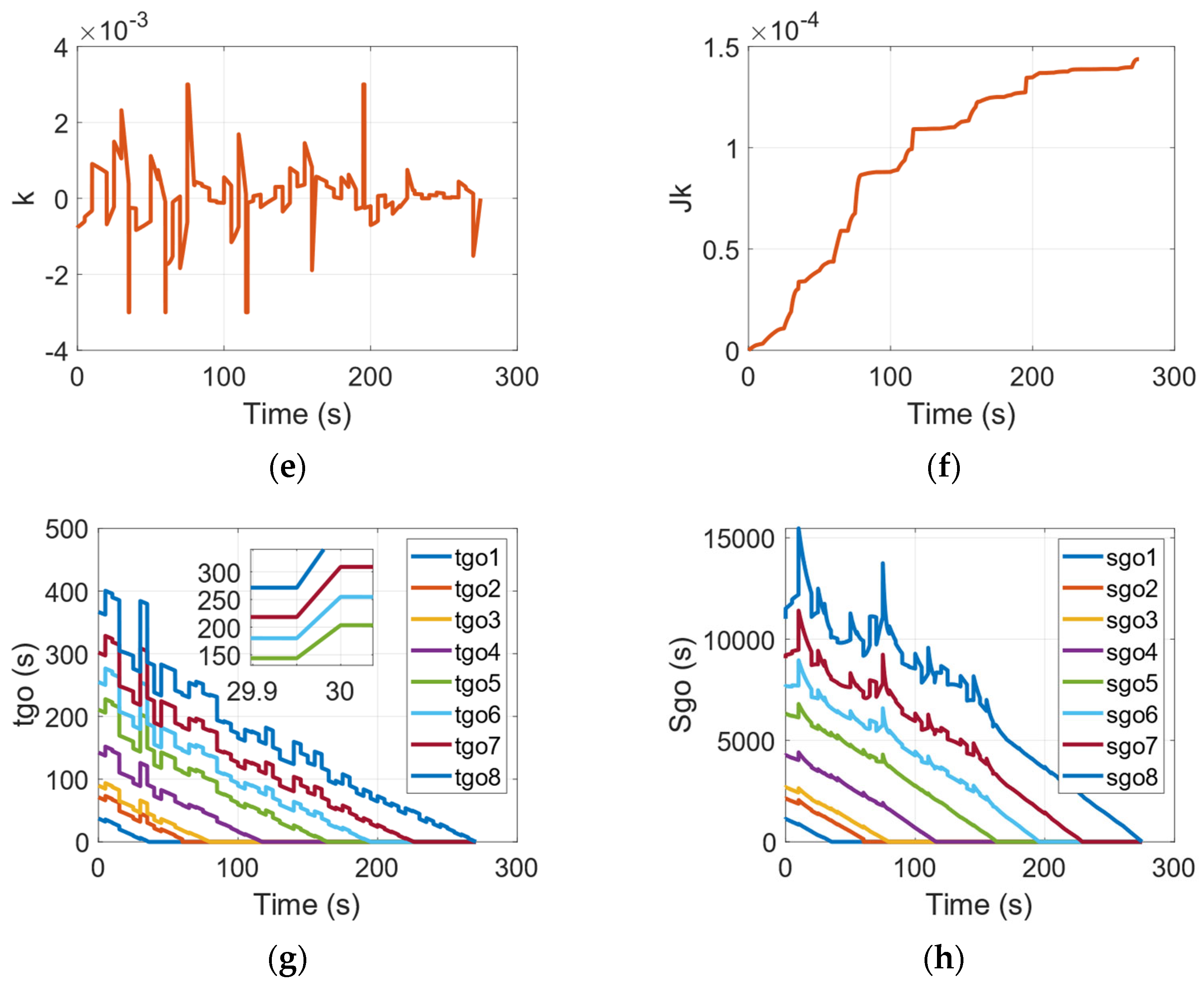
| Input: The relative range and LOS angle between the UAV and all waypoints, and , and the UAV speed . Require: . Denote: . Step 1: Compute the remaining path length . If , proceed to Step 2; otherwise, proceed to Step 3. Step 2: , . Return to Step 1. Step 3: If , proceed to Step 4; otherwise, proceed to Step 5. Step 4: Compute the remaining path length using Equation (6) (). Return to Step 1. Step 5: , Step 6: Determine the UAV’s current position. If , proceed to Step 7; otherwise, proceed to Step 8. Step 7: Compute the acceleration command k using Equation (42) and proceed to Step 9. Step 8: Step 9: Return k |
3. Numerical Simulation Results
3.1. Performance of the UAV under Varying Speeds
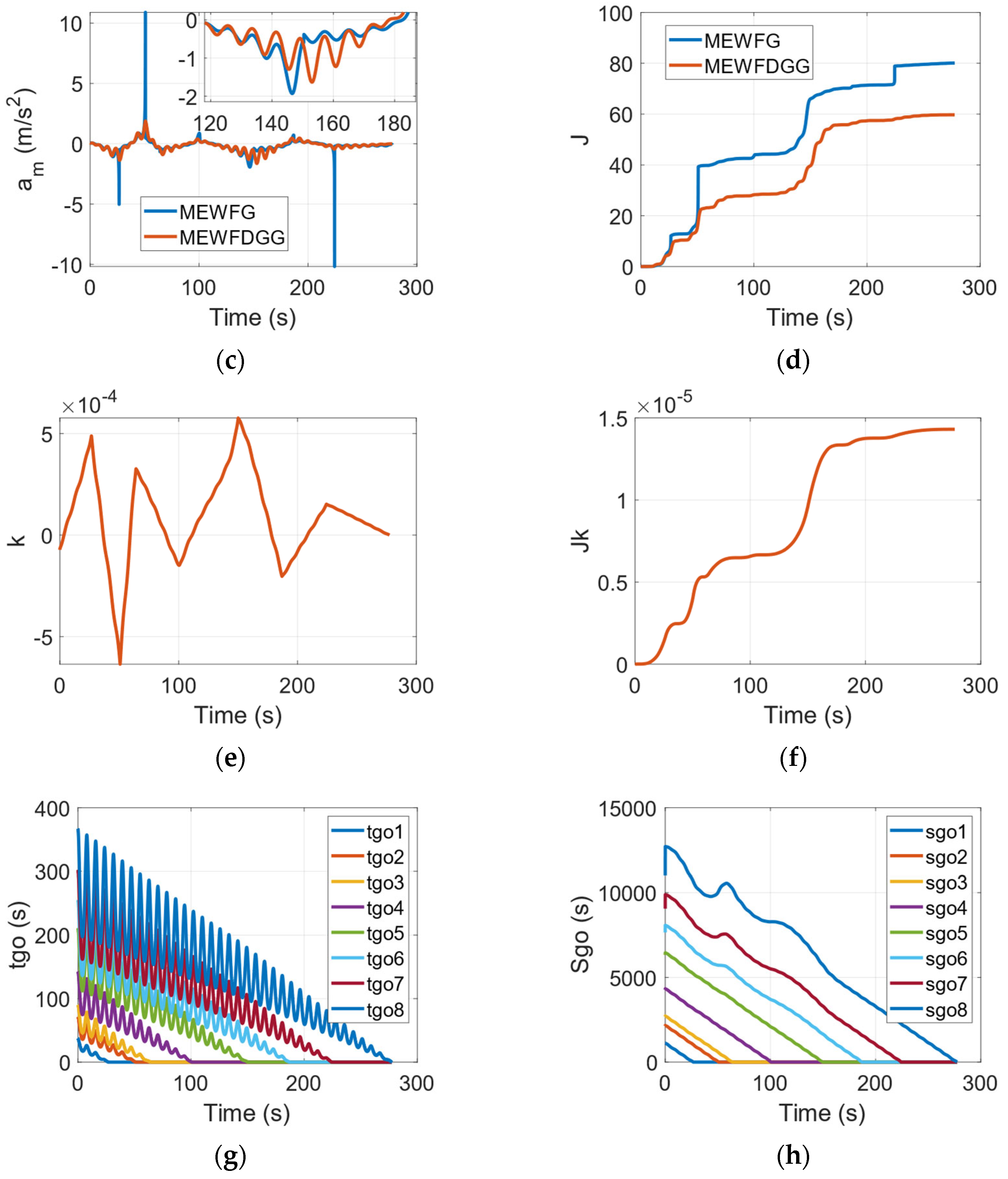
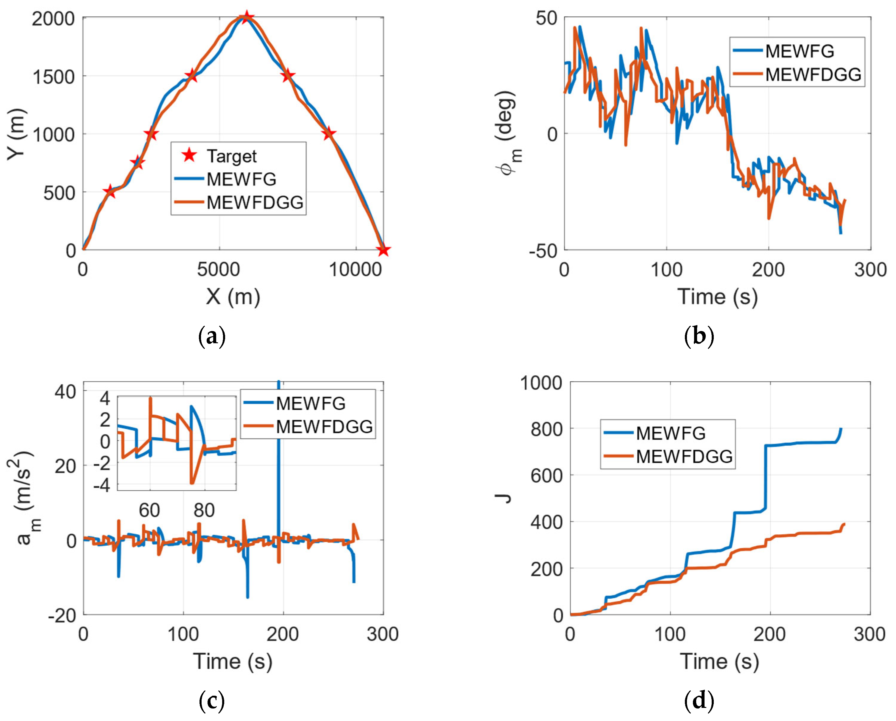
3.1.1. MEWFDGGL
3.1.2. SMEWFDGGL
3.2. Performance under the Influence of the Wind
3.2.1. MEWFDGGL
3.2.2. SMEWFDGGL
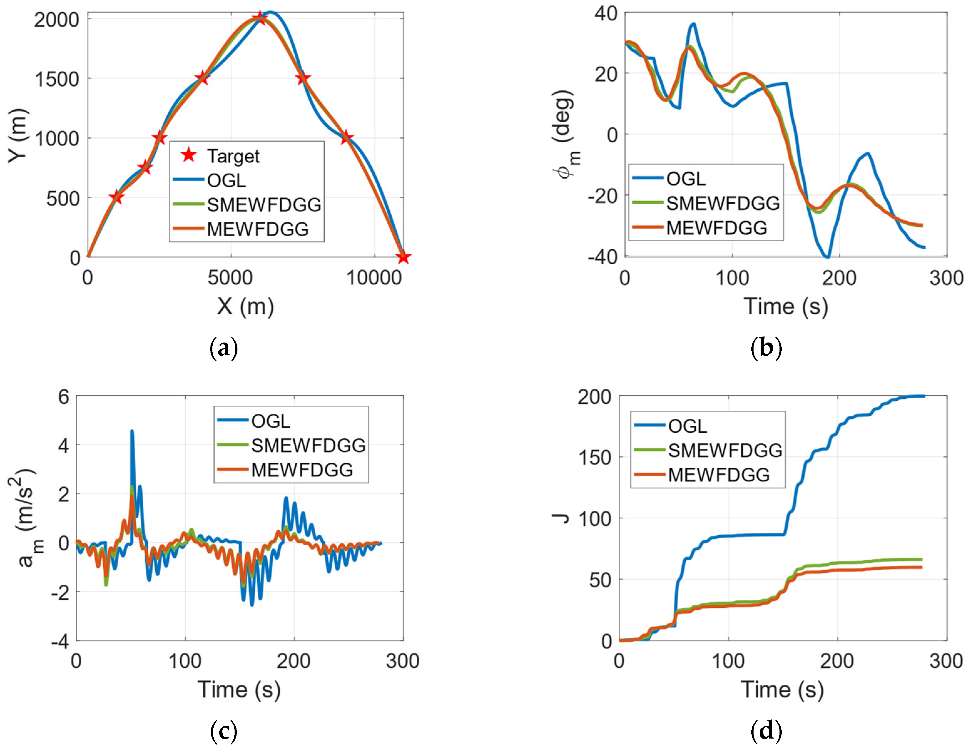
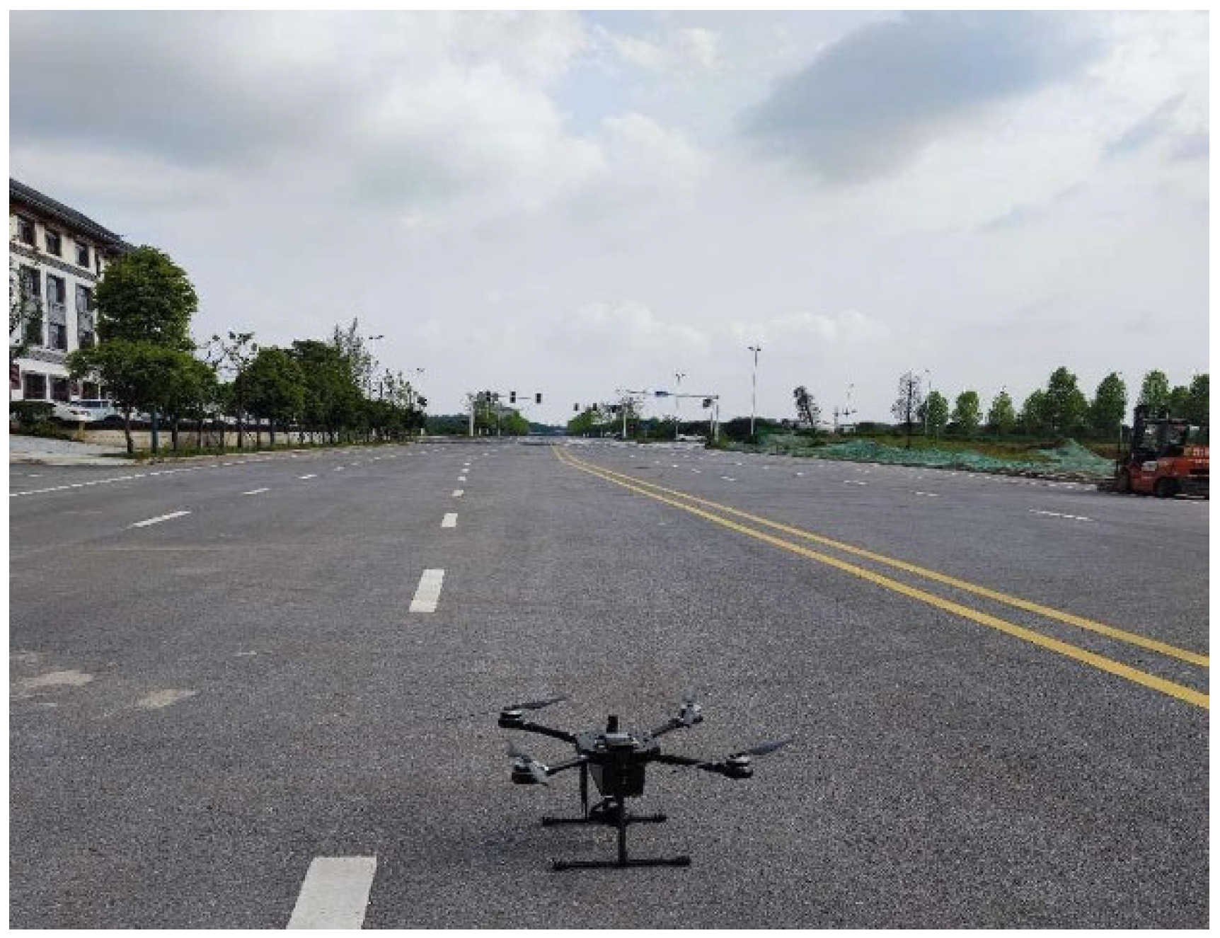
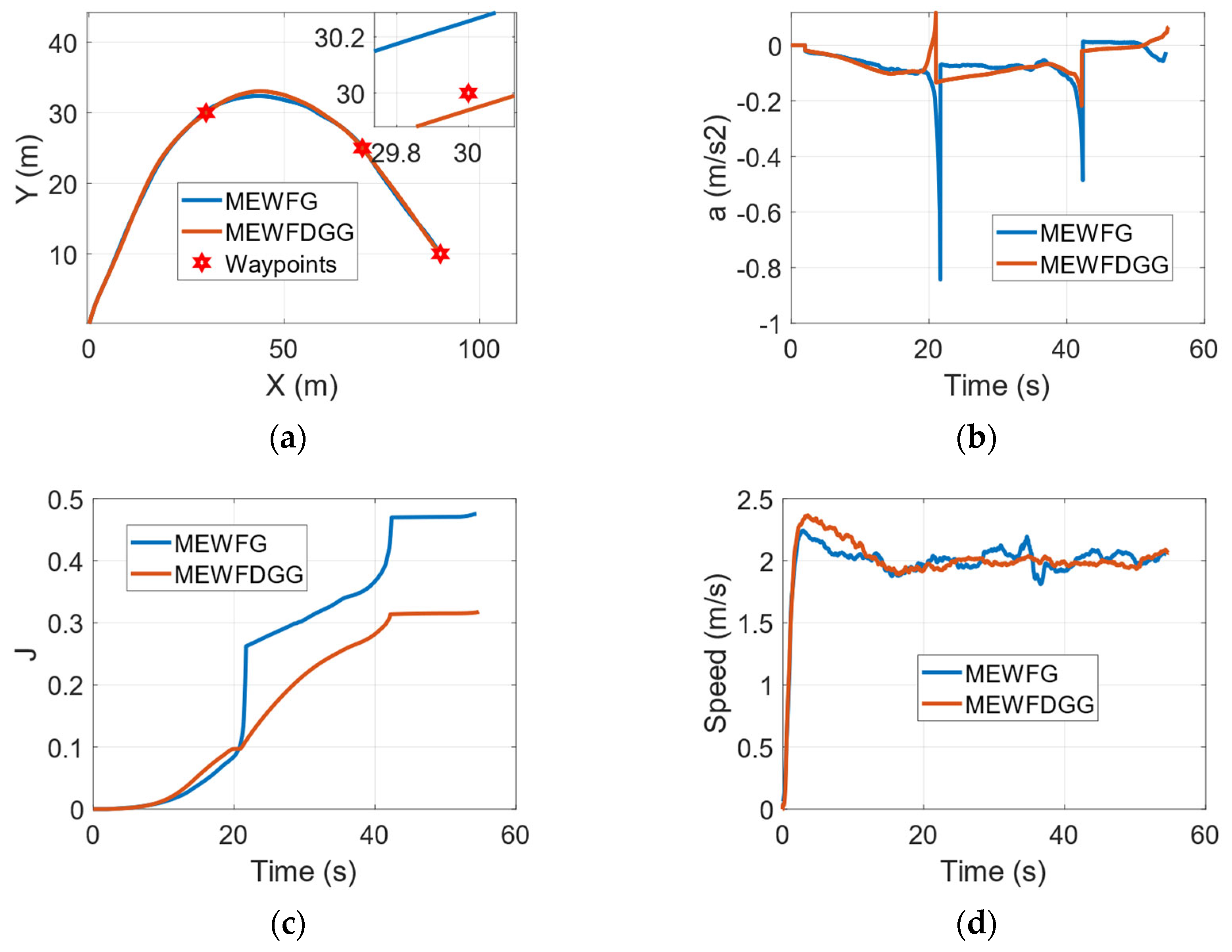
4. Experiment Verification
4.1. MEWFDGGL
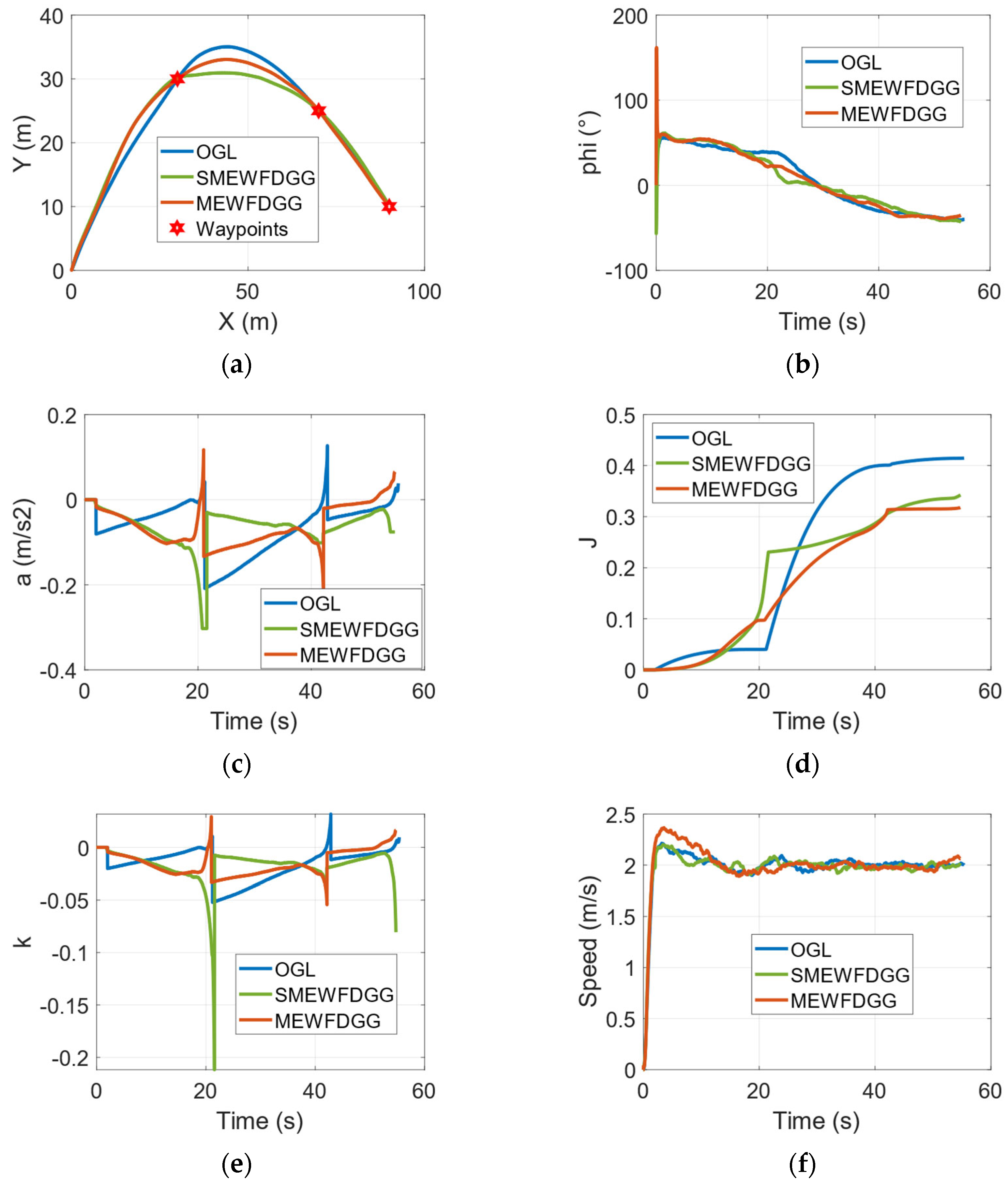
4.2. SMEWFDGGL
5. Conclusions
Author Contributions
Funding
Data Availability Statement
Conflicts of Interest
References
- He, S.; Lee, C.-H.; Shin, H.-S.; Tsourdos, A. Optimal Guidance and Its Applications in Missiles and UAVs, 1st ed.; Springer: Cham, Switzerland, 2020; pp. 151–173. [Google Scholar]
- Beard, R.W.; Ferrin, J.; Humpherys, J. Fixed Wing UAV Path Following in Wind With Input Constraints. IEEE Trans. Control. Syst. Technol. 2014, 22, 2103–2117. [Google Scholar] [CrossRef]
- Ullah, N.; Mehmood, Y.; Aslam, J.; Shaoping, W.A.N.G.; Phoungthong, K. Fractional order adaptive robust formation control of multiple quad-rotor UAVs with parametric un-certainties and wind disturbances. Chin. J. Aeronaut. 2022, 35, 204–220. [Google Scholar] [CrossRef]
- Piprek, P.; Hong, H.; Holzapfel, F. Optimal trajectory design accounting for the stabilization of linear time-varying error dynamics. Chin. J. Aeronaut. 2022, 35, 55–66. [Google Scholar] [CrossRef]
- Pang, B.; Dai, W.; Hu, X.; Dai, F.; Low, K.H. Multiple air route crossing waypoints optimization via artificial potential field method. Chin. J. Aeronaut. 2020, 34, 279–292. [Google Scholar] [CrossRef]
- Medagoda, E.D.B.; Gibbens, P.W. Synthetic-Waypoint Guidance Algorithm for Following a Desired Flight Trajectory. J. Guid. Control. Dyn. 2015, 33, 601–606. [Google Scholar] [CrossRef]
- Wang, X.; Tan, G.; Dai, Y.; Lu, F.; Zhao, J. An Optimal Guidance Strategy for Moving-Target Interception by a Multirotor Unmanned Aerial Vehicle Swarm. IEEE Access 2020, 8, 121650–121664. [Google Scholar] [CrossRef]
- Sun, G.; Wen, Q.; Xu, Z.; Xia, Q. Impact time control using biased proportional navigation for missiles with varying velocity. Chin. J. Aeronaut. 2020, 33, 956–964. [Google Scholar] [CrossRef]
- Li, K.-B.; Shin, H.-S.; Tsourdos, A.; Tahk, M.-J. Performance of 3-D PPN Against Arbitrarily Maneuvering Target for Homing Phase. IEEE Trans. Aerosp. Electron. Syst. 2020, 56, 3878–3891. [Google Scholar] [CrossRef]
- Li, K.-B.; Shin, H.-S.; Tsourdos, A.; Tahk, M.-J. Capturability of 3D PPN Against Lower-Speed Maneuvering Target for Homing Phase. IEEE Trans. Aerosp. Electron. Syst. 2019, 56, 711–722. [Google Scholar] [CrossRef]
- Kebo, L.I.; Zhihui, B.A.I.; Hyo-Sang, S.H.I.N.; Tsourdos, A.; Min-Jea, T.A.H.K. Capturability of 3D RTPN guidance law against true-arbitrarily ma-neuvering target with maneuverability limitation. Chin. J. Aeronaut. 2022, 35, 75–90. [Google Scholar]
- Zhao, Y.; Sheng, Y.; Liu, X. Trajectory reshaping based guidance with impact time and angle constraints. Chin. J. Aeronaut. 2016, 29, 984–994. [Google Scholar] [CrossRef]
- Kim, Y.-W.; Kim, B.; Lee, C.-H.; He, S. A unified formulation of optimal guidance-to-collision law for accelerating and decelerating targets. Chin. J. Aeronaut. 2022, 35, 40–54. [Google Scholar] [CrossRef]
- Qi, N.; Sun, Q.; Zhao, J. Evasion and pursuit guidance law against defended target. Chin. J. Aeronaut. 2017, 30, 1958–1973. [Google Scholar] [CrossRef]
- He, S.; Lee, C.-H.; Shin, H.-S.; Tsourdos, A. Optimal three-dimensional impact time guidance with seeker’s field-of-view constraint. Chin. J. Aeronaut. 2021, 34, 240–251. [Google Scholar] [CrossRef]
- Kyaw, P.T.; Le, A.V.; Veerajagadheswar, P.; Elara, M.R.; Thu, T.T.; Nhan, N.H.K.; Van Duc, P.; Vu, M.B. Energy-Efficient Path Planning of Reconfigurable Robots in Complex Environments. IEEE Trans. Robot. 2022, 38, 2481–2494. [Google Scholar] [CrossRef]
- Yin, Q.; Chen, Q.; Wang, Z. Energy-Optimal Waypoint-Following Guidance for Gliding-Guided Projectiles. In Proceedings of the 21st International Conference on Control, Automation and Systems (ICCAS), Jeju, Republic of Korea, 12–15 October 2021; IEEE: New York, NY, USA, 2021; Volume 34, pp. 1477–1482. [Google Scholar]
- Chen, Y.; Yu, J.; Mei, Y.; Zhang, S.; Ai, X.; Jia, Z. Trajectory optimization of multiple quad-rotor UAVs in collaborative assembling task. Chin. J. Aeronaut. 2016, 29, 184–201. [Google Scholar] [CrossRef]
- Wang, X.; Yang, Y.; Wang, D.; Zhang, Z. Mission-oriented cooperative 3D path planning for modular solar-powered aircraft with energy optimization. Chin. J. Aeronaut. 2022, 35, 98–109. [Google Scholar] [CrossRef]
- Zhou, Y.; Su, Y.; Xie, A.; Kong, L. A newly bio-inspired path planning algorithm for autonomous obstacle avoidance of UAV. Chin. J. Aeronaut. 2021, 34, 199–209. [Google Scholar] [CrossRef]
- Jeon, I.-S.; Lee, J.-I. Optimality of Proportional Navigation Based on Nonlinear Formulation. IEEE Trans. Aerosp. Electron. Syst. 2010, 46, 2051–2055. [Google Scholar] [CrossRef]
- Kim, T.-H.; Park, B.-G. Rapid Homing Guidance Using Jerk Command and Time-Delay Estimation Method. IEEE Trans. Aerosp. Electron. Syst. 2022, 58, 729–742. [Google Scholar] [CrossRef]
- Shaferman, V.; Shima, T. Linear Quadratic Guidance Laws for Imposing a Terminal Intercept Angle. J. Guid. Control. Dyn. 2008, 31, 1400–1412. [Google Scholar] [CrossRef]
- Palumbo, N.F.; Blauwkamp, R.A.; Lloyd, J.M. Modern homing missile guidance theory and techniques. Johns Hopkins APL Tech. Dig. 2010, 29, 42–59. [Google Scholar]
- He, S.; Lee, C.-H. Optimality of Error Dynamics in Missile Guidance Problems. J. Guid. Control. Dyn. 2018, 41, 1620–1629. [Google Scholar] [CrossRef]
- He, S.; Lee, C.-H.; Shin, H.-S.; Tsourdos, A. Minimum-Effort Waypoint-Following Guidance Law. J. Guid. Control. Dyn. 2019, 32, 151–173. [Google Scholar] [CrossRef]
- Kobayashi, S. Differential Geometry of Curves and Surfaces, 1st ed.; Springer: Cham, Switzerland, 2019. [Google Scholar]
- Lu, P. Intercept of Nonmoving Targets at Arbitrary Time-Varying Velocity. J. Guid. Control. Dyn. 1998, 21, 176–178. [Google Scholar] [CrossRef]
- Li, K.; Liang, Y.; Su, W.; Chen, L. Performance of 3D TPN against true-arbitrarily maneuvering target for exoat-mospheric interception. Sci. China Technol. Sci. 2018, 61, 1161–1174. [Google Scholar] [CrossRef]
- Li, K.B.; Su, W.S.; Chen, L. Performance analysis of differential geometric guidance law against high-speed target with arbitrarily maneuvering acceleration. Proc. Inst. Mech. Eng. Part G-J. Aerosp. Eng. 2019, 233, 3547–3563. [Google Scholar] [CrossRef]
- Li, K.B.; Su, W.S.; Chen, L. Performance analysis of realistic true proportional navigation against maneuvering targets using Lyapunov-like approach. Aerosp. Sci. Technol. 2017, 69, 333–341. [Google Scholar] [CrossRef]
- Shin, H.S.; Li, K.B. An Improvement in Three-Dimensional Pure Proportional Navigation Guidance. IEEE Trans. Aerosp. Electron. Syst. 2021, 57, 3004–3014. [Google Scholar] [CrossRef]


| Waypoint Number | Inertial Position (m) |
|---|---|
| 1 | (1000, 500) |
| 2 | (2000, 750) |
| 3 | (2500, 1000) |
| 4 | (4000, 1500) |
| 5 | (6000, 2000) |
| 6 | (7500, 1500) |
| 7 | (9000, 1000) |
| 8 | (11,000, 0) |
| Guidance | MEWFG | MEWFDGGL |
|---|---|---|
| Maximum ZEM (m) | 0.02 | 0.0018 |
| Maximum acceleration command (m/s2) | 10.17 | 1.891 |
| Energy consumption | 80.09 | 59.71 |
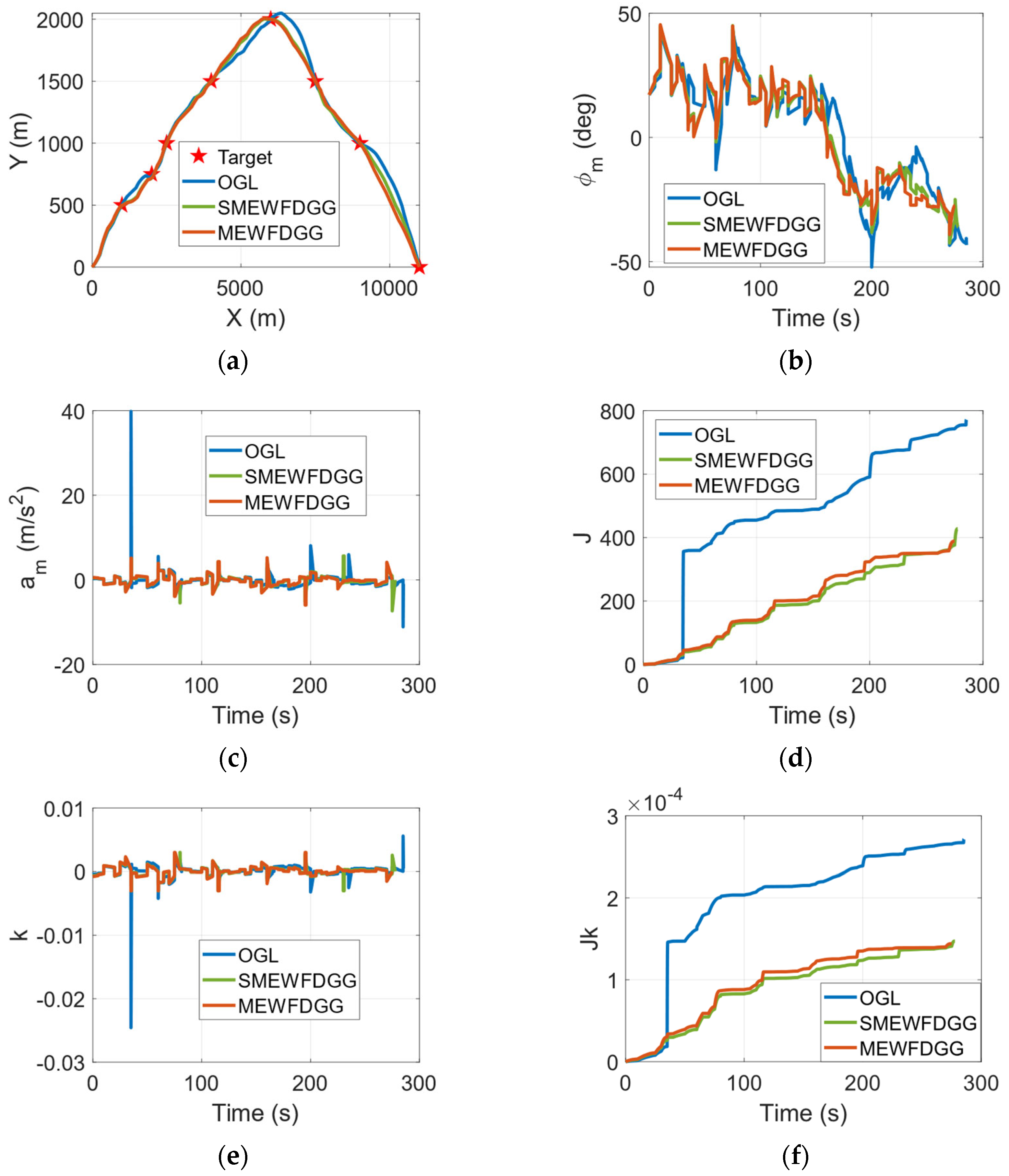
| Guidance | OGL | MEWFDGGL | SMEWFDGGL |
|---|---|---|---|
| Maximum ZEM (m) | 0.00001 | 0.0018 | 0.0015 |
| Maximum acceleration command (m/s2) | 4.552 | 1.891 | 2.271 |
| Energy consumption | 199.5 | 59.71 | 66.21 |
| Guidance | MEWFG | MEWFDGGL |
|---|---|---|
| Maximum ZEM (m) | 0.1507 | 0.0488 |
| Maximum acceleration command (m/s2) | 42.4 | 5.247 |
| Energy consumption | 802.2 | 388.1 |
| Guidance | OGL | MEWFDGGL | SMEWFDGGL |
|---|---|---|---|
| Maximum ZEM (m) | 0.001 | 0.04883 | 0.0532 |
| Maximum acceleration command (m/s2) | 9.79 | 5.247 | 7.336 |
| Energy consumption | 754.8 | 388.1 | 427.7 |
| Waypoint Number | Inertial Position (m) |
|---|---|
| 1 | (30, 30) |
| 2 | (70, 25) |
| 3 | (90, 10) |
| Guidance | MEWFG | MEWFDGGL |
|---|---|---|
| Maximum ZEM (m) | 0.25 | 0.06 |
| Maximum acceleration command (m/s2) | 0.843 | 0.1173 |
| Energy consumption | 0.4753 | 0.3176 |
| Guidance | OGL | MEWFDGGL | SMEWFDGGL |
|---|---|---|---|
| Maximum ZEM (m) | 0.02 | 0.06 | 0.17 |
| Maximum acceleration command (m/s2) | 0.2086 | 0.2177 | 0.3029 |
| Energy consumption | 0.4146 | 0.3174 | 0.3423 |
Disclaimer/Publisher’s Note: The statements, opinions and data contained in all publications are solely those of the individual author(s) and contributor(s) and not of MDPI and/or the editor(s). MDPI and/or the editor(s) disclaim responsibility for any injury to people or property resulting from any ideas, methods, instructions or products referred to in the content. |
© 2023 by the authors. Licensee MDPI, Basel, Switzerland. This article is an open access article distributed under the terms and conditions of the Creative Commons Attribution (CC BY) license (https://creativecommons.org/licenses/by/4.0/).
Share and Cite
Qin, X.; Li, K.; Liang, Y.; Liu, Y. Minimum-Effort Waypoint-Following Differential Geometric Guidance Law Design for Endo-Atmospheric Flight Vehicles. Drones 2023, 7, 369. https://doi.org/10.3390/drones7060369
Qin X, Li K, Liang Y, Liu Y. Minimum-Effort Waypoint-Following Differential Geometric Guidance Law Design for Endo-Atmospheric Flight Vehicles. Drones. 2023; 7(6):369. https://doi.org/10.3390/drones7060369
Chicago/Turabian StyleQin, Xuesheng, Kebo Li, Yangang Liang, and Yuanhe Liu. 2023. "Minimum-Effort Waypoint-Following Differential Geometric Guidance Law Design for Endo-Atmospheric Flight Vehicles" Drones 7, no. 6: 369. https://doi.org/10.3390/drones7060369