1. Introduction
In the era of 5G and the upcoming 6G, the demand for UAVs in public safety and other fields is increasing. UAVs equipped with infrared thermal dual-light cameras play an important role in smart city aerial intelligence, providing a practical solution for large-scale urban patrols. Smart city aerial intelligence is a feasible and cost-effective solution to address the challenges of large inspection and supervision areas, heavy inspection tasks, and limited frontline inspection staff in the process of urban governance, reducing potential safety hazards and illegal incidents [
1]. Multi-UAV coordinated trajectory planning for large urban patrols is crucial in the process of autonomous patrol tasks performed by multiple UAVs and directly impacts the efficiency of patrol missions. It is the key to autonomous patrol tasks performed by UAVs [
2].
The use of UAVs encompasses a wide range of applications, such as monitoring tasks [
3], logistics distribution [
4], warehousing [
5], and industrial [
6] operations, among others. At this stage, although there has been much research on UAV patrols [
7], efficient UAV patrol path-planning algorithms in cities are almost missing. Yao et al. [
8] developed a new algorithm based on disturbing fluid and trajectory propagation to solve the problem of UAV’s three-dimensional path planning in a static environment. Xia et al. [
9] established a trajectory optimization model based on uniform time intervals and proposed a gradient-based sequential minimum optimization (GB-SMO) algorithm to solve the UAV planning problem. Gao et al. [
10] also studied trajectory planning for battlefield missions based on the war environment, based on the improved RRT algorithm, with the shortest trajectory and the shortest planning time as the goal. The above studies have carried out useful explorations on multi-UAV trajectory planning based on various backgrounds; however, none of them involve the field of urban patrol. Further, Wang et al. [
11] proposed a heuristic algorithm for urban road network surveillance tasks to study multi-aircraft trajectory planning for rotary-wing UAVs. In addition, Zhang et al. [
12], based on the urban mission background, aimed at the problem that UAV flying in the urban environment posed a greater threat to pedestrians and public property and established a mathematical model of UAV trajectory planning with the introduction of risk assessment. Further, they proposed an improved ant colony algorithm for optimal trajectory planning and achieved certain results. Na et al. [
13], on the other hand, focused on 3D path optimization and real-time obstacle avoidance of UAVs based on the urban context. Muñoz et al. [
14] instead focused on the formation control of UAVs in cities. Wang et al. [
15] also studied UAV flight planning based on the urban environment and hybrid strategy to ensure the smooth progress of urban flight. In addition, there is still much research on UAV trajectory planning based on the urban environment [
16,
17]. The above studies have all made significant contributions to the field of urban patrol. However, their research objectives are limited to the shortest trajectory and the maximum safety factor, task completion rate, and other issues.
Involving the UAV trajectory planning algorithm, Dai et al. [
18] used the genetic algorithm to plan the path of the UAV in small-scale trajectory planning problems. Yuan et al. [
19] added pheromone and heuristic functions to the traditional particle swarm algorithm to realize the path planning of UAVs. He et al. [
20] proposed a novel hybrid algorithm called HIPSO-MSOS by combining Improved Particle Swarm Optimization (IPSO) and Modified Symbiotic Search (MSOS). There are also methods based on the mixed integer linear programming (MILP) method [
21], the hybrid genetic and A* algorithm [
22], the improved CSA algorithm [
23], the PIOFOA algorithm [
24], etc. However, these methods are not applicable for multi-UAV trajectory planning under multiple constraints, as it is difficult to find an optimal solution. The biological heuristic algorithm is widely used in large-scale optimization problems, such as multi-aircraft cooperative trajectory planning, due to its excellent characteristics [
25,
26,
27]. Sun et al. [
28] used the bat algorithm to optimize UAV mission planning. Duan et al. [
29] proposed a dynamic discrete pigeon-inspired optimization algorithm based on multi-UAV coordinated trajectory planning in a three-dimensional environment. Jain et al. [
30] used the multi-universe algorithm to research UAV trajectory planning in a dynamic environment. The above research on various UAV trajectory planning algorithms has carried out a useful exploration to optimize UAV trajectory with certain reference significance. The lightning search algorithm [
31], a new biological heuristic algorithm, has the advantages of a simple structure and a short calculation time. However, when applied to the three-dimensional trajectory planning of UAVs, the search accuracy is low, and it is easy to fall into optimal local values, resulting in the problem of algorithm premature convergence. Therefore, this paper aims to improve the shortcomings of the lightning search algorithm, which are that it is easy to fall into the local optimum and the uniformity is not good enough.
Based on the studies mentioned above, this paper aims to establish a multi-rotor UAV-coordinated mission planning model for urban patrol. The model incorporates a multi-objective function that considers the least impact cost of UAVs, the shortest UAV flight energy consumption cost, and the highest UAV mission execution rate. This paper introduces a multi-level nesting strategy and random walk strategy to improve the global search ability and convergence accuracy of the lightning search algorithm (LSA). Furthermore, the improved algorithm is combined with the RRT algorithm, which introduces the greedy strategy to overcome the problems of falling into the optimal local solution and slow convergence speed when solving the trajectory planning problem. Finally, a real patrol environment based on a satellite image of a specific location in Beijing is established to verify the effectiveness of the proposed multi-rotor UAV urban patrol mission trajectory planning program. The simulation results show that the proposed algorithm has fast convergence speed and high accuracy compared with LSA and other algorithms. It can efficiently plan the trajectory for UAVs performing urban patrol tasks, thereby improving the urban patrol efficiency of the multi-rotor UAV. The UAV to perform patrol tasks schematic is shown in
Figure 1.
The remainder of this paper is organized as follows. The urban environment model, UAV cost model, etc., are built in
Section 2, modeling of UAV mission planning, which introduces the concept and necessity of urban patrol. Urban environment modeling establishes the environment model of the city. Trajectory cost modeling establishes the UAV cost model for urban patrol. Quadrotor UAV system modeling is built in
Section 3, quadrotor UAV system modeling. The improvement strategy of the RRT algorithm and the process and improvement based on the lightning search algorithm is described in
Section 4, algorithm description based on multi-layer nesting and randomized swimming strategy. The simulated data and graphs are shown in
Section 5, simulation results. Simulation results conduct experimental simulations by the improved RRT algorithm. The conclusion draws conclusions. Finally, the conclusions and contributions of this paper based on the simulation results are in
Section 6, conclusions and future research.
Figure 1.
The UAV to perform patrol tasks schematic.
Figure 1.
The UAV to perform patrol tasks schematic.
2. Modeling of UAV Mission Planning
In this section, the mission description of UAV city patrol is first introduced, then the environmental model is established, and a multi-UAV mission planning model that considers UAV mission execution rate, flight energy consumption cost, and impact cost are developed.
2.1. Problem Description
As smart cities move towards high-quality construction and development, the demand for intelligent information control is increasing. UAVs can conduct comprehensive surveys and maps of urban management effects at different times, providing the government with accurate and objective bases for urban management. The specific tasks of UAV patrol operations in large cities are as follows: Each UAV departs from the same center and returns to the center after completing all missions, flying according to the established planned route and not accepting new mission assignments. The urban environment is complex, with many pedestrians and vehicles, and a crash can cause damage to pedestrians and vehicles. Therefore, it is necessary to ensure that all patrol tasks are carried out under the premise of the minimum danger to the public in the event of a crash and with the shortest trajectory as the goal. Ultimately, a flight path with full coverage of the patrol area is planned for multiple UAVs.
2.2. Urban Environment Modeling
In a complex and dense urban environment, UAV patrols encounter a wide variety of obstacles, unevenly distributed and restricted by the complex constraints of the airspace environment. Three-dimensional environment modeling solves the prerequisite of UAV path planning. To improve the efficiency of UAV planning, create a simplified modeling diagram of the city’s three-dimensional space. Simplify various obstacles into rectangular bodies, and perform environmental modeling after simplifying all buildings, just like
Figure 2. All buildings are avoidance areas for UAVs to fly, and the plane coordinates of the
building are expressed as
. The height is expressed as
,
and it is the number of plane coordinates of
building coordinates. Where
,
is the number of buildings. Avoidance area constraints of ground UAVs are
2.3. Trajectory Cost Modeling
Building upon the mathematical model proposed by Zhang et al. [
8], this paper introduces a cost-effectiveness ratio of UAVs equipped with infrared thermal dual-light cameras to enhance urban patrols’ efficiency and minimize energy consumption. It should be noted that the assumptions in this study are limited to urban architectural environments and do not account for geographical features, such as mountains and basins. The UAV impact cost formula is presented below:
The UAV impact cost formula includes several variables. represents the impact cost of the UAV in case of a fall. denotes the reliability factor of the UAV. reflects the density of vehicles per unit area while represents the density of population per unit area. indicates the death rate of the population due to car accidents. and are the highest-flying height and true flying height of the UAV, respectively.
The formula for UAV flight energy consumption cost with
representing the energy consumed per unit distance of flight is presented below:
2.4. UAV Mission Execution Rate
The infrared thermal dual-lens camera is equipped with a 25 mm lens, 90° infrared light, and a shooting angle of 90°, with the best observation distance being between 50–100 m. The objective is to maximize the patrol area of each UAV while minimizing the repetition rate of patrols. The patrol area of each UAV is presented below:
where
is the track length of each UAV.
is the flying height of each UAV.
is the maximum coverage angle that the UAV equipped with the camera can shoot on the vertical plane. Where
represents the track length of each UAV,
denotes the flying height of each UAV, and
indicates the maximum coverage angle that the camera-equipped UAV can capture on the vertical plane.
where
represents the patrol repetition rate of the two UAVs,
is the flight distance between the two UAVs, and
is defined as the minimum distance between any two UAVs to avoid repeated patrols.
Therefore, the objective function is as follows:
This is expressed as the lowest impact cost and UAV flight energy consumption cost, the largest patrol area, and the lowest UAV patrol repetition rate in the route from departure to return when multiple UAVs are dispatched for urban patrol missions.
2.5. Restrictions
Based on the three-dimensional city map established in
Section 2 and the trajectory objective function established in the previous section, the following constraints are formulated.
UAV flight range constraints. UAV patrols are restricted by relevant legal supervision and other factors, and there are space restrictions on patrol areas. Let
,
,
,
,
, and
be the minimum and maximum spatial locations that the relevant laws allow UAVs to reach. The constraint is expressed as the following:
where
,
,
,
,
, and
are the space limits for UAVs to perform patrol missions.
Limitations of UAV flying height. There exists a minimum flight height
and a maximum flight height
for UAV manufacturing specifications to ensure flight safety when performing patrol tasks, which are constrained to be expressed as the following:
UAV range restrictions. The energy carried by UAVs is limited, and there is a maximum range limit. Let
be the maximum energy the UAV possesses before taking off. The constraint is expressed as the following:
Patrol area coverage limit. When the UAV performs a patrol mission, subject to the mission requirements, the UAV patrol coverage area needs to be larger than the other mission requirements.
According to the patrol mission requirements, the minimum patrol area is defined as
. The corresponding constraint can be expressed as the following:
UAV navigation angle constraints are shown below:
In Equation (13), is the turning angle at position . When the UAV performs a turning operation, it satisfies . Equation (14) is the turning angle constraint of the UAV, where is the maximum turning angle of the UAV. In Equation (15), is the climb angle at position . When the UAV is performing a climb operation, . Equation (16) is the climb angle constraint of the UAV, where is the maximum climb angle of the UAV.
4. Algorithm Description
This section proposes two improvements to the RRT algorithm for UAV trajectory planning. Firstly, the greedy strategy is integrated into the RRT algorithm. Secondly, the lightning search algorithm is enhanced by introducing multi-layer nesting and random walk strategy, which is combined with the improved RRT algorithm for UAV mission planning.
4.1. RRT Algorithm Optimized by Greedy Strategy (GP-RRT)
The RRT algorithm is currently considered the most advanced method for UAV path planning. It is particularly effective in navigating unexplored areas with ample space and few obstacles. However, due to its exhaustive search approach, it may not be suitable for directing UAVs to specific points. Therefore, to improve exploration efficiency and avoid blind search, we propose a greedy strategy that modifies the exploration path. This approach reduces exploration time, shortens the search path, and eliminates the search for unproductive blank areas.
4.1.1. Impact Checking
To prevent UAVs from colliding with 3D terrain, set the collision detection rules according to the terrain as follows:
where the output is
for no collision and
for a collision with the building.
represents a new location node and
represents a set of location points where the building is located.
4.1.2. Greedy Policy Detection
Simulation experiments are required to solve and validate the established model. The model includes limits on the mission execution rate and calculates the patrol repetition rate between UAVs. An optimization algorithm is used to obtain the optimal path of the UAV. In the context of RRT, if the initial path is generated using the traditional algorithm, the direction of optimization can be too large, making it difficult to quickly and efficiently find a better path. To address this issue, we propose using the sampling points of the target paranoid function for optimization while also adjusting the probability of the new node location to avoid invalid searches. In addition to the greedy strategy, we also incorporate a local expansion mechanism. This mechanism involves removing new nodes within the already traversed area in the existing node region. By doing so, we further enhance the optimization of the greedy strategy. The formula for updating nodes is as follows:
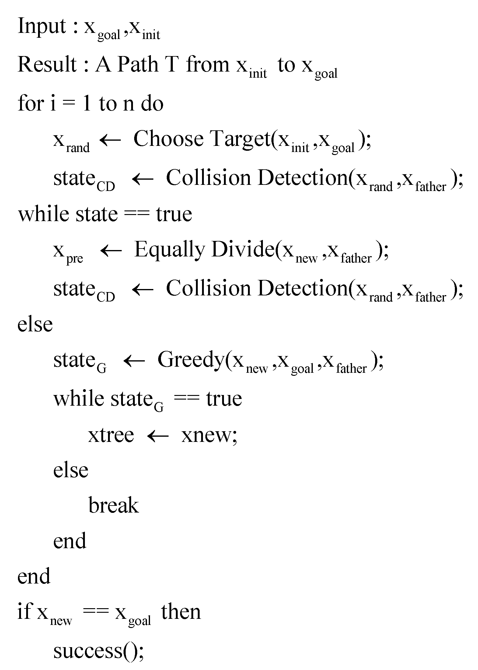
The improvement strategy steps are as follows.
Step 1: randomly expand the tree to generate a new node .
Step 2: perform collision detection.
Step 3: If there are no obstacles, perform greedy policy detection. If the greedy rule is met, add to . If the greedy rule is not met, return to Step 1.
Step 4: If there is an obstacle, connect to the parent node . Divide the line segment into 2 equal parts, mark it as , and return to Step 2.
Step 5: Repeat Steps 1–4 until reaching the target point.
The output includes the detection results for collision detection
, the result of collision detection
, and the result of greedy detection
, as well as the number of iterations
. The pseudocode of the algorithm is shown in
Figure 4.
The schematic diagram of the process is shown in
Figure 5.
4.2. Lightning Search Algorithm Based on Multi-Level Nesting and Random Walk Strategy (MNRW-LSA)
In the field of multi-UAV path planning, there exist numerous optimization algorithms to solve such problems. However, the key challenges in the UAV trajectory cost model are the coverage rate and repetition rate, which are more difficult to address. Multi-UAV collaborative patrol tasks are complex and involve issues such as information interaction and path prioritization. It is essential for the individuals involved to possess diverse properties to enhance the effectiveness of the optimization algorithm. We suggest utilizing an enhanced version of the lightning search algorithm (LSA) to resolve the model. LSA mimics the natural occurrence of lightning discharge in the environment. According to the lightning conduction mechanism, there are three types of discharges: transient, spatial, and guided. Each type has unique discharge characteristics, and their probabilistic and detour characteristics can be utilized to optimize individual space.
This paper introduces a solution to the problem of weak random performance and low traversal coverage in the spatial search of an individual gradient optimization mechanism. The proposed solution involves implementing random touring based on the original algorithm and performing multi-layer nesting operations to achieve end re-optimization. A lightning search algorithm based on multi-layer nesting and random touring strategy is proposed as a way to complete the solution of the model.
4.2.1. Algorithm Principle
Transient Discharger
A transient discharger is a random-direction discharge body. Therefore, it can be considered a random number obtained from the standard uniform probability distribution on the open interval of the solution space—these dischargers whose positions satisfy the problem to be optimized. Generate an initial population that obeys a uniform distribution, and the population size is
. The probability density function of standard uniform distribution:
where
is a random number that can provide a candidate solution.
and
are the lower and upper bounds of the solution space.
Spatial Discharger
Transition dischargers form the next channel. Let the position of the spatial discharger be
. Randomly generated numbers using an exponential distribution function with an exponential distribution probability density function:
represents the position of the space discharge body and represents the solution in the calculation formula. The position of the spatial discharger or the direction of the next iteration can be controlled by the shape parameter
.
at the
iteration position can be described as the following:
where
is exponential random numbers, and if
is negative, then the resulting random number should be subtracted because Equation (40) only provides positive values.
However, the new position does not guarantee channel formation unless is a better solution. If provides a better solution in the next step, then will be updated to , otherwise it will remain unchanged. If is better than the current iteration, then the spatial discharger becomes guide discharger.
Guide Discharger
Randomly generated numbers using a normal distribution with a normal distributions probability density function:
The randomly generated guide discharger can be searched in all directions from the current position defined by the shape parameter, and its mining capacity can be defined by the scale parameter.
and
represent the shape parameter and scale parameter in the normal distribution, respectively. The shape parameter
of the induced discharge
exponentially decreases as it advances toward the Earth or finds the optimal solution. The position of the guide discharge
at the
iteration can be described as the following:
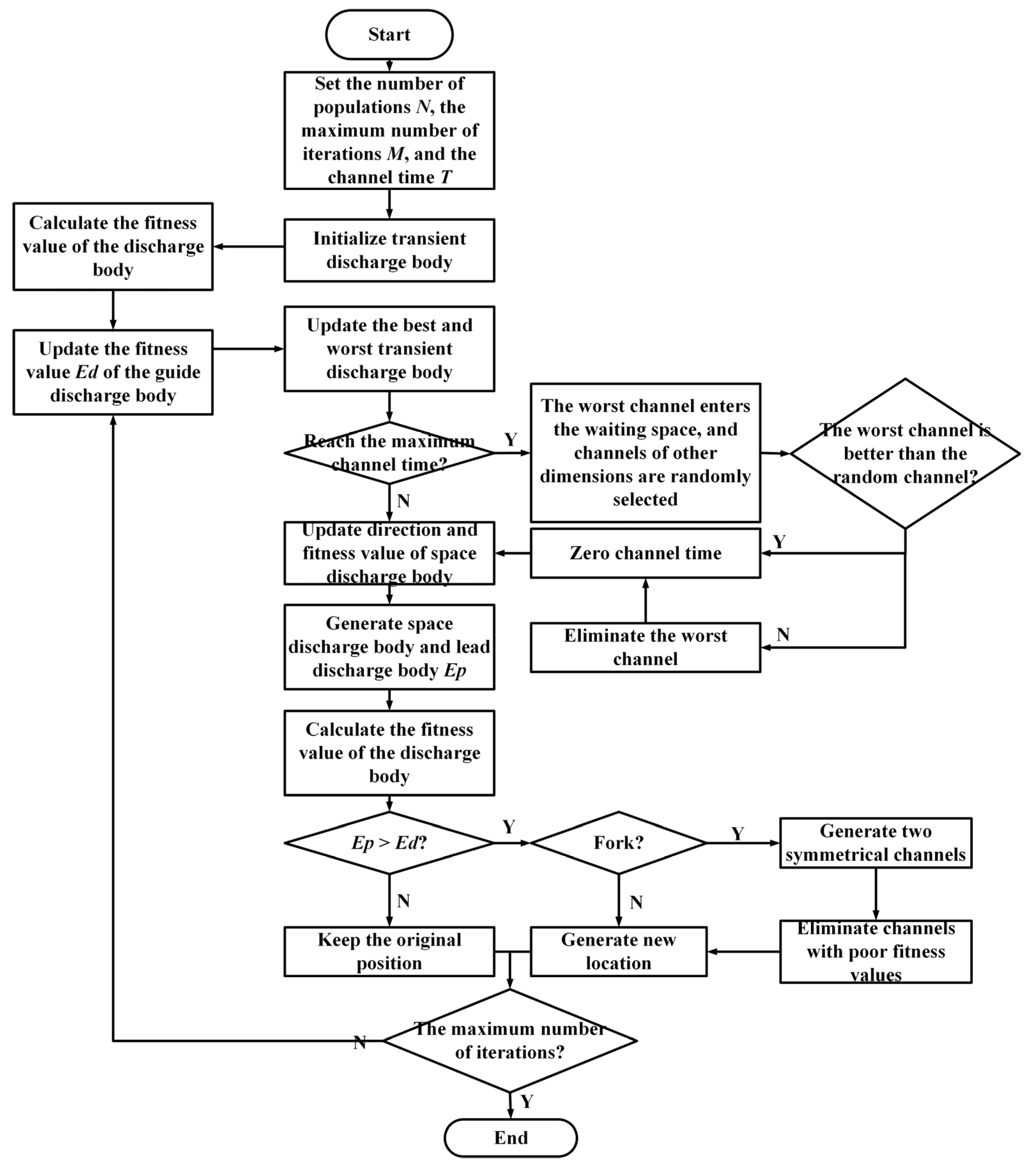
The basic lightning search algorithm steps are as follows.
Step 1: initialize the parameters, and set the number of races , the maximum number of iterations , and channel time .
Step 2: initialize the transition discharger and calculate the fitness value of the discharger.
Step 3: update the fitness value of the guide discharger.
Step 4: update the best and worst transition dischargers and record the channel time.
Step 5: if the maximum channel time is reached, the worst channel is eliminated, and the channel time is reset to zero.
Step 6: update the conduction time and the fitness value of the discharger, and generate the spatial discharger and the guide discharger.
Step 7: update the transition discharger.
Step 8: If the maximum number of iterations is reached, the best discharge body is output; if the maximum number of iterations is not reached, return to Step 2.
4.2.2. Multi-Level Nested Synchronization Optimization Mechanism
In this study, we propose a multi-layer nested synchronization optimization mechanism to address the challenge of optimizing the paths of multiple UAVs during collaborative patrols. While it is relatively easy for UAVs to exchange information with each other, optimizing the coverage, cost, and repetition rate of each UAV patrol is a complex task. Our approach considers these factors and aims to find an optimal solution. The algorithm has been optimized by storing the optimized and unoptimized parts in separate spaces. This approach is superior to traditional optimization methods and makes the algorithm more effective in solving the model.
In the above at Step 5, if the renewal of the transient discharge body is not completed within the maximum conduction time, the time channel is eliminated. However, at the maximum conduction time, the transient discharge body of this time channel is superior to that of any other time channel. This paper utilizes a multi-level nesting operation in Step 5 to enhance the performance of the algorithm to prevent the loss of a more efficient discharge channel.
The implementation steps are as follows.
Step 1: put the location, X, of the discharge body in the time channel eliminated in Step 5 into the additional generated storage space.
Step 2: Randomly select the position of the discharge body in other time channels. If its position is better than x, the time channel will be eliminated.
Step 3: If x is better than the randomly selected discharge body position, the time is reset to zero, but the time channel is not eliminated.
The algorithm’s pseudo code is shown in
Figure 6.
4.2.3. Random Walk Strategy
After obtaining the initial path using the improved RRT algorithm, direct path optimization often leads to duplicated patrol paths and a high repetition rate. However, utilizing the random touring strategy can effectively expand the search space and increase path diversity while still optimizing the path.
The discharge body obtained in Steps 5–7 does not have a definite time channel. In Step 8, if the maximum number of iterations is not reached, the conduction time will be increased, and the next cycle will be entered. This will disperse the positions of the better individuals. This paper proposes using a random walk strategy to concentrate the better discharge bodies and optimize their channels to address this. The set with the largest number of optimal discharge bodies is the most optimized area.
The position of the random walk strategy is updated as follows:
where
is the
-th solution of the
-th generation.
and
are two random solutions of the
-th generation.
is the scaling factor, and its range is
.
The flow chart of the MNRW-LSA algorithm is shown in
Figure 7.
5. Simulation Results
In this section, the proposed MNRW-LSA algorithm is tested with eight benchmark functions and Friedman and Nemenyi tests. Moreover, a validity test of the GP-RRT algorithm was also conducted. Finally, the proposed model is simulated by the improved algorithm and compared with multiple algorithms, then further analyzed and verified according to the experimental results.
5.1. Algorithm Improvement Strategy Verification and Multi-Algorithm Data Comparison Analysis
First, to evaluate the improvement of the LSA by the strategy proposed in this paper, we first selected several typical test functions for comparison experiments, comparing GJO, HPO, POA, RSA, and LSA with the MNRW-LSA proposed in this paper, where the dimensionality is Dim = 30. The objective functions for conducting the tests and testing standards are shown in
Table 1 and
Table 2 [
32,
33,
34,
35].
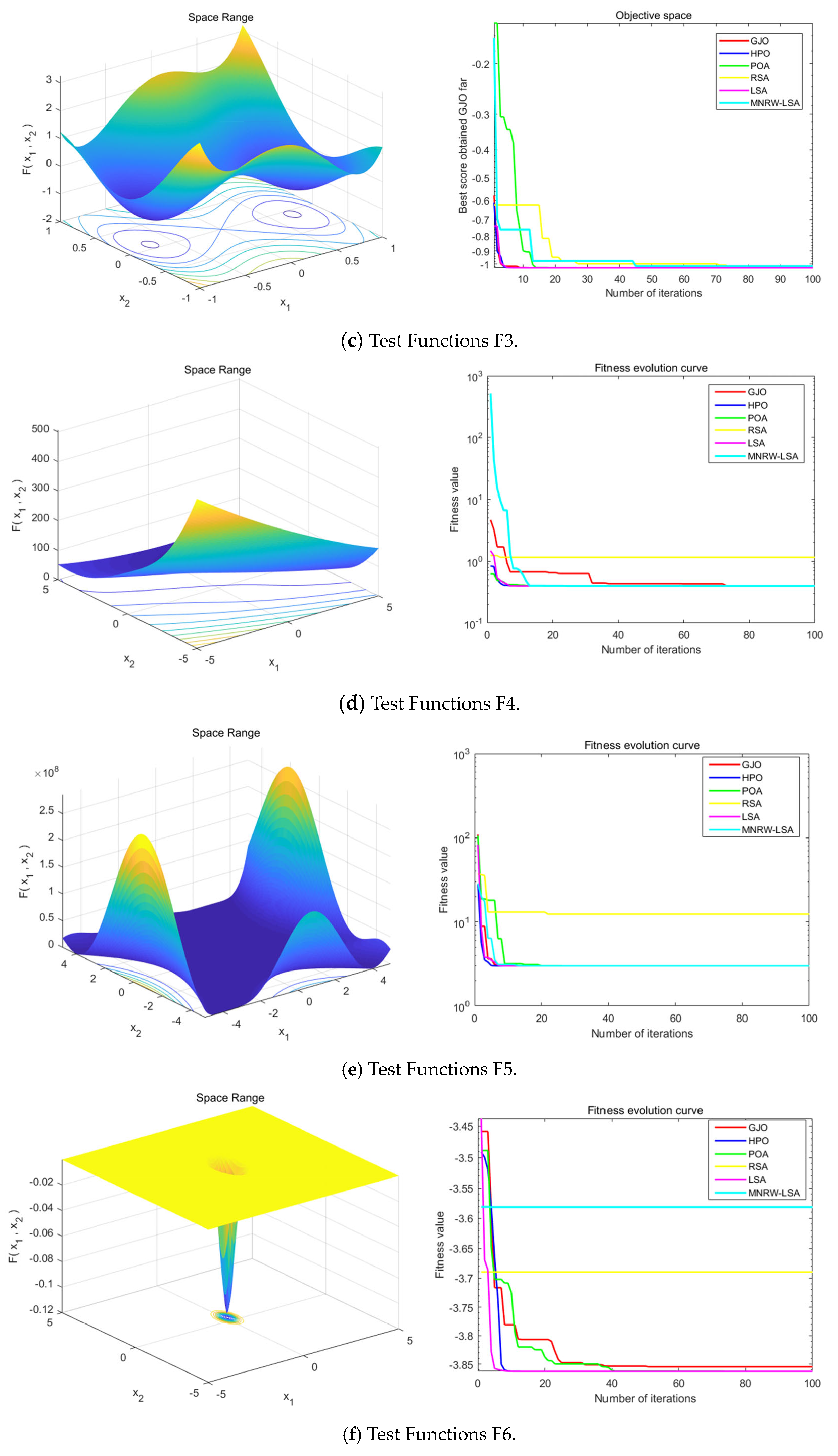
Figure 8 represents the search space range of the eight composite benchmark test functions, the fitness evolution curve of the MNRW-LSA algorithm, and the other four latest algorithms published in 2022. The 3D search space range visually reflects the solution value region within the range of values, and the curve plots clearly compare the performance of the algorithms. It can be seen from
Table 3 that the MNRW-LSA algorithm proposed in this paper achieves the optimal solution value six out of eight times with the test results of different composite benchmark test functions. The results show the optimization performance of the MNRW-LSA algorithm in the composite function and prove that the MNRW-LSA algorithm can be used in other optimization problems.
Table 3.
Comparison table of test results.
Table 3.
Comparison table of test results.
| Functions | Theoretical Minimum Value | Optimization Result Value | Is the MNRW-LSA Algorithm Optimal? |
|---|
| GJO | HPO | POA | RSA | LSA | MNRW-LSA |
|---|
| F1 | 1 | 0.998 | 0.998 | 0.998 | 11.14 | 0.998 | 12.67 | 0 |
| F2 | 0.1484 | 0.0003483 | 0.0003133 | 0.0003075 | 0.09601 | 0.001293 | 0.002039 | 1 |
| F3 | −1 | −1.032 | −1.032 | −1.032 | −1.032 | −1.032 | −1.017 | 1 |
| F4 | 0.3 | 0.3981 | 0.3979 | 0.3979 | 0.3979 | 0.4 | 0.3979 | 1 |
| F5 | 3 | 3 | 3.003 | 3 | 12.38 | 3 | 3 | 1 |
| F6 | −4 | −3.855 | −3.855 | −3.863 | −3.863 | −3.754 | −3.581 | 1 |
| F7 | −10 | −10.11 | −10.15 | −5.055 | −10.15 | −5.055 | −9.953 | 1 |
| F8 | 0 | 8.882 × 10¹⁶ | 4.441 × 10¹⁵ | 8.882 × 10¹⁶ | 4.441 × 10¹⁵ | 8.882 × 10¹⁶ | 20.22 | 0 |
5.2. Friedman and Nemenyi Test
In order to present a comprehensive statistical analysis of the comparison of optimization algorithms based on a non-parametric test of significance, we conducted a study for the eight typical benchmark test functions proposed above. The analysis of the results is completed with the variation of each test function in three different dimensions (50, 100, and 200) and clearly illustrates how the algorithm proposed in this paper compares with other algorithms as the dimensionality increases.
We conducted the Friedman test to determine sample chi-squareness, with one factor tested on the data and the other factor used to differentiate between groups of zones. The computational procedure was selected after 25 independent runs of each function at each algorithm size, allowing for the computation of three different dimensions.
Table 4 summarizes the final results obtained by the algorithm in 50, 100, and 200 dimensions as a function of the average final error of the function described as less than 10
−10.
Table 5 shows the results of the Friedman test,
Table 6 shows the calculated knots of the average sequence.
Based on the
p-values in
Table 5, it can be inferred that MNRW-LSA is significantly different from the other algorithms at a confidence level because all
p-values (0.0346, 0.0318, and 0.0271) are less than 0.05. However, further testing is needed to determine which two algorithms are significantly different from each other.
Subsequently, we further distinguish the algorithms using the Nemenyi follow-up test to calculate the critical value domain of the mean ordinal value difference using Equation (45).
We bring in and to calculate . If the difference between the average sequential values of the algorithms exceeds the critical value domain, the hypothesis that the two algorithms perform equally is rejected with the corresponding confidence level.
Table 6 demonstrates that there is not a significant difference between the algorithms at low dimensions, and even the disparity between MNRW-LSA and LSA algorithms is minimal under these conditions. However, as the dimensionality increases, the contrast becomes more apparent, and the MNRW-LSA algorithm displays a significant advantage over other algorithms.
5.3. Validity Test of GP-RRT Algorithm
Four UAVs, a common starting point, and four target points are set in this paper and simulated using Matlab R2017a to make the UAV path planning typical and complete the optimization calculation of the index of coverage in the objective function.
To verify the performance of the improved RRT algorithm, first, we used a three-dimensional sphere to conduct a simulation test. We compared RRT, RRT-connet, and GP-RRT. The test process is shown in
Figure 9, and the data parameters are shown in
Table 7.
Where the black lines are the paths finally found by the three algorithms, the red lines are the branches of the expanded tree, and the green dots are randomly sampled points in the three-dimensional space. It can be seen from
Table 7 that the number of effective nodes of the GP-RRT algorithm proposed in this paper is significantly higher than that of the other two algorithms, which is an increase of about 63.17%. The average path length was shortened from 234.79 m to 183.93 m, a reduction of about 21.66%. The average running time is relatively higher than RRT-connet, but compared with RRT, the time is shortened by nearly 48%. The above results prove that the GP-RRT algorithm makes the path more directional, greatly reduces the number of unnecessary nodes, and effectively improves performance.
Table 7.
GP-RRT algorithm improvement test comparison data (a unit is one meter in length).
Table 7.
GP-RRT algorithm improvement test comparison data (a unit is one meter in length).
| Name/Parameter | Average Running Time | Average Number of Sampling Points | Average Number of Effective Nodes | Average Path Length | Average Percentage of Effective Nodes |
|---|
| RRT | About 25 s | 2516.81 | 84.16 | 234.79 m | 3.34 |
| RRT-connet | About 7 s | 1247.64 | 46.61 | 207.35 m | 3.74 |
| GP—RRT | About 13 s | 761.91 | 41.51 | 184.93 m | 5.45 |
5.4. UAV Path Planning Optimization Results
We first use the Dijkstra algorithm to preprocess the three-dimensional topographic map and obtain the preliminary topographic path distribution, as shown in
Figure 10.
After obtaining the path segmentation, we use the GP-RRT algorithm to obtain the initial three-dimensional planning path and use the PSO, SA, LSA, and MNRW-LSA algorithms to redistribute and optimize the coordinate values of each location point of each UAV. When flying close to a building, control the altitude change to
. Thus, the irregular variation loss in height is saved. The pitch angle changes of the four UAVs at each node are shown in
Figure 11b.
The results presented in
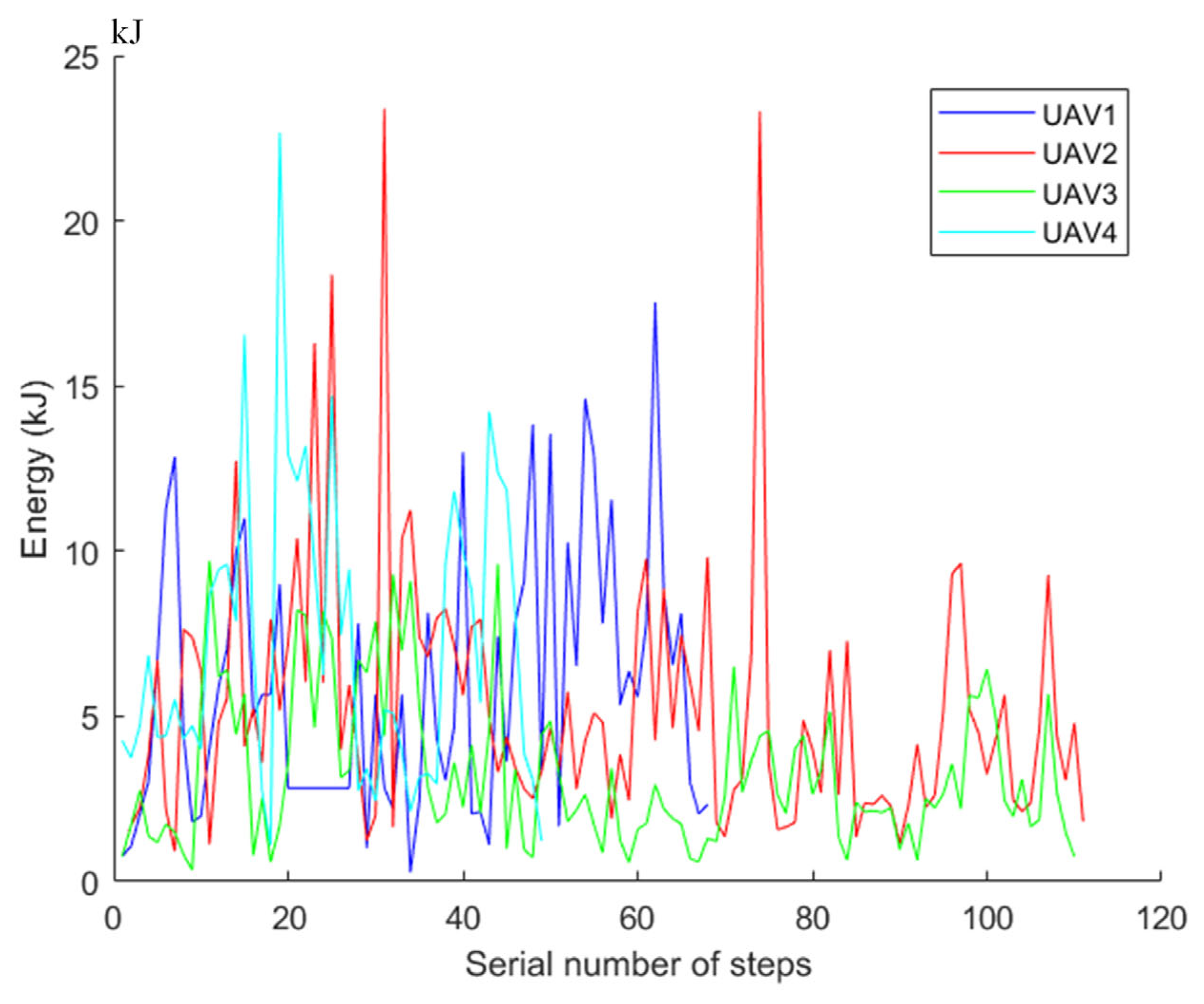
Figure 12 demonstrate that the MNRW-LSA algorithm outperforms other algorithms in terms of optimal solution value under the same number of iterations and population size. Specifically, the optimal solution value of MNRW-LSA is 91.75, which is significantly better than the optimal solution values of standard PSO (120.39), standard SA (136.13), and standard LSA (140.52). These findings suggest that the MNRW-LSA algorithm is not only faster but also more accurate in terms of convergence speed and accuracy compared with the other algorithms. The energy loss of each node of the four UAVs is shown in
Figure 13.
In algorithm analysis, the total number of executions of the statement is a function of the problem size , and then the change of when is analyzed, and the order of magnitude of is determined. The time complexity of the algorithm, which is the time measure of the algorithm, is denoted as . It means that with the increase of the problem size n, the length rate of the algorithm execution time is the same as the length rate of , which is called the asymptotic time complexity of the algorithm, referred to as time complexity, where is some function of the problem gauge . According to the order in which the time complexity is arranged , when n approaches infinity, only the terms of higher order are retained so that the time complexity results obtained by the analysis are more efficient and reliable. The time complexity of the MNRW-LSA algorithm is , and the time complexity of the LSA algorithm is , where is the population dimension and is the number of duplicate channels.
In the MNRW-LSA algorithm, the loss of a more efficient discharge channel is prevented due to the improved method, which makes it more efficient to find an efficient channel. At the same time, the random walk strategy enables the algorithm to avoid repeated path optimization, which improves the overall optimization efficiency of the algorithm. Therefore, the algorithm should have a shorter run time and higher optimization efficiency than the LSA algorithm.
According to the data in
Table 8, in running the three algorithms 30 times, the results of the algorithm proposed in this paper are all the best from the perspective of any of the three indicators: the optimal solution, the worst solution, and the average value. The paper presents an improved version of the MNRW-LSA algorithm that shows higher convergence accuracy and faster speed in solving the problem of simultaneous urban patrol path optimization by multiple UAVs. The algorithm also exhibits strong robustness and uniformity, making it a promising approach for this task.
At the same time, the optimal path length obtained by the MNRW-LSA algorithm is shortened by 305.46 m at most and 124.66 m at least. Compared with other algorithms, the optimal coverage rate has increased by 11.78% at most, reaching 86.20%, indicating that the path is well planned, and most of the building groups and other spaces can be observed.
However, the average running time of the MNRW-LSA algorithm is longer than that of the PSO and SA algorithms. After analyzing the process and principle of each algorithm, we have identified that the MNRW-LSA algorithm takes longer to run due to the inclusion of the cross-fetching process. This process is repeated in each iteration to ensure the accuracy of the results, resulting in a running time that is approximately 1 s longer than other algorithms. However, compared with the basic LSA algorithm, the number of times the channel time is reset to zero is reduced due to the multi-level nesting process, which significantly speeds up the running time.
6. Conclusions and Future Research
This paper explores the patrolling of multi-UAVs in urban environments and the optimization of their trajectories. A three-dimensional topographic map was created for certain building areas in Beijing, China, to support this research. The study takes into account the UAV’s three-dimensional flight constraints, performance constraints, and terrain constraints to establish a path cost model for multiple UAVs to patrol together.
To optimize the UAV trajectory cost in the model, we have enhanced the classical RRT algorithm by incorporating a greedy strategy inspired by optimization algorithms. This has led to the development of the GP-RRT algorithm, which effectively generates an initial path for path arrangement. Our focus is on achieving both extensive patrol coverage and a short path during UAV path planning. The patrol direction of the UAV is partitioned into larger areas so that there is no overlapping of UAV patrol areas as far as possible.
This paper proposes the use of a multi-layer nesting strategy and random tour strategy to enhance the performance of the lightning search algorithm. The resulting algorithm, MNRW-LSA, is then compared to other algorithms, such as PSO, SA, and LSA. The study shows that MNRW-LSA outperforms these other algorithms. The results show that the MNRW-LSA algorithm optimizes the path length to 1497.03 m and achieves a coverage rate of 86.20%. Its convergence speed and convergence accuracy are significantly higher than other algorithms. The algorithm effectively optimizes the UAV’s trajectory in urban patrols and proves the correctness of the model. It has great advantages in solving the Multi-UAV trajectory planning problem.
The starting point of a UAV changes based on real-time data obtained from the road detection system, such as navigation. This allows a UAV to adapt to changes in vehicle and population density, completing its work in a real-time environment. The contributions of the paper are summarized as follows.
This manuscript introduces the concept of UAV urban patrol, which addresses the need for efficient surveillance and monitoring in urban environments. Furthermore, a reality-based model of the urban environment is developed, providing a realistic representation for evaluating the proposed solutions.
In order to address the challenges of UAV urban patrol effectively, the mathematical model has been expanded to consider various factors. These include the impact cost of UAV operations, flight energy consumption cost, and mission execution rate. Moreover, the model takes into account the constraints imposed by the UAV’s flight range and range limitation, resulting in a comprehensive approach to optimizing UAV patrol strategies.
A novel approach called the multi-level nesting and random walk strategy (MNRW-LSA) has been developed to enhance the performance of the lightning search algorithm (LSA) and achieve better resource allocation optimization. The MNRW-LSA algorithm incorporates multiple levels of nesting and employs a random walk strategy to improve search efficiency and accuracy, enabling more effective allocation of resources for UAV urban patrol.
The reliability and integrity of the MNRW-LSA model are validated through simulation experiments. These experiments demonstrate the effectiveness of the proposed algorithm in comparison to other existing algorithms commonly used in UAV urban patrol scenarios. The comparison provides valuable insights into the superior performance and benefits of the MNRW-LSA approach.
This paper provides a new improvement idea for UAV path planning, which can effectively solve the related planning problems in static path planning. However, there are still limitations in the current research process. For example, the interference of weather factors during UAV flight and the changes in vehicle and population density in the real-time environment are not considered. In future research, more improvement strategies should be tried to be introduced, which will better improve the algorithm performance. At the same time, we will consider applying machine learning methods to learn and optimize the search strategies of heuristic algorithms to improve the efficiency of solving and the quality of solutions, thereby addressing more complex task environments.


