Design and Implementation of UAV Velocity Controller Based on Reference Model Sliding Mode Control

Abstract

In recent years, multi-rotor unmanned aerial vehicles (UAV) have been widely applied for various applications; however, they are yet to be as commonly utilized in certain industrial transportation applications. Thus, this work designed and implemented a reference model-based integral sliding mode control (SMC) method applied to the velocity controller of a multi-rotor UAV. The designed controller was compared with an integral SMC scheme, and then the controller and modeling robustness were verified. Finally, the proposed method was applied to an industrial six-rotor UAV. Three experiments involving target-tracking, fixed-point hovering, and robustness verification were executed. A load of approximately 81.5% of the UAV’s self-weight was used to verify the robustness of the proposed scheme against parameter uncertainty. This work will serve as a meaningful reference for the application of the SMC in practical industrial applications.

1. Introduction

With the increase in the popularity and adoption of unmanned aerial vehicles (UAVs), many successful cases have emerged that show that the application of UAV technology can effectively solve problems in traditional production applications. A mere simple flight cannot meet the demands of today’s society. Instead, modern applications that require capabilities such as carrying different types of equipment, autonomous flight in different environments, and performing specific tasks are more attractive; these include applications such as logistics and transportation [1], plant protection [2], and power inspection [3]. The application of UAVs relies on trajectory planning and target tracking. Trajectory planning helps calculate a safe and optimal path in the environment, and the controller ensures that the UAV flies along the planned route. Therefore, a well-designed controller that is accurate and robust against parameter uncertainty is critical.

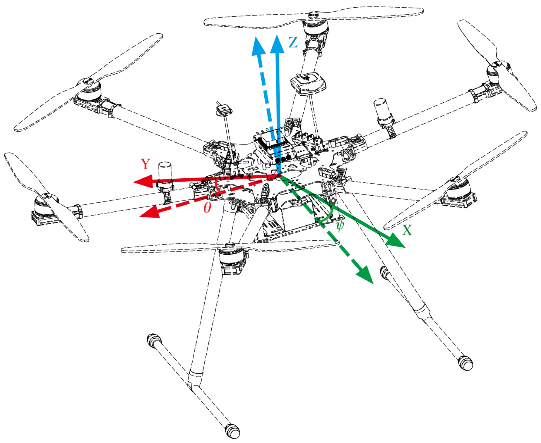
A classic multi-rotor UAV is a typical underactuated system that has the characteristics of being nonlinear and robust coupling [4]. During flight, there will be interference from the environment, such as wind, air pressure, and humidity changes. In addition, carrying different equipment during various tasks is essential, which introduces uncertainty in parameters. Due to the underactuated characteristic, the control system design usually adopts a cascaded structure. Heading control is usually considered separately due to the differential flat property [5]. After extensive research and development, in addition to proportional–integral–derivative control (PID) [6,7], various schemes have also been proposed to improve the flight stability and robustness, such as active disturbance rejection control [8], intelligent control [9], robust control [10], and sliding mode control (SMC) [11].

SMC is an effective technique to deal with complex nonlinear systems with uncertainties and disturbances [12,13]. It has been widely used in UAV controller design due to its fast response and anti-disturbance ability [14,15,16,17,18,19]. Regarding the position and attitude control, Noordin et al. proposed a sliding mode adaptive PID controller applied to a micro air vehicle (MAV) with a mass less than 0.1 kg [20]. A model-free SMC design has also been realized; Precup et al. proposed two model-free SMC design schemes [21], while Abro et al. proposed a model-free SMC combined with fuzzy strategies [22]. To cope with sensor noise and random disturbance, Jing et al. designed a nonlinear SMC connected with a disturbance observer and verified it in the PX4 simulation environment [23]. In [24], the model uncertainty and disturbance were considered. Maurya et al. used fractional-order SMC to design the attitude and position controller; they verified its effectiveness with a hovering and trajectory tracking simulation. However, the aerodynamic effect was not included in the simulated environment because it is unknown; moreover, the scheme is yet to be verified for actual flight.

Ríos et al. proposed a tracking strategy consisting of a finite-time sliding mode observer, a PID controller, and a continuous sliding mode controller. The author focused on the position and attitude control and verified the effectiveness via trajectory tracking experiments [25]. Regarding attitude control, Derafa et al. designed and implemented a second-order sliding mode technology that is robust against bounded external disturbances and is based on the super-twisting algorithm [26]. Muñoz et al. proposed an improved super-twisted sliding mode controller for altitude control. They compared it with three second-order SMC methods in a simulated as well as an actual environment, and the experiments showed that the enhanced scheme is robust against disturbances [27]. Although the aforementioned techniques have proven effective in real-world UAV systems, their impact on parameter uncertainty has yet to be validated.

In [28], Mu et al. proposed an integral synovial film control to realize the waypoint flight of a UAV under model uncertainty and external disturbance. During the experiment, a weight of 0.17 kg (12.1% of the UAV weight) was considered as the parameter uncertainty. After increasing the 0.17 kg payload, the mean square error of its tracking error increased by 14.5%. Similarly, Wang et al. proposed a non-cascade adaptive SMC trajectory tracking control. In the verification process, loads equivalent to 10% (0.1 kg) and 20% (0.2 kg) of the UAV self-weight were used as the uncertain parameters [29]. An increase of 0.2 kg in the payload resulted in a significant decline in the X-Y plane tracking performance of the UAV. Further payload additions can alter the dynamics of the drone, particularly if the weight distribution shifts drastically. This change in dynamics can result in a decrease in the controller performance, as confirmed by the experiments in references [28,29]. To the best of our knowledge, researchers are yet to find any solutions and applications related to multi-rotor UAVs that can accommodate high payloads (more than 50% of a UAV’s self-weight) without sacrificing the flight performance, which are useful in industrial applications. There are some commercial drones that can tolerate large payload changes [30], but their flight data and control systems have not been published yet, and it is unknown how well they can maintain their flight performance in the face of payload changes.

With the aim of developing a velocity control method for UAVs that is robust against parameter uncertainty, we implemented and tested a reference model integral SMC scheme [31] based on a data-driven model. Our approach, distinct from previous studies [19] that relied on accurate dynamic models, utilized flight data to derive the data-driven model. The results of our simulations and experiments demonstrate the effectiveness of our method. Our work has three main contributions:

• By focusing on parameter uncertainty, we implemented and verified an integral sliding mode velocity control scheme based on a reference model that can maintain stability, even with significant changes in parameters;
• The complete design process is explained. Based on the steps provided herein, the proposed method can be easily implemented in various UAV systems and controllers; thus, it is not limited to the velocity controller;
• The robustness of our model to errors was confirmed through a large number of simulations and flight tests. We altered the verification and controller design models to verify their robustness and compared the results with an LQR-based integral SMC scheme in simulations. The target-tracking, hovering, and robustness verification experiments were then conducted on a six-rotor UAV. The robustness verification results indicate that the proposed scheme can accommodate up to 81.5% of a payload change without compromising the tracking performance.

The rest of this paper is organized as follows: We analyze and deduce the velocity dynamic motion in Section 2. Section 3 details the components of the proposed method. In Section 4, the detailed design process is shown, and then the designed controller is used for the simulation and actual flight verification. The conclusions and future plans are discussed in Section 5.

2. Problem Formulation

2.1. Velocity Tracking Control

Before the actual analysis, a brief introduction to the structure of a UAV control system will be helpful. Due to the underactuated characteristic, a form of multi-stage series is usually adopted in the control system design. For PX4, a classic open-source system, the control system can be categorized under four parts: position control, attitude control, stabilize control, and motor output. It is worth noting that the position controller in PX4 contains two components: velocity target calculation and attitude target calculation. This work is aimed at the latter.

The velocity controller relies on a well-designed closed-loop attitude system, which means that the attitude system is included in the design process. The target velocity is the controller’s input, which can be obtained from the velocity target calculation in the position controller or the ground station command.

2.2. Velocity Dynamics

The movement of a multi-rotor UAV relies on the rotation speed of each rotor and propeller. It can maintain different attitudes to realize movement by adjusting the lift force. During horizontal flight movement, the fuselage will remain tilted, as shown in Figure 1.

Implementing the mechanical analysis of the UAV in the tilted position, the vertical component of the lift cancels the gravity, whereas the horizontal portion cancels the air resistance to provide power for the movement. Neglecting kinematic coupling and assuming that the attitude is within a small range (±0.5 rad) [22], the dynamic of the UAV can be expressed as

$$ma=mg\theta -C_v{v}^2,$$

(1)

where m is the mass, a represents the dynamic acceleration, g denotes gravity, $\theta$ is the attitude corresponding to the movement, $C_v$ is the air resistance, and v denotes the real-time velocity. Coefficient $C_v$ will be affected by factors such as the movement velocity, the rotating acreage of propellers, and the tilt angle. For simplicity, it can be assumed to be constant. Thus, Equation (2) can be derived from obtained (1):

$$\dot{a}=g\dot{\theta }-\frac{2C_v}{m}v$$

(2)

As discussed in Section 2.1, the attitude system is included in the velocity dynamic. In the case where the target attitude can be accurately tracked, and consequently the attitude closed loop can be simplified as a standard first-order inertial system, the relationship between target attitude ${\theta }_r$ and the real-time attitude $\theta$ can be established as:

$$\dot{\theta }=\frac{K_{Att}{\theta }_r-\theta }{T_{Att}}.$$

(3)

$K_{Att}$ and $T_{Att}$ are the parameters of the first-order inertial system. Combining Equations (2) and (3), the velocity dynamic can be expressed as

$$\dot{a}=-\frac{g}{T_{Att}}\theta -\frac{2C_v}{m}v+\frac{g{K}_{Att}}{T_{Att}}{\theta }_r.$$

(4)

In addition, the measured result (the velocity with time delay) of the velocity sensor has an inherent time delay $t_d$; thus, it can be considered as the extended state. Selecting attitude $\theta$, dynamic acceleration a, real-time velocity v, and delayed velocity $v_d$ as system states X, and using target attitude ${\theta }_r$ as the system input u, Equation (4) can be rewritten as:

$$\left\{\begin{array}{c}\dot{X}=AX+Bu,\hfill \\ Y=CX,\hfill \end{array}\right.$$

(5)

among them,

$$A=\left[\begin{array}{cccc}-\frac{1}{T_{Att}}& 0& 0& 0\\ -\frac{g}{T_{Att}}& -\frac{2C_v}{m}& 0& 0\\ 0& 1& 0& 0\\ 0& 0& \frac{1}{t_d}& \frac{1}{t_d}\end{array}\right], B=\left[\begin{array}{c}\frac{K_{Att}}{T_{Att}}\\ g\frac{K_{Att}}{T_{Att}}\\ 0\\ 0\end{array}\right], C=\left[\begin{array}{cccc}1& 0& 0& 0\\ 0& 0& 0& 1\end{array}\right],$$

(6)

where $t_d$ depends on the velocity measurement sensor.

3. Velocity Controller Design

3.1. Proposed Method Structure

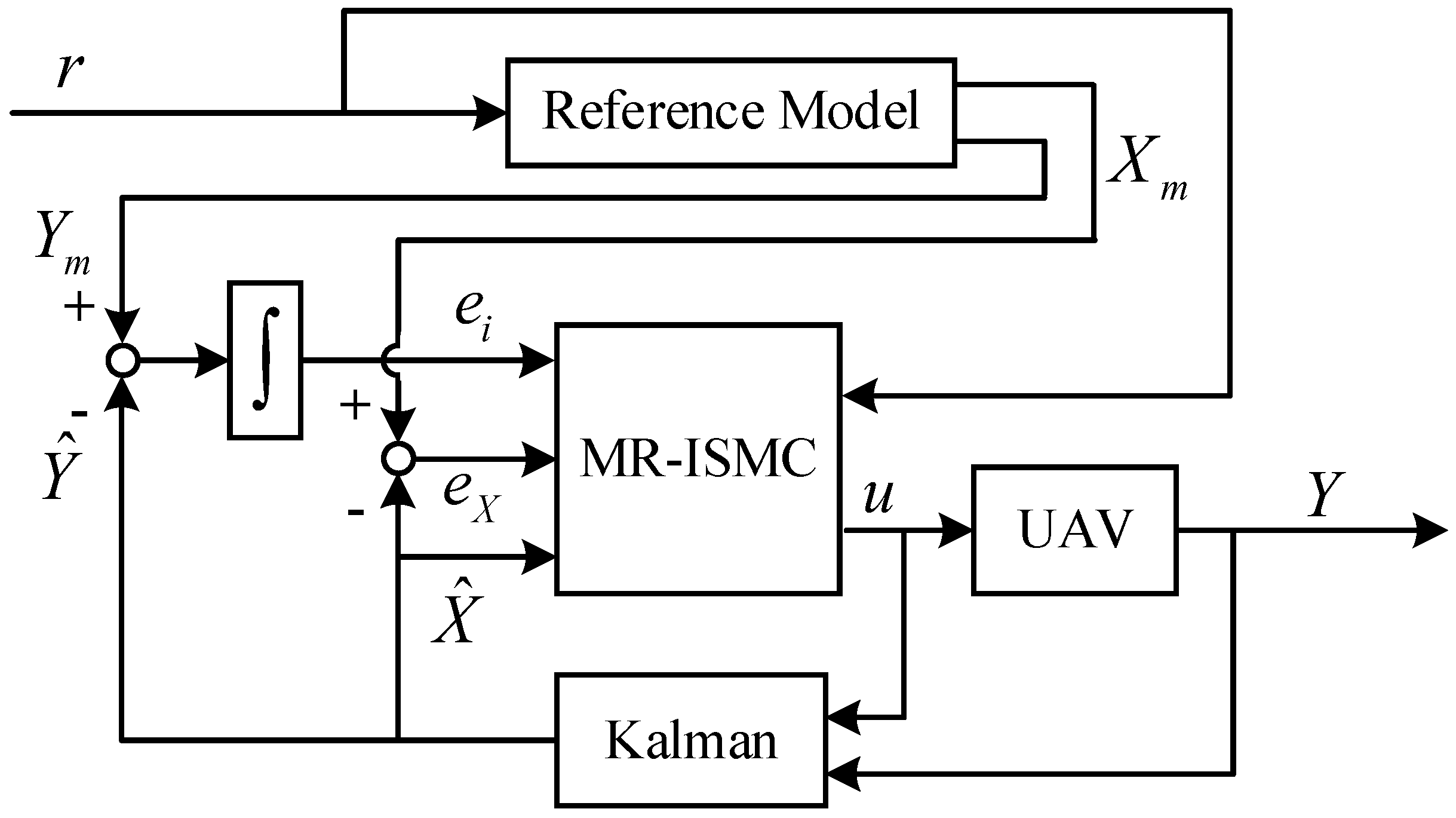
The structure of the proposed method is shown in Figure 2. It consists of a Kalman filter, reference model, and sliding mode controller.

The Kalman filter is used to filter sensor data and estimate dynamic acceleration, which is difficult to measure directly. The design of the reference model can effectively avoid any abrupt target change. It can also calculate the target change rate, and the change rate can be considered the target of the dynamic acceleration. Finally, the obtained information and the integral of the system error are used to design the controller, and the controller output is used as the attitude target.

The specific design process of each component is described below.

3.2. State Estimator

Most feedback states can be measured directly, except dynamic acceleration. UAVs inevitably vibrate during flight, which becomes more evident as their size increases. This problem is unavoidable in industrial applications. Therefore, a method capable of estimating unknown states and filtering the original sensor data is required. A steady-state Kalman filter was selected for this task.

The steady-state Kalman filter can be regarded as a multi-input linear system, where the estimation result is composed of multiple input data. The contribution of a single input data to the final estimation result can be calculated independently [32]. Considering the dynamics (Equation (5)) of Gaussian noise w on the input and the output measurement noise v, the discrete system can be described as:

$$\left\{\begin{array}{c}{X}_d(t+1)=\Phi X_d\left(t\right)+\Gamma u\left(t\right)+\Gamma w\left(t\right),\\ Y_d\left(t\right)=H{X}_d\left(t\right)+v\left(t\right).\end{array}\right.$$

(7)

The steady-state Kalman filter was designed according to Equation (7), and its state update and measurement update processes are shown in Equations (8) and (9), respectively.

$${\widehat{X}}_d(t+1|t)=\Phi {\widehat{X}}_d\left(t\right|t-1)+\Gamma u\left(t\right),$$

(8)

$$\begin{array}{c}{\widehat{X}}_d\left(t\right|t)={\widehat{X}}_d\left(t\right|t-1)+M({\widehat{Y}}_d\left(t\right)-H{\widehat{X}}_d\left(t\right|t-1)),\\ {\widehat{Y}}_d\left(t\right|t)=H{\widehat{X}}_d\left(t\right|t),\end{array}$$

(9)

where M is the optimal innovation gain and is used to minimize the estimation error under the noise covariance $Q=E(w(t)w{(t)}^T)$ and $R=E(v(t)v{(t)}^T)$. Under ideal conditions, the error-free estimation of X can be realized. Thus, we assumed that $\widehat{X}=X$ holds in the controller design process.

3.3. Reference Model

The SMC method calculates a large output to ensure robustness when facing harsh targets. However, in the UAV velocity control system, a larger output translates to a larger attitude target, which can be dangerous, especially in industrial applications. Thus, a reference model is used by arranging the transition process to avoid harsh targets.

Similar to Equation (5), the reference model can be designed as:

$$\left\{\begin{array}{c}{\dot{X}}_m=A_m{X}_m+B_{m}r,\hfill \\ Y_m=C_m{X}_m.\hfill \end{array}\right.$$

(10)

The original velocity target r is the input of the reference model system, state $X_m=\left[\begin{array}{ccc}{\theta }_m& a_m& v_m\end{array}\right]$ corresponds to X. The delayed velocity $v_d$ is not considered in Equation (10) because the main function of $v_d$ is to verify the estimator. The input matrix $B_m$ is related to B and satisfies $B_m=B_{3\times 1}{K}_1$, $B_{3\times 1}$, which represents the sub-matrix of the first three rows and the first column in B. While the sub-matrixes of state space $A_m$ and A have the same structure, $C_m$ is similar to the sub-matrix of C:

$$A_m=\left[\begin{array}{ccc}{k}_{m0}& 0& 0\\ k_{m1}& k_{m2}& k_{m3}\\ 0& 1& 0\end{array}\right],C_m=\left[\begin{array}{ccc}0& 0& 1\end{array}\right].$$

(11)

In Equation (11), $k_{m0}$, $k_{m1}$, $k_{m2}$, and $k_{m3}$ are negative constants, which can be obtained through debugging and satisfy the constraints

$$B_{3\times 1}{K}_2=A_m-A_{3\times 3}.$$

(12)

For the original target r, the reference model output will catch up to the target within a limited time. This means that the system output $Y_m$ will be consistent with the input r, and that $X_m$ will not change when the time tends to infinity, which means that ${\dot{X}}_m=0$, $Y_m=r$. Combining this with the reference model, Equation (13) can be obtained.

$$C_m{A}_m^{-1}{B}_{m}r=C_m{A}_m^{-1}{B}_{3\times 1}{K}_{1}r=r$$

(13)

Then, $K_1=-{\left(C_m{A}_m^{-1}{B}_{3\times 1}\right)}^{-1}$ can be obtained, and the input matrix of the reference model can also be expressed as:

$$B_m=-B_{3\times 1}{\left(C_m{A}_m^{-1}{B}_{3\times 1}\right)}^{-1}.$$

(14)

The above process shows that $B_m$ can be obtained by $A_m$, and $C_m$ in the reference model is similar to the output matrix in Equation (5). Therefore, the concrete effect of the reference model can be tuned by choosing appropriate parameters for $k_{m0}$, $k_{m1}$, $k_{m2}$, and $k_{m3}$.

3.4. Integral Sliding Mode Control

After the state estimator and the reference model were designed, the SMC was used to design the velocity controller of the UAV. In this regard, the feedback state $X=\widehat{X}$ is assumed, and the error between the feedback state and the reference state $X_m$ is $e_X=X_m-X_{3\times 1}$; then, the derivative of the error is

$${\dot{e}}_X=A_m{e}_X+(A_m-A_{3\times 3})X_{3\times 1}+B_{3\times 1}u-B_{m}r.$$

(15)

According to the constraints of Equation (12), Equation (15) can be simplified as

$$\begin{array}{c}{\dot{e}}_X=A_m{e}_X+B_{3\times 1}{u}_s,\hfill \\ u_s=-(K_2{X}_{3\times 1}+K_{1}r-u).\hfill \end{array}$$

(16)

To further improve the target-tracking accuracy and stability, the velocity tracking error integral $e_i$ is considered as an extended state to the error dynamics. The extended error system is expressed in Equation (17):

$$\begin{gathered} {\dot{e}}_s=\left[\begin{array}{c}{\dot{e}}_X\\ {\dot{e}}_i\end{array}\right]=\left[\begin{array}{cc}{A}_m& 0\\ C_m& 0\end{array}\right]\left[\begin{array}{c}{e}_X\\ e_i\end{array}\right]+\left[\begin{array}{c}{B}_{3\times 1}\\ 0\end{array}\right]u_s \\ =A_s{e}_s+B_s{u}_s \end{gathered}$$

(17)

The sliding surface $\sigma$ is represented by Equation (18), and its derivative is included in Equation (19):

$$\sigma =S{e}_s,$$

(18)

$$\dot{\sigma }=S{A}_s{e}_s-S{B}_s(K_{1}r+K_2{X}_{3\times 1}-u),$$

(19)

where $S=\left[\begin{array}{cccc}{k}_{s0}& k_{s1}& k_{s2}& k_{s3}\end{array}\right]$ is the parameter corresponding to $e_s$. When the state variable converges to the sliding surface, the equivalent input $u_{eq}$ can be calculated.

$$u_{eq}=-{\left(S{B}_s\right)}^{-1}S{A}_s{e}_s+K_{1}x+K_{2}r$$

(20)

The smooth function (21) is used to replace the sign function in the traditional SMC method to suppress chattering.

$$f\left(\sigma \right)=\frac{\sigma }{\left|\sigma \right|+\delta },$$

(21)

where $\delta$ is a relatively small positive number; then, $u_{sw}$ can be represented as

$$u_{sw}=K_{n}f\left(\sigma \right).$$

(22)

$K_n=-c{\left(S{B}_s\right)}^{-1}$ is the gain coefficient and $c>0$ in $K_n$ is the adjustable gain. The final output of the proposed reference model-based integral SMC is

$$u=u_{eq}+u_{sw}.$$

(23)

To verify the stability of the control output (23), the Lyapunov function can be defined as

$$V=\frac{1}{2}{\sigma }^2.$$

(24)

The time derivative of Equation (24) is $\dot{V}=\sigma \dot{\sigma }$; combining Equations (19)–(23), the derivative form can be expanded as

$$\begin{array}{cc}\hfill \dot{V}& =\sigma \dot{\sigma }\hfill \\ \hfill & =\sigma \left[S(-B_s{K}_{2}X+A_s{e}_s+B_{s}u-B_s{K}_{1}r)\right]\hfill \\ \hfill & =\sigma [-S{B}_s{K}_{2}X+S{A}_s{e}_s+S{B}_s(K_{2}X+K_{1}r-{\left(S{B}_s\right)}^{-1}S{A}_s{e}_s+K_{n}f\left(\sigma \right))-S{B}_s{K}_{1}r]\hfill \\ \hfill & =\sigma [-S{B}_s{K}_{2}X+S{A}_s{e}_s+S{B}_s{K}_{2}X+S{B}_s{K}_{1}r-S{B}_s{\left(S{B}_s\right)}^{-1}S{A}_s{e}_s+S{B}_s{K}_{n}f\left(\sigma \right)-\hfill \\ \hfill & S{B}_s{K}_{1}r]\hfill \\ \hfill & =\sigma \left[S{B}_s{K}_{n}f\left(\sigma \right)\right]\hfill \\ \hfill & =\sigma \left[S{B}_s-c{\left(S{B}_s\right)}^{-1}f\left(\sigma \right)\right]\hfill \\ \hfill & =-c\sigma f\left(\sigma \right)\hfill \end{array}$$

(25)

Because $\sigma f\left(\sigma \right)⩾0$ and $c>0$, the conclusion $\dot{V}⩽0$ can be drawn; thus, when $\dot{V}\equiv 0$, $\sigma \equiv 0$, according to LaSalle’s invariance principle, the proposed controller is asymptotically stable.

The design process of the proposed method can be summarized as follows:

Step 1.

Obtain the model first. Collect the flight data to fit the system model.

Step 2.

The next step involves designing the state estimator. Set the covariance matrix and implement the state estimator.

Step 3.

Then, design the reference model. Tune the parameters to adjust $A_m$, and then design the reference model using Equations (11) and (14).

Step 4.

Finally, implement the controller. Select the parameters S, c, and $\delta$, and then the controller can be designed according to Equations (20), (22), and (23) by combining the data of the fitted model and the reference model.

4. Simulation and Experiment

4.1. Experiment Platform

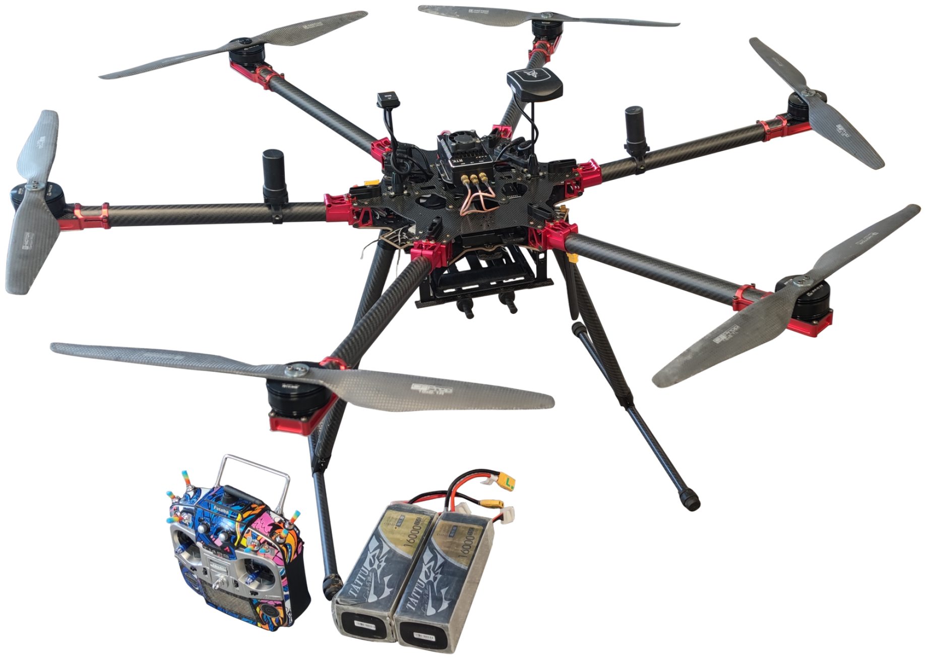
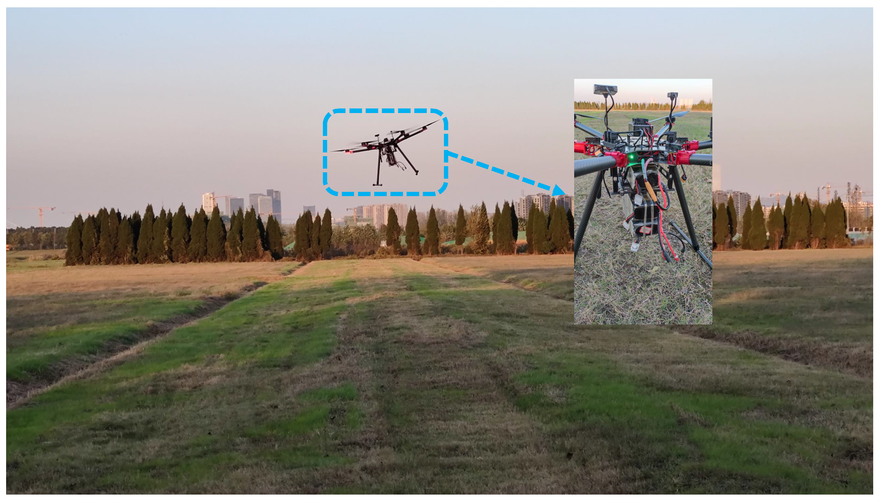
The proposed scheme was established in a six-rotor UAV with a wheelbase of 960 mm for verification, as shown in Figure 3.

The UAV was established using an open-source frame, and the flight control system used was developed by our laboratory, including the IMU modules, GNSS modules, MAG modules, data recording module, power module, LED, and central module. The central module was designed based on STM32F4, while the flight control system structure was implemented based on PX4. In addition, we installed a real-time differential positioning device (RTK) on the UAV to obtain a high-precision real-time velocity and position.

4.2. RM-ISMC Design Process

This section will describe the design process of our method in detail, taking the velocity controller in the Y-axis direction as an example.

Step 1.

Obtain the model first.

The data-driven models can be obtained by fitting the flight data. For this, the Y-axis velocity measured by the GNSS sensor, roll, and roll target is necessary. In the Ident-Box of MATLAB, the feedback and target of the roll are used to fit the attitude closed-loop system; subsequently, $K_{Att}$ and $T_{Att}$ can be obtained.

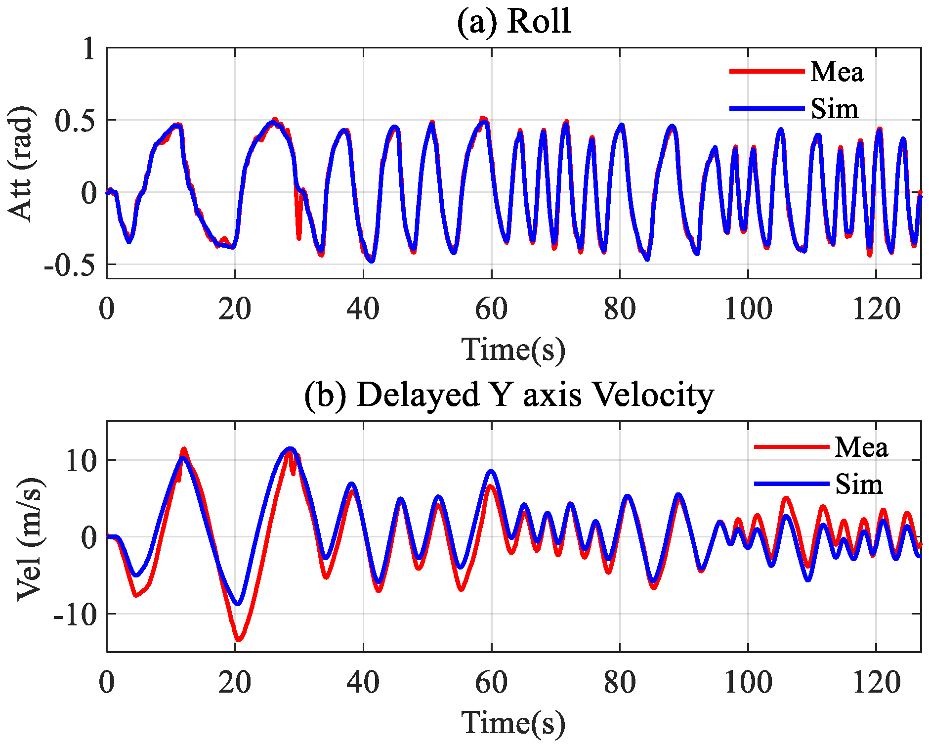
After the attitude closed-loop system is obtained, $C_v$ can be obtained via debugging. The parameter $C_v$ can be adjusted by comparing the delayed velocity of the simulation output with the measured value. The final simulation model output is shown in Figure 4, and the specific values of each parameter are shown in

Table 1. Velocity model parameters.

Parameter	Value	Unit
m	5.96	kg
g	9.81	N/kg
$K_{Att}$	0.93	-
$T_{Att}$	0.27	-
$C_v$	0.01	-
$t_d$	0.2	second

.

In Figure 4a, the red line is the measured value during the flight, while the blue line is the simulation output of the fitting model; under the same roll target, the fitting model output is consistent with the roll during flight. However, there are certain deviations in the delayed velocity, as shown in Figure 4b. The primary reason for this is that $C_v$ is obtained by tuning, and the slight model deviation can be ignored, which will be verified later. The parameters in Table 1 can be considered to characterize the velocity model (Equation (5)).

Step 2.

Designing the state estimator.

The noise covariance was selected as Q = 0.1, R = [0.1, 10], and combining the fitted velocity model, the steady-state Kalman filter was established. The target attitude, attitude, and velocity were selected as the inputs. This process was implemented using the Kalman function in MATLAB.

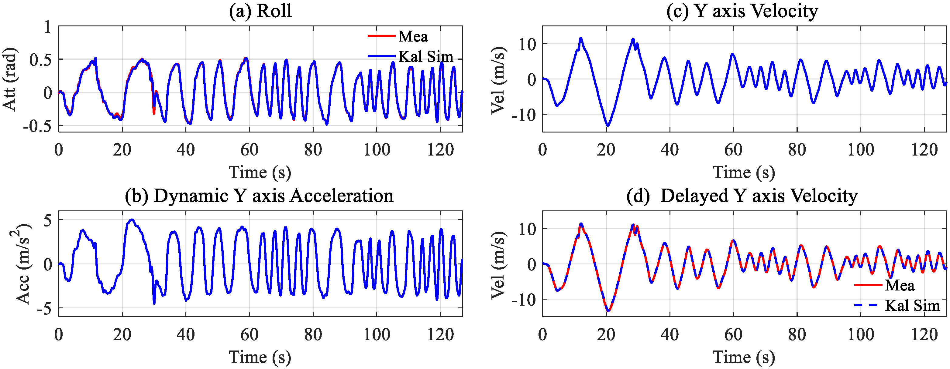
Figure 5 shows the estimated results, where Figure 5b,c show the dynamic acceleration and velocity changing under the input. The red lines in Figure 5a,d represent the measured roll and velocity, respectively, and the estimated results coincide exactly with the measured data. Therefore, the estimated dynamic acceleration and the real-time velocity are completely trustworthy.

Step 3.

Design the reference model.

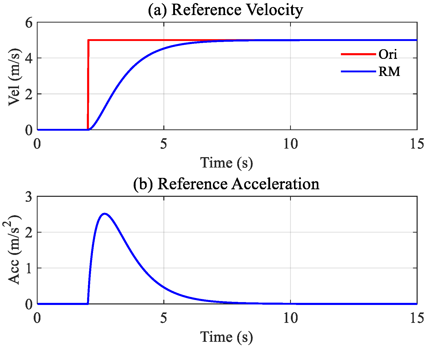
The parameters used in the reference model are tuned to $k_{m0}=15$, $k_{m1}=40$, $k_{m2}=3$, and $k_{m3}=2$; then, $B_m$ can be calculated. Taking a step signal of 5 m/s as an example, the output of the reference model is shown in Figure 6.

The red line in Figure 6a is the original target velocity and the blue curve is the processed reference velocity; the acceleration reference shown in Figure 6b is also planned simultaneously. The transition process can be completed within 6 s. The specific tracking time can be adjusted by changing the parameters in $A_m$.

Step 4.

Implement the controller.

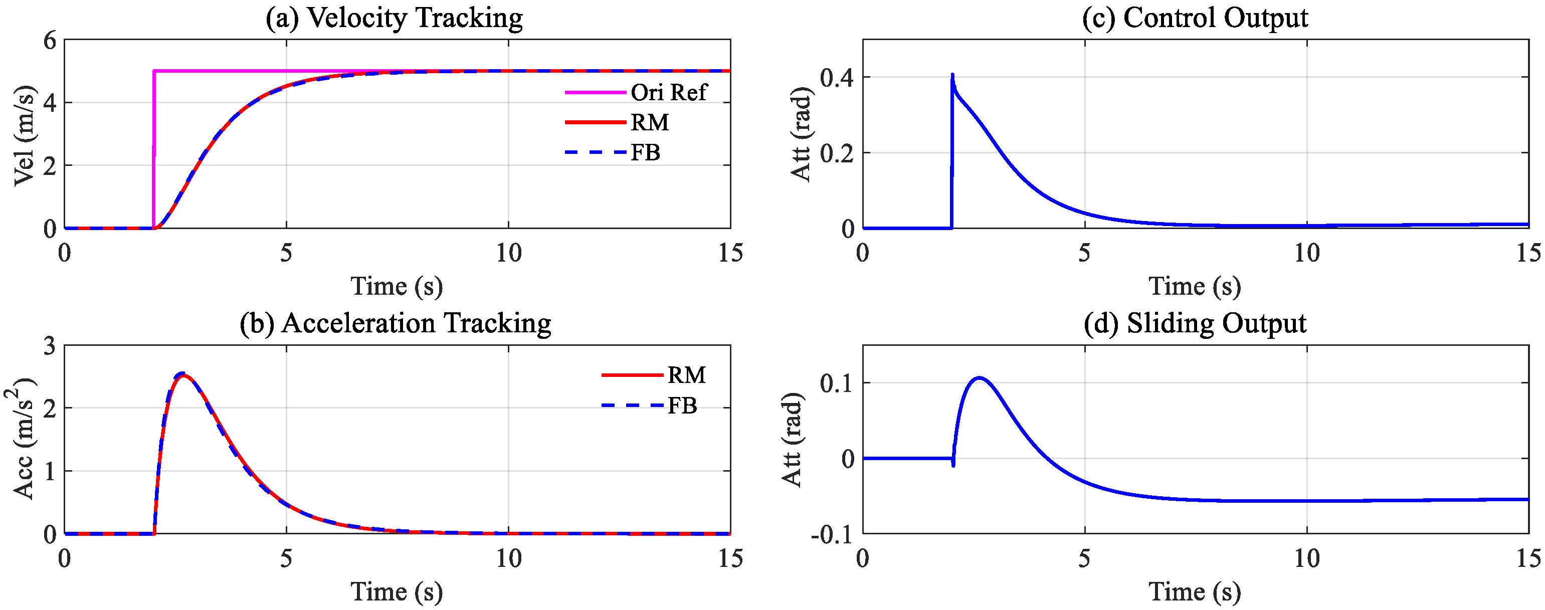
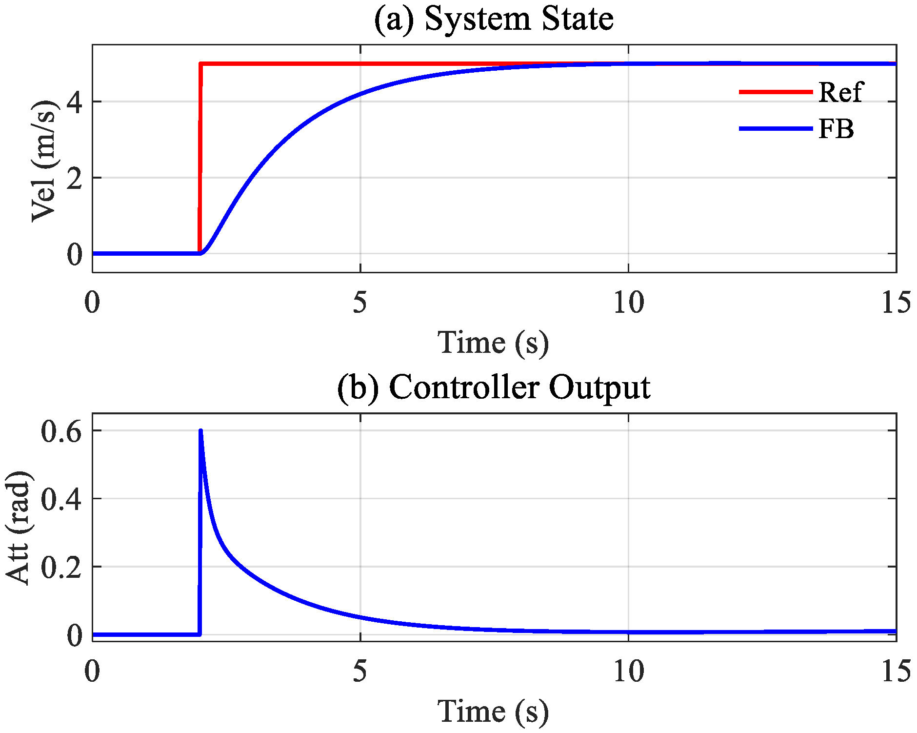
For the mathematical model (5), $c=1.6$, $\delta =0.2$, and $S=$ [−0.5268, 0.3255, 0.9954, 0.5511] are the tunable parameters, and the performance for tracking the 5 m/s step is proposed in Figure 7.

From Figure 7a,b, the velocity and acceleration can adequately track the relevant target, and the tracking process is completed within 6 s, which is consistent with the reference model simulation results. From Figure 7c, it can be seen that the maximum controller output is 0.4 rad, which is within the assumed safe range. In addition, there is no chattering in the process.

4.3. Simulation Validation

To verify the effectiveness of the proposed method, we compared it with a similar robust control scheme. The scheme in [28] demonstrated that it can accommodate a 10% parameter variation in its weight with a small 1.4 kg UAV. Considering the system $\dot{X}=AX+B\theta$, the designed controller can be expressed as

$$u_{\theta }=u_o+u_n.$$

(26)

Among them, $u_o=-FX$ is obtained through the LQR method mentioned in [33], $u_n=-\rho {\left(GB\right)}^{-1}\frac{{\sigma }_r}{∥{\sigma }_r∥}$, $G={\left(B^{T}B\right)}^{-1}{B}^T$ is related to the model, $E=X-\overline{X}$ is the error between the system state and the target state $\overline{X}$, and $\rho >0$ is the modulation gain. ${\sigma }_r$ is the designed sliding manifold, and its specific form is

$${\sigma }_r=GE-G{E}_0-G{\int }_0^t(AE\left(\tau \right)+B{u}_o\left(\tau \right))d\left(\tau \right).$$

(27)

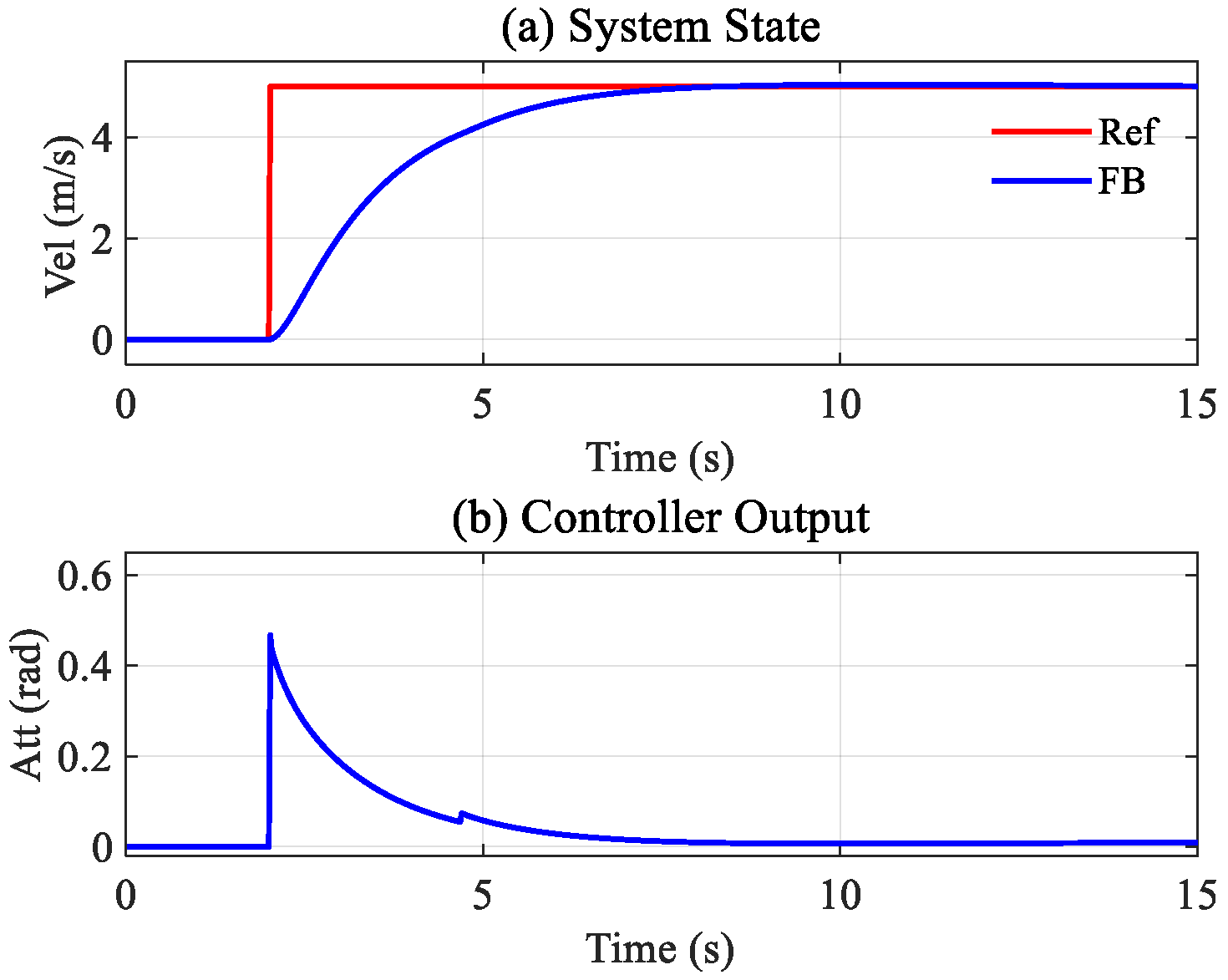
We designed the controller of the system (Equation (5)) according to Equation (26) and set the adjustable parameter $\rho =0.01$. During the LQR design process, the weight in the cost function was $R_l=120$, and $Q_l$ was a diagonal matrix, with eigenvalues $[0.5,0.5,1]$. Taking a step signal of 5 m/s as the target, the tracking effect is shown in Figure 8.

In Figure 8b, a small chatter is induced by the switching function in the sliding mode algorithm. Nevertheless, the comparison scheme maintains a satisfying tracking performance under the tuned parameters.

At the same time, a set of well-tuned PID schemes was also considered for the comparison, and the parameters were adjusted based on Equation (5). The final tracking effect is shown in Figure 9.

The tracking results in Figure 8 and Figure 9 show that the two contrast schemes can track the target signal accurately under the adjusted parameters. The contrast and proposed schemes’ parameters are summarized in

Table 2. Controller parameters of the three methods.

Method	Derived Parameter	Tunable Parameter
A. PID	-	$\begin{array}{c}{K}_p=-0.12\hfill \\ K_i=-0.001\hfill \\ K_d=-0.1\hfill \end{array}$
B. [28]	$\begin{array}{c}F=\left[-0.0233,0.0398,0.0913\right]\hfill \\ G=\left[0.003,0.0293,0\right]\hfill \end{array}$	$\begin{array}{c}\rho =0.01,R_l=120\hfill \\ Q_l=\left[\begin{array}{ccc}0.5& & \\ & 0.5& \\ & & 1\end{array}\right]\hfill \end{array}$
C. Proposed	$\begin{array}{c}{K}_1=\left[-0.1424,-0.0880,-0.0586\right]\hfill \\ K_2=0.0814\hfill \end{array}$	$\begin{array}{c}Q=1,R=\left[\begin{array}{cc}0.1& \\ & 0.1\end{array}\right]\hfill \\ k_{m0}=15,k_{m1}=40\hfill \\ k_{m2}=3,k_{m3}=2\hfill \\ c=1.6,\delta =0.2\hfill \\ \mathrm{S}=\left[-0.5268,0.3255,0.9954,0.5511\right]\hfill \end{array}$

.

4.3.1. Controller Robustness Verification

This work aims to design and verify a UAV velocity controller with a strong parameter uncertainty robustness suitable for various tasks. Hence, the unknown mass is a standard feature. For the methods implemented in Table 2, we changed the mass m in Equation (5) and then recorded the performance of each technique.

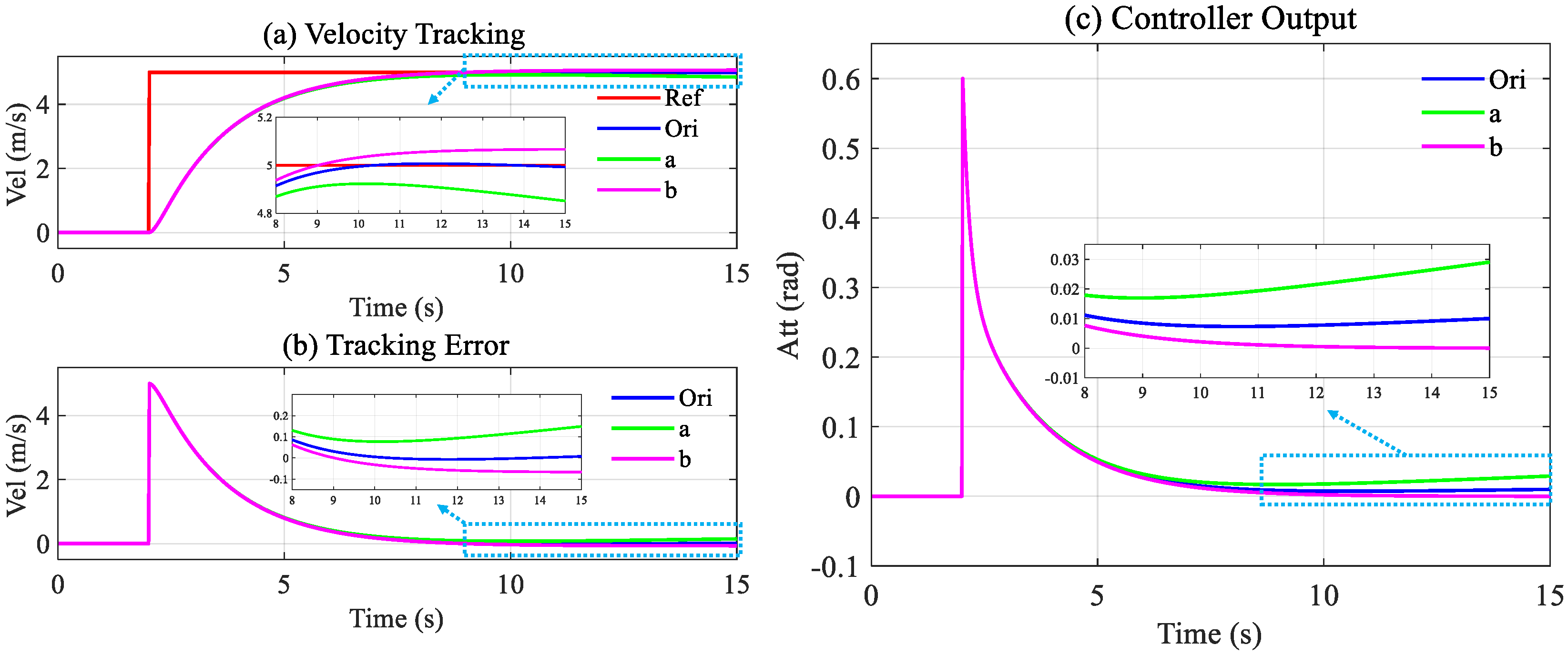
Based on the original system, m was reduced and increased, respectively, and marked as ‘a’ and ‘b’ according to the change order of −2 kg and +2 kg. The tracking results for Method A and the controller’s output are shown in Figure 10.

After the weight parameter changes, the simulation results showed that Method A can always track the target. However, the tracking accuracy has apparent differences. From Figure 10b, it can be seen that the tracking error is close to 0.2 m/s at 15 s in case ‘a’ and close to 0.1 m/s in case ‘b’.

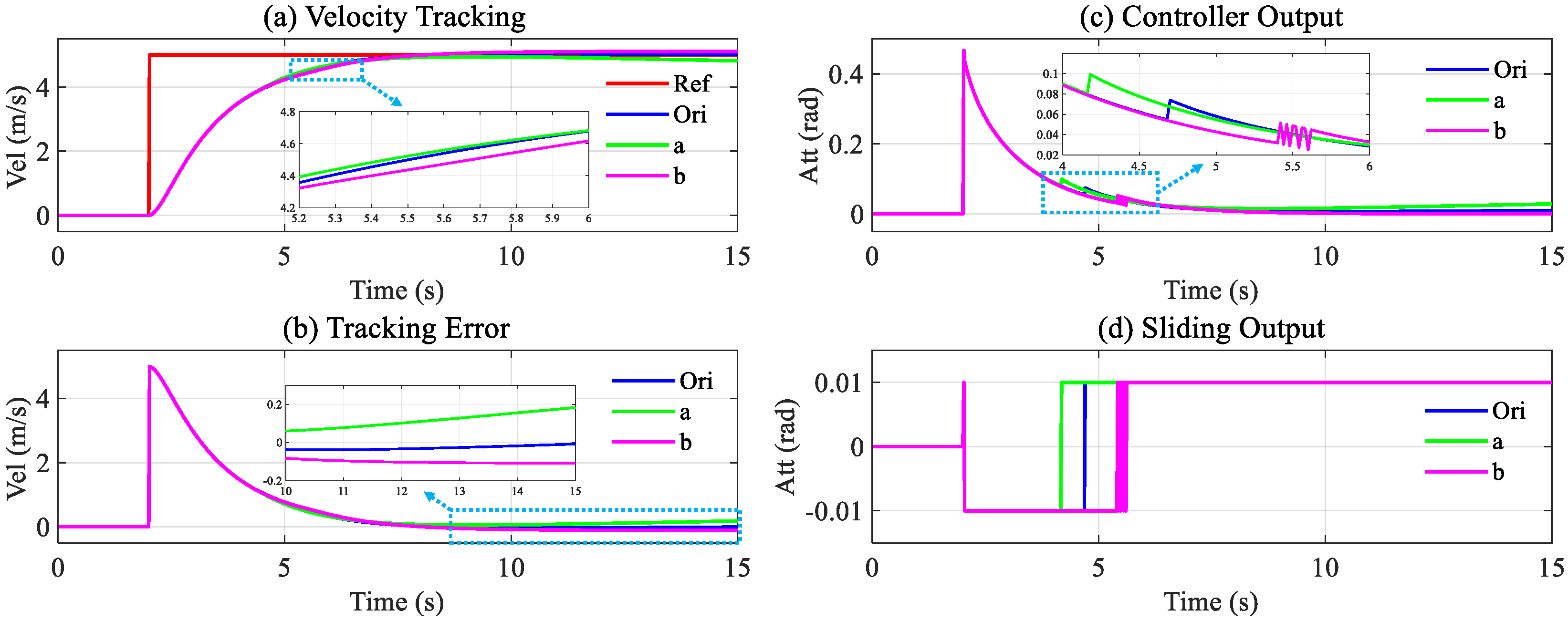
The simulation results of Method B for the changes in quality are shown in Figure 11.

The simulation results for Method B are similar to that for Method A. Method B can maintain the tracking with an increase in the tracking error, and the sliding output has different performance values between 4 s and 6 s, as seen in Figure 11c,d and is also reflected in Figure 11a.

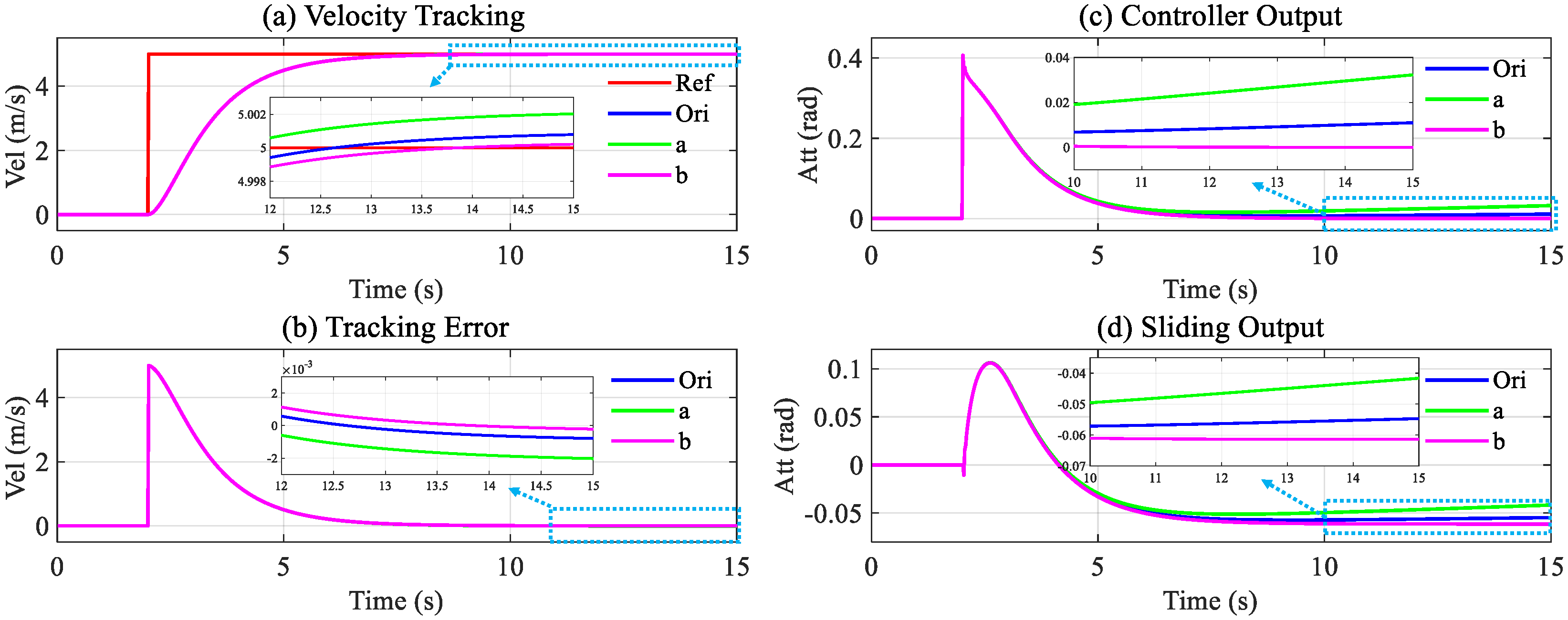
Different from Methods A and B, the parameter changes have little impact on Method C, as shown in Figure 12. Compared with the two former kinds of tracking error, the steady-state tracking error differs in the order of magnitude. It can be seen in Figure 12b that case ‘a’ with the most significant tracking error at 15 s is only 0.002 m/s.

The velocity tracking error of the three methods in all three cases are summarized in

Table 3. Tracking error of the three methods in all three cases.

	Case Ori		Case a		Case b
Method	Mean	Variance	Mean	Variance	Mean	Variance
A	0.5559	1.2232	+0.0494	−0.0480	−0.0257	+0.0268
B	0.5209	1.2556	+0.0596	−0.0626	−0.0231	+0.0313
C	0.4923	1.2146	−0.0007	+0.0006	+0.0004	−0.0003

. It should be noted that the three schemes are mainly used to verify the robustness of unknown parameters, and indicators such as the rise time are not considered. Therefore, comparing the three algorithms with their respective initial situations is valuable. Hence, in the columns for cases ‘a’ and ‘b’, the statistical data represent the changes compared to the original case.

It can be seen from Table 3 that the proposed method has clear advantages in the case of parameter changes. Compared with the original case, the mean and variance of the tracking error changes are the tiniest. It can be demonstrated that the proposed scheme shows a satisfactory robustness against the parameter uncertainty.

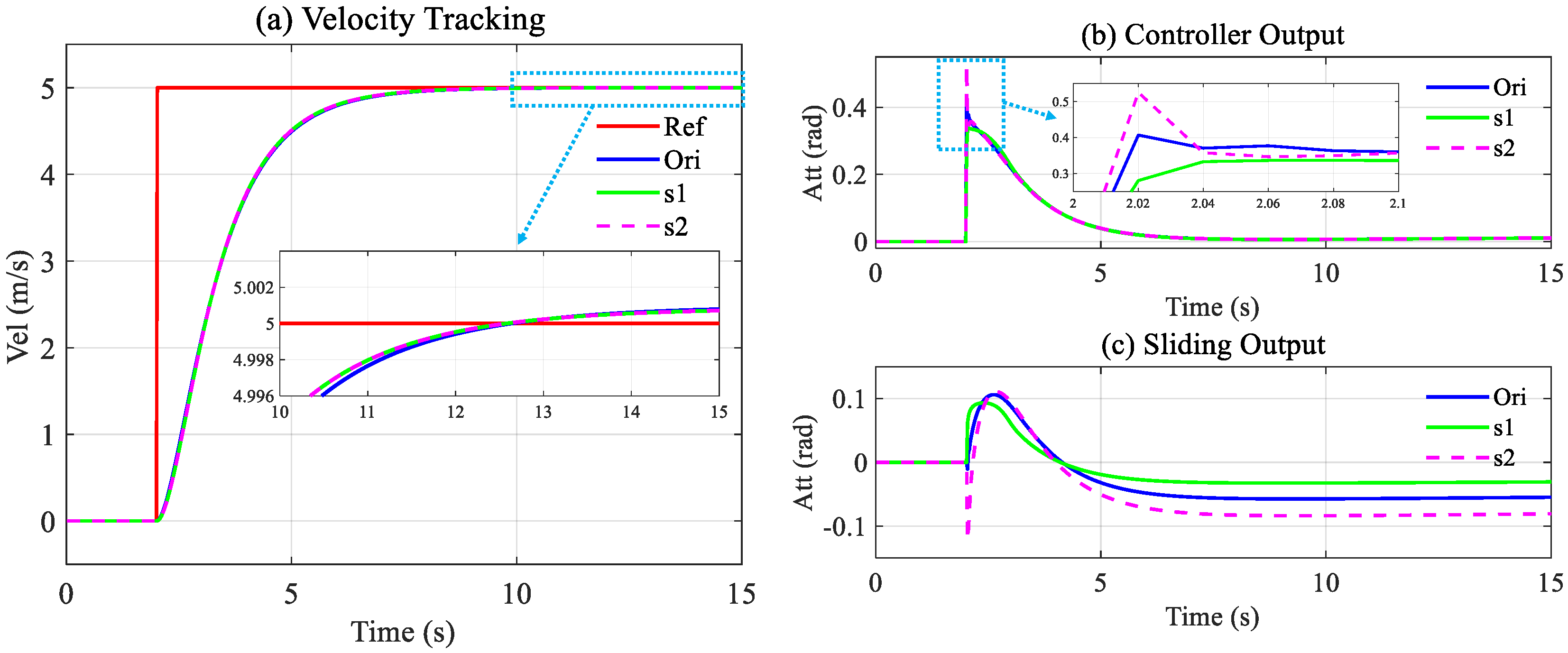
4.3.2. Modeling Robustness Verification

After the verification in Section 4.3.2, it can be said that the proposed method based on the original model has a stable performance under the change in m. However, considering that the method is implemented based on a data-driven model, there is still a need to explore whether the deviation in the model-fitting process will affect the final controller.

Modifications to the fitted data mimic the biases in the model’s data collection process. Thus, based on the deviation model, we designed the controller according to the steps described in Section 4.2 and applied it to the initial model. We simulated two cases denoted as ‘s1’ and ‘s2’.

In s1, $K_{Att}$ = 0.8, $T_{Att}$ = 0.3, and m = 5 kg.

In s2, $K_{Att}$ = 1.0, $T_{Att}$ = 0.2, and m = 4 kg.

The selection of the parameters was based on the random adjustment of the original. The results of the two cases acting on the initial model are shown in Figure 13.

From Figure 13a, it can be seen that the velocity tracking effect is similar to the original situation in the case of ‘s1’ and ‘s2’. However, Figure 13b,c show that there are certain differences in the output, calculated by the controller. The change in the sliding output in Figure 13c sufficiently reflects the strong robustness in the face of unknown parameters. From the simulation results, the proposed method can be said to be robust against deviations in the model acquisition process.

4.4. Experiment Validation

The proposed method shows a strong robustness in the simulation; however, its effect on the actual environment needs further verification. Therefore, we arranged target-tracking, fixed-point hovering, and robust verification experiments. In the experiments, the PID algorithm was selected for the comparison.

4.4.1. Target Tracking

In the target-tracking experiment, the self-defined velocity target consisted of three types: sine wave, step about 6.25 m/s, and hover. The experimental results are shown in Figure 14 and Figure 15.

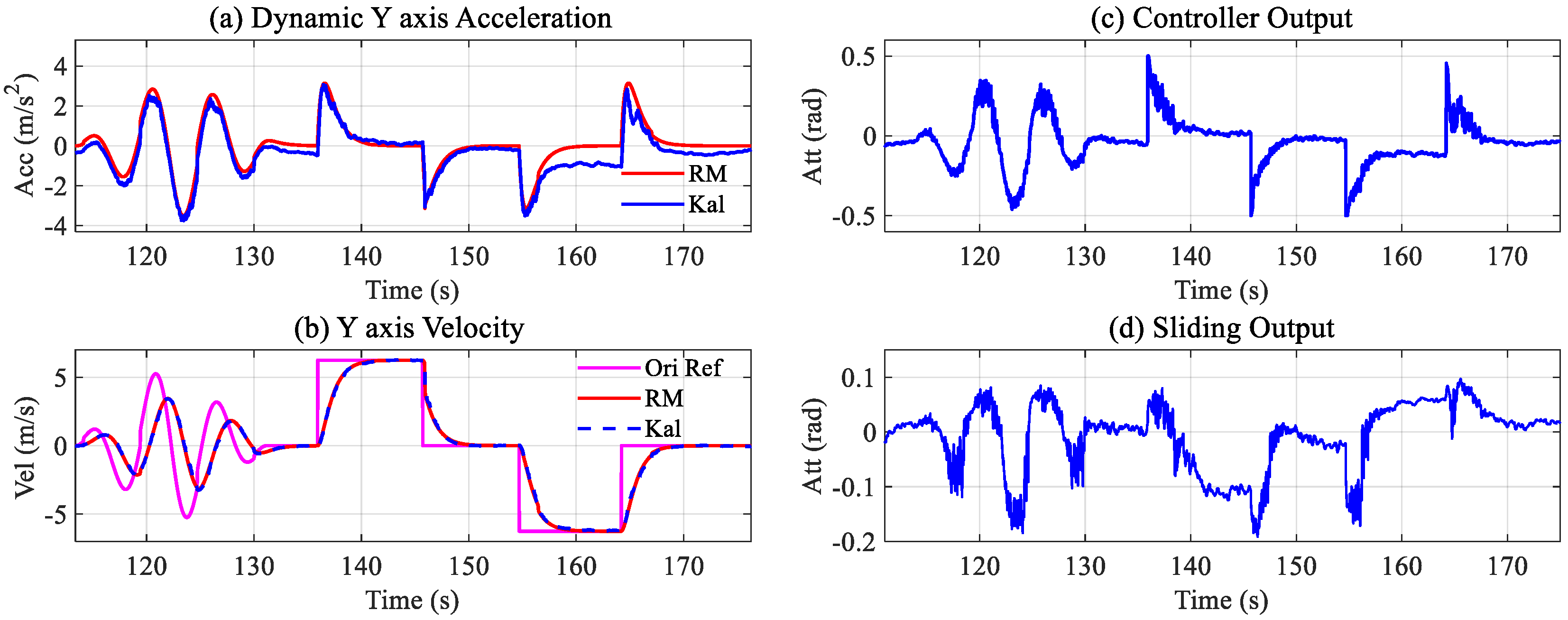
Figure 15 shows the tracking results of the self-defined target signals. Figure 15b depicts the reference and tracking of the velocity. The reference model calculates the reference signal corresponding to the original target; it can be seen that the estimated velocity can follow the reference accurately. Figure 15a shows the tracking of the dynamic acceleration. The UAV keeps hovering at 160 s; however, the estimated dynamic acceleration does not converge to 0 m/s${}^2$. The Kalman estimate result in Figure 14 shows that the roll is 0.1 rad at the same time. After the analysis, it was found that the deviation in the center of gravity is a major factor that brings an attitude bias in the hovering. In the state estimation process, the dynamic acceleration is related to the attitude; thus, the estimated acceleration when the UAV hovers cannot reflect the actual situation.

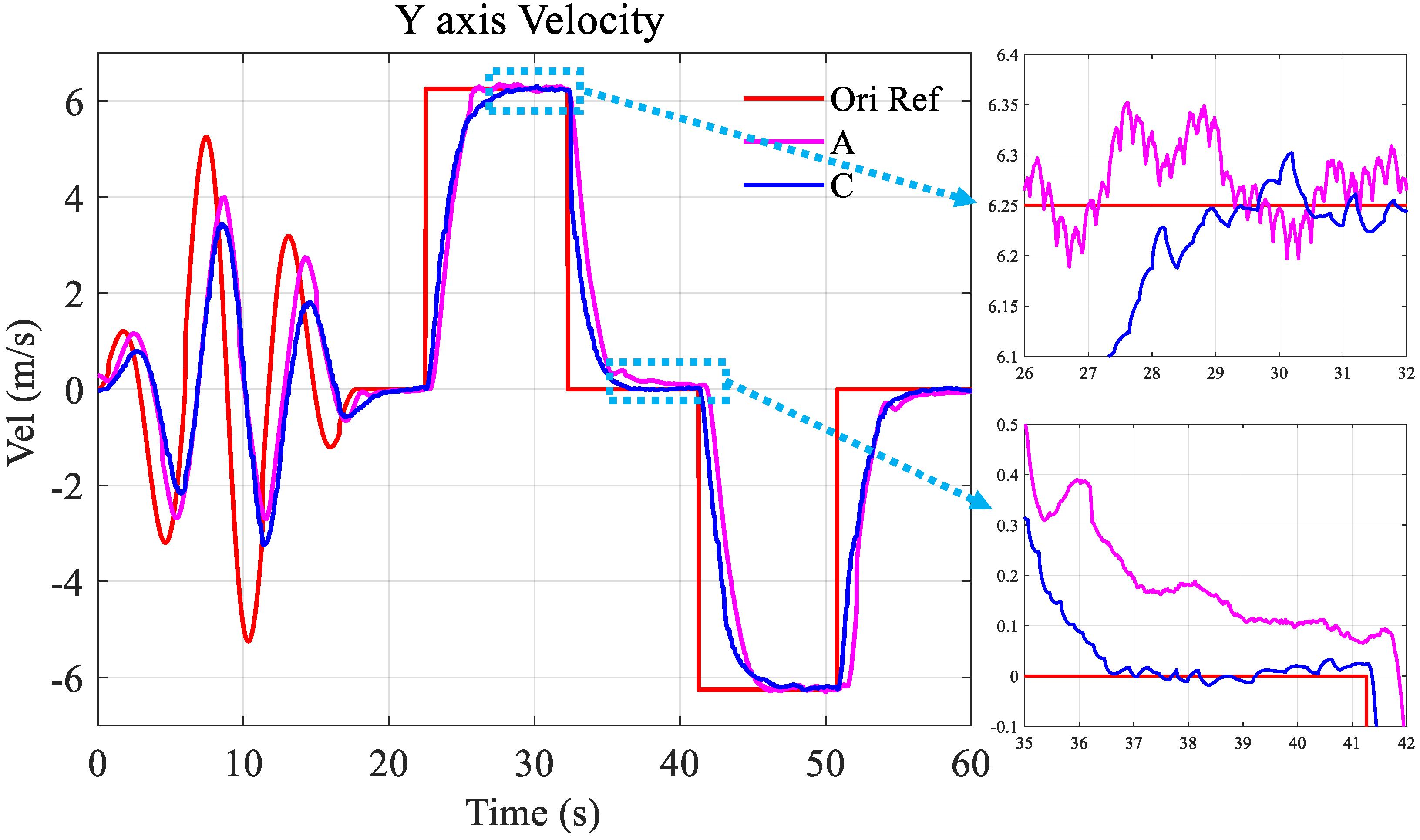
Under the gravity center deviation and the sensor measurement noise, the velocity controller designed with Method A was also implemented. The results of the two experiments are shown in Figure 16.

In Figure 16, it can be seen that there are no significant differences between the two methods in terms of the dynamic tracking and hovering. However, for the step response at 27 s and 36 s, the stability of Method A could be better. Due to the deviation in the gravity center, Method A showed different results for the target value in the opposite direction, while Method C remained consistent.

4.4.2. Fixed-Point Hovering

In the fixed-point hovering experiment, the stability of the proposed method was verified by the autonomous velocity target calculation with the position controller. The UAV hovered outdoors with a gust of 3–5 m/s for more than 3 min to avoid randomness in the experiment. Methods A and C were applied in the same experimental environment and with the same position controller. 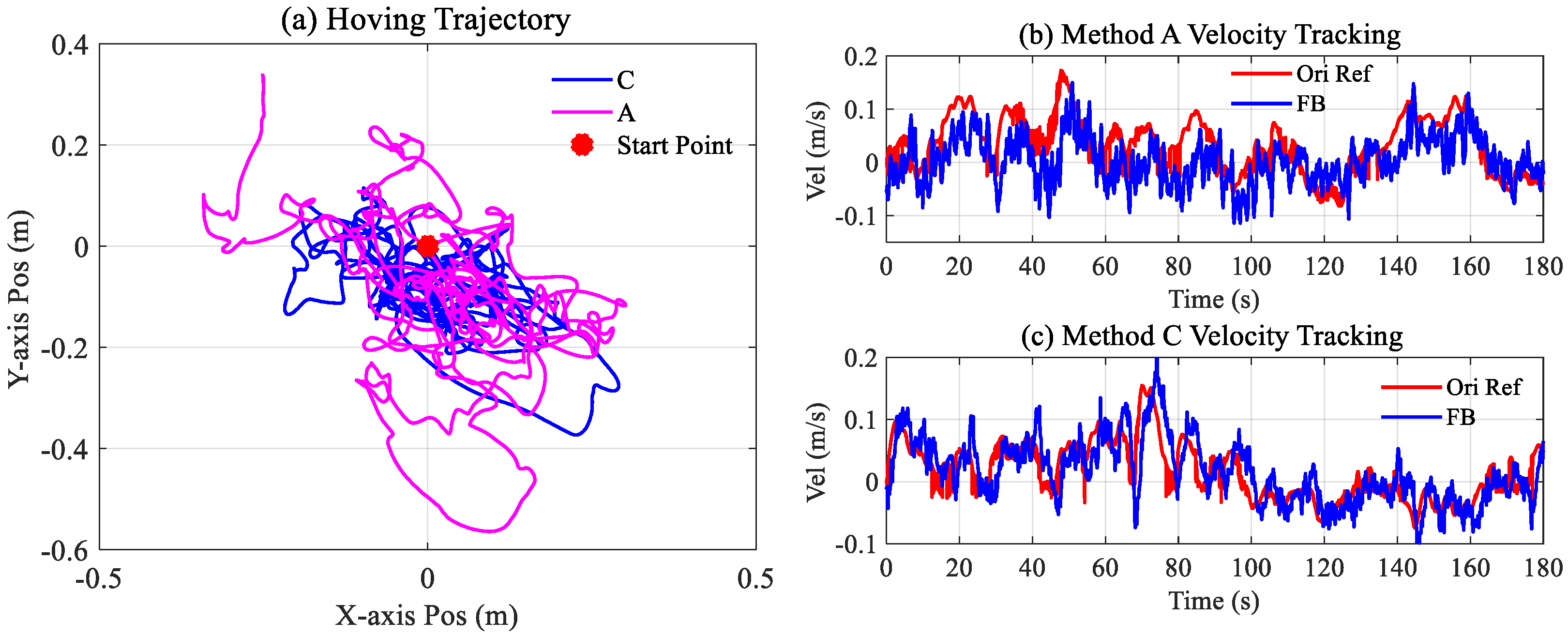The experimental results are shown in Figure 17 and Figure 18.

Figure 17a records the dynamic trajectories of the two methods during the hovering. In contrast, the blue curve shows more compactness. Figure 17b,c show the two methods’ velocity reference and feedback. In Figure 17b, it can be seen that there are several situations where the velocity target could not be tracked well, such as 40–50 s, 60–70 s, and 80–90 s. In contrast, this phenomenon was not found in Figure 17c.

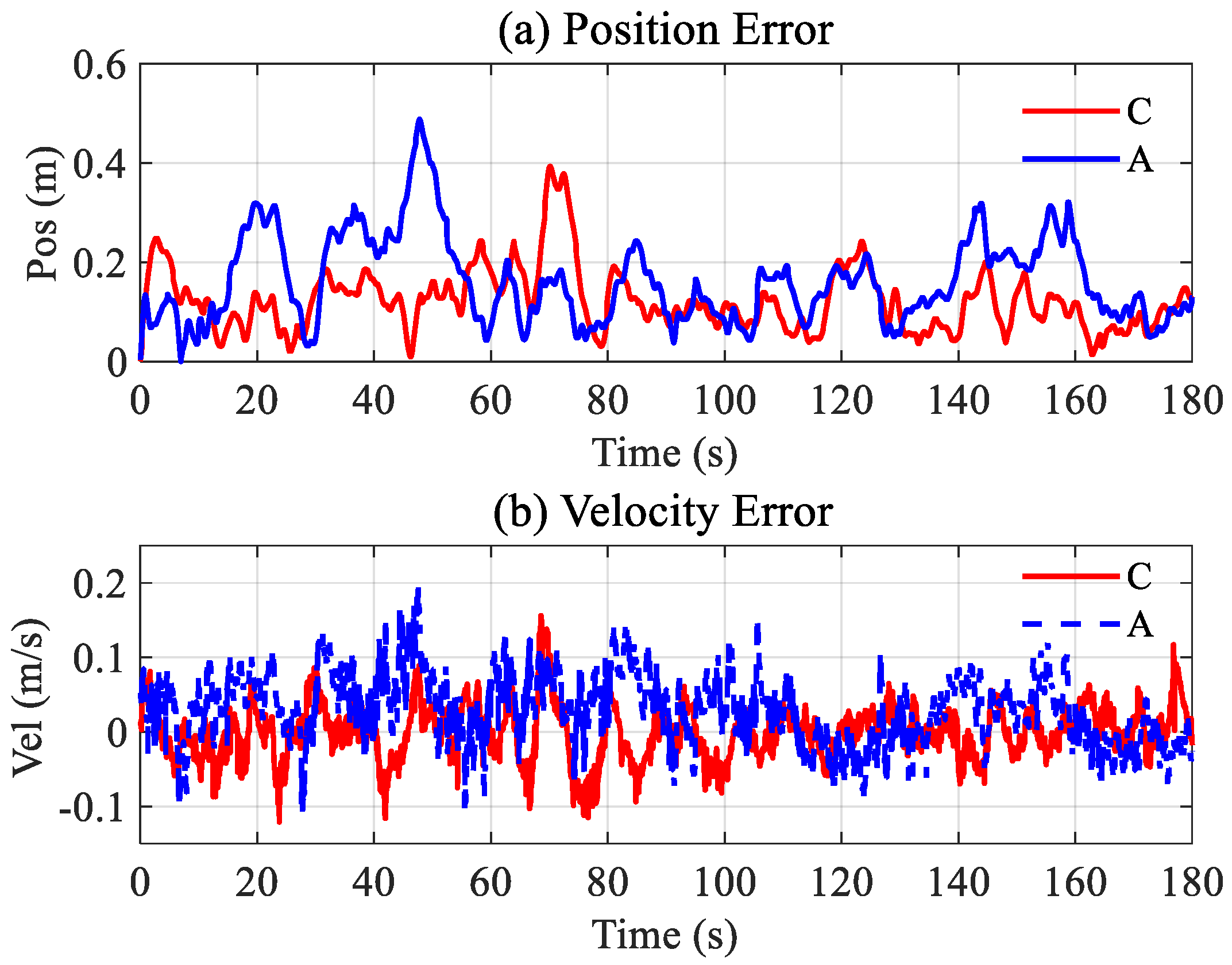
The tracking errors of the position and velocity during the hovering are shown in Figure 18a,b, respectively. It can be seen that the position error of Method A is more noticeable compared to Method C, with an average of approximately 0.2 m; further, the velocity tracking error has a more evident amplitude fluctuation over 100–180 s.

4.4.3. Robust Verification

In industrial applications, UAVs are expected to carry different payloads to accomplish various tasks. Herein, this process was simulated by adding weights. We added a weight of 4.86 kg to the bottom plate of the six-rotor UAV, as shown in Figure 19. After adding the load, the take-off weight changed from 5.96 kg to 10.82 kg.

The self-defined target in the target-tracking experiment was used, and the results are shown below.

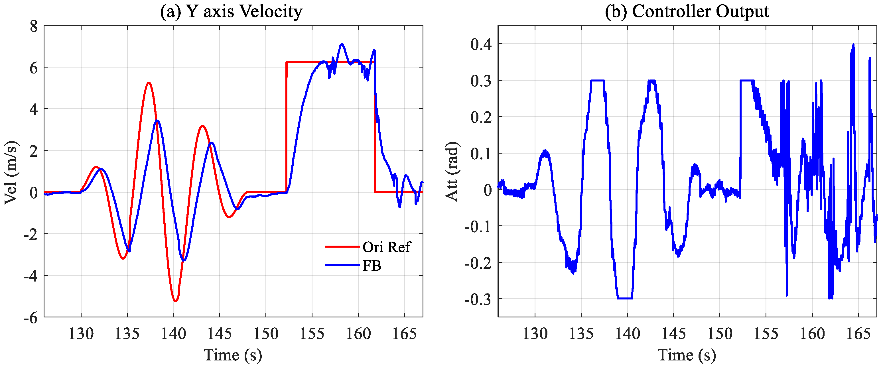
Figure 20 shows the velocity tracking of Method A after loading. There is a large gap between the actual flight and the simulation results. The dynamic model has changed after increasing the weight to 10.82 kg, and the change is yet to be fully reflected in the simulation.

After increasing the load, the dynamic tracking of the continuous sine signal can still be realized; however, there are noticeable differences in the step situation. From the controller output in Figure 20b, we can find that the controller outputs smoothly when tracking the target. However, once the target signal is followed, the controller’s output becomes extremely unstable.

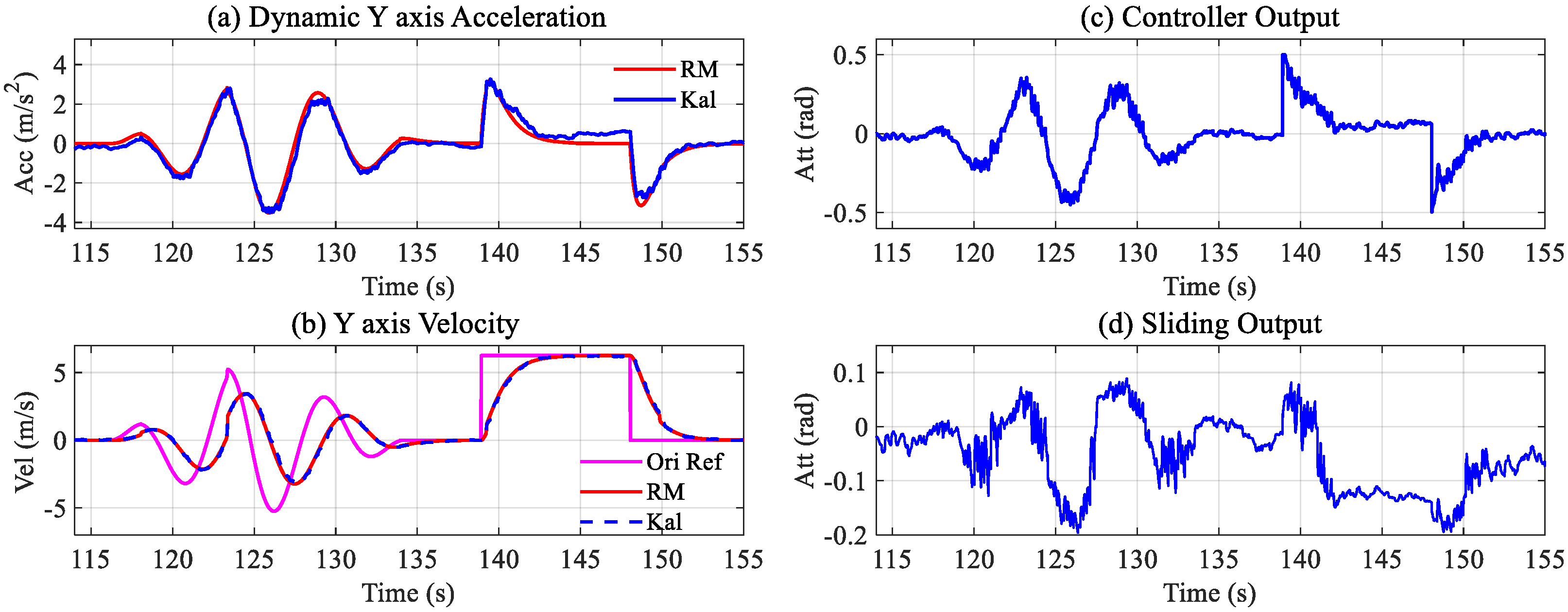
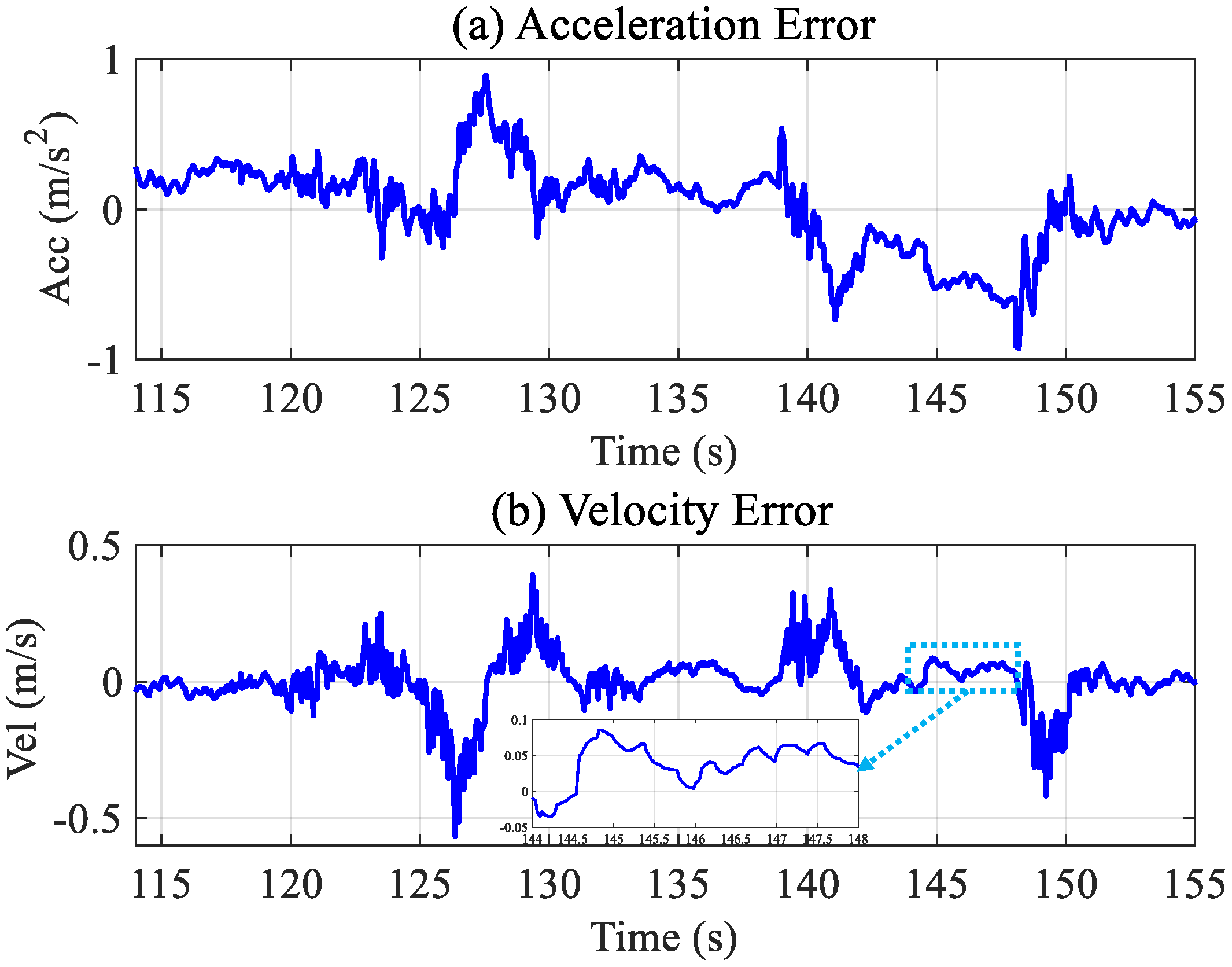
The tracking of Method C after loading is shown in Figure 21. Compared with the no-load situation, the noticeable change in the acceleration tracking effect has deteriorated. Comparing the tracking performance in the same period, the statistics of Method A and C with and without the payload are shown in

Table 4. Tracking error of the two methods with and without payload.

	Without Payload		With Payload
Method	Mean	Variance	Mean	Variance
A	0.1079	3.0885	+0.0122	+0.5324
C	0.0759	4.1935	+0.0019	+0.1696

.

Table 4 shows that compared with the case without the payload, the mean of the tracking error of Method A increased 11.3%, and the variance increased 17.2% after the payload was added. However, the mean and variance of the proposed Method C target only changed 2.5% and 4%, and the velocity can maintain a stable tracking performance.

Figure 22 shows the tracking error between the acceleration and velocity. When the velocity catches up with the target, it can be kept within ±0.1 m/s of it, as shown by 144–148 s in Figure 22b. Relative to the target velocity of 6.25 m/s, the steady-state error can be negligible.

5. Conclusions

In this work, we proposed and implemented a reference model based on an integral SMC method to deal with the problem of parameter uncertainty, especially concerning significant load changes. The method consists of a steady-state Kalman filter, a reference model, and an integral sliding mode controller. The design process was described in detail by taking the velocity control as an example. Various simulations, such as the controller robustness verification under the model variation and the modeling robustness under the controller parameter variation, were conducted. The robustness against the parameter uncertainty was verified via a comparison with an LQR-based integral SMC in the simulation. Finally, we applied our method to a six-rotor UAV and executed three flight experiments, including target tracking, fixed-point hovering, and robust verification. In the robust verification, we used an astonishing 81.5% load variation, and under such conditions, our method still achieved satisfactory results.

The proposed scheme is based on the fitted model that only needs to collect the data during flying, and the controller is robust to the fitted model. However, the verification process was conducted in a natural environment, and significant external disturbances were not considered. As far as we know, the controller stability will be reduced with an increase in the external disturbance. In addition, our work only verifies the velocity tracking in the single-axis direction, and the velocity and position in the vertical direction are not considered. Therefore, the full-axis velocity control for disturbed environments deserves to be further studied, and the position information will also be considered in our future research.