Article

A Novel Adversarial Detection Method for UAV Vision Systems via Attribution Maps

School of Information and Software Enginerring, University of Electronic Science and Technology of China, Chengdu 610054, China
*
Author to whom correspondence should be addressed.
Drones 2023, 7(12), 697; https://doi.org/10.3390/drones7120697
Submission received: 19 September 2023 / Revised: 29 November 2023 / Accepted: 6 December 2023 / Published: 7 December 2023
(This article belongs to the Special Issue UAV-Assisted Internet of Things)

Abstract

:
With the rapid advancement of unmanned aerial vehicles (UAVs) and the Internet of Things (IoTs), UAV-assisted IoTs has become integral in areas such as wildlife monitoring, disaster surveillance, and search and rescue operations. However, recent studies have shown that these systems are vulnerable to adversarial example attacks during data collection and transmission. These attacks subtly alter input data to trick UAV-based deep learning vision systems, significantly compromising the reliability and security of IoTs systems. Consequently, various methods have been developed to identify adversarial examples within model inputs, but they often lack accuracy against complex attacks like C&W and others. Drawing inspiration from model visualization technology, we observed that adversarial perturbations markedly alter the attribution maps of clean examples. This paper introduces a new, effective detection method for UAV vision systems that uses attribution maps created by model visualization techniques. The method differentiates between genuine and adversarial examples by extracting their unique attribution maps and then training a classifier on these maps. Validation experiments on the ImageNet dataset showed that our method achieves an average detection accuracy of 99.58%, surpassing the state-of-the-art methods.

1. Introduction

The rapid advancement in the fields of unmanned aerial vehicles (UAVs) and synthetic aperture radar (SAR) has led to significant breakthroughs in remote sensing capabilities [1,2]. The integration of SAR technology with UAVs [1,2] has unlocked the potential for acquiring high-definition imagery from above, providing a versatile tool for detailed surveillance and analysis across vast and varied landscapes. Building upon this development, these high-resolution SAR images captured by UAVs are revolutionizing the Internet of Things (IoT) landscape by enriching the spectrum of data available for automated processing and interpretation. In the realm of IoTs, UAVs equipped with vision systems have become pivotal in tasks requiring extensive area coverage with precision, such as monitoring wildlife migration patterns in their natural habitats or providing real-time data on environmental conditions for ecological studies.
Meanwhile, deep neural networks (DNNs) have proven to be particularly effective in processing the complex data obtained from SAR images [3,4]. Their advanced representation capabilities facilitate accurate analysis and have been instrumental in the development of SAR automatic target recognition (SAR-ATR) models [5,6,7,8]. By leveraging the computational prowess of DNNs, these models have rapidly gained popularity due to their efficiency and reliability in identifying and classifying targets in diverse environments.
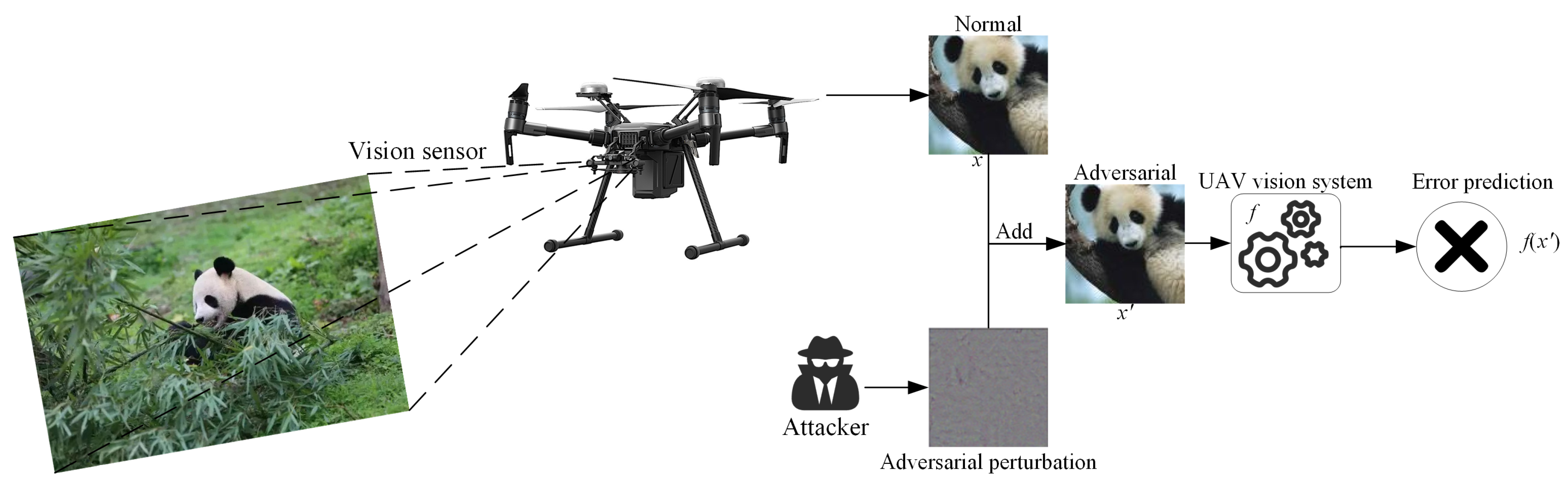
Although the integration of DNNs into UAV vision systems has markedly improved their capability to deal with complex data, it has concurrently opened up a vector for a new type of threat—adversarial attacks [9]. These attacks are executed through the generation of adversarial examples, which are seemingly normal images that have been meticulously modified with imperceptible perturbations. These alterations are calculated and crafted to exploit the inherent vulnerabilities of DNNs, causing them to misinterpret the image and make incorrect decisions [10]. The process of its attack implementation is shown in Figure 1. Such adversarial attacks on UAV vision systems can lead to unpredictable behavior and severely impact the security of data acquisition and transmission in UAV-assisted IoTs [11]. In scenarios where UAVs are employed for critical missions, such as search and rescue operations, security surveillance, or precision agriculture, a false classification could lead to dire outcomes. For instance, an adversarial image could cause a UAV to overlook a lost hiker it was tasked to locate or misidentify a benign object as a security threat, triggering unwarranted responses. Moreover, the challenge is exacerbated by the fact that these perturbations are designed to be imperceptible to human analysts, which means that the reliability of UAV systems could be compromised without immediate detection. This underlines the urgency for the research and development of defense strategies that can detect and neutralize adversarial examples before they impact UAVs.
In order to address this emerging threat, researchers propose two defense strategies: active and passive defense strategies. Active defense methods increase the robustness of models against adversarial attacks through techniques like adversarial training [12,13] and network distillation [14], which are applied during training. In contrast, passive defense involves detecting and filtering adversarial inputs during model deployment. Our research focuses on passive defense, aiming to identify features that differentiate adversarial from clean samples, thereby enabling the detection of adversarial examples and safeguarding the model from potential attacks.
As a reflection of the ongoing efforts in the deep learning community, there is intensive research on adversarial detection. Numerous passive defense techniques have been developed to tackle adversarial attacks. Hendrycks and Gimpel [15] proposed three methods: Reconstruction, PCA, and Softmax, which, while effective against FGSM [9] and BIM [16] attacks, have limitations in detecting more sophisticated threats. Metzen et al. [17] developed an adversarial detection network (ADN), which enhances binary detection in pretrained networks and shows promise against FGSM, DeepFool [18], and BIM attacks but not against the more challenging C&W [19] attacks. Gong et al. [20] made further attempts to improve an ADN, yet it remained inadequate for C&W attack detection. Xu et al. [21] suggested that adversarial example generation is linked to excessive input dimensions and introduced feature squeezing to identify adversarial instances by contrasting the outputs of squeezed and original samples. This approach shows potential in detecting C&W attacks, but its precision still requires enhancement.
In summary, while the aforementioned methods show efficiency in detecting adversarial attacks, such as FGSM and BIM, they fall short when faced with more potent threats like the C&W attack.
Building on this premise, researchers have demonstrated that the adversarial perturbations from C&W attacks tend to be subtler than those from other methods like FGSM when executed under comparable conditions [22]. As a result, adversarial examples crafted via C&W attacks are notably more challenging to detect. In this paper, we classify such finely perturbed instances as strong adversarial examples typified by the C&W attack. In contrast, examples with more pronounced perturbations, like those from FGSM attacks, are deemed weak adversarial examples.
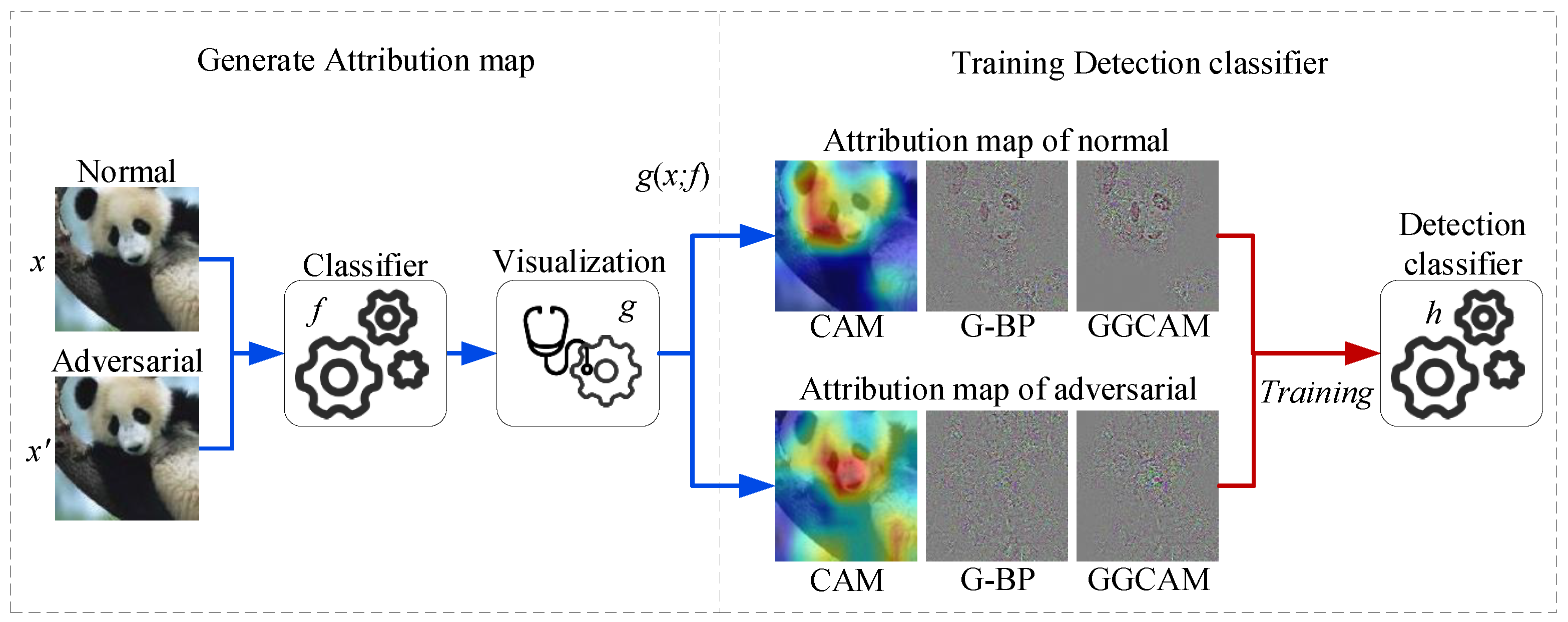
Additionally, recent studies have revealed that the convolutional layers in convolutional neural networks (CNNs) inherently function as object detectors, even without explicit object location supervision. Consequently, visualizing the model by extracting the features detected by each CNN layer is possible. In this paper, we have expanded upon earlier versions [23]. We have added a significant amount of more detailed charts, conducted adversarial detection experiments based on different attribute maps, and further compared our method with several state-of-the-art approaches. We propose an adversarial detection method for UAV vision systems based on different attribution maps. The proposed methods consist of two steps. Firstly, we generate attribution maps for both clear and adversarial samples using three different types of attribution maps, including class activation mapping (CAM) [24], guided backpropagation (G-BP) [25], and guided Grad-CAM (GGCAM) [26]. We then tried to train a binary classifier by using the generated attribution maps to detect adversarial samples. Through experiment analysis, there are distinguishing features between the attribution maps of clear and adversarial samples. In particular, the G-BP and GGCAM of clear samples have discrimination contour features, but after adversarial perturbations are added, the contour features are destroyed, showing that the attribution maps generated by model visualization techniques can effectively distinguish adversarial samples from clear samples. We conducted experiments on ImageNet, and the results show that when using three different attribution maps, this method can detect not only weak adversarial samples, such as FGSM and BIM, but also strong adversarial samples, like C&W. Among them, the detection success rate achieved using G-BP reached up to 99.58%, surpassing the state-of-the-art methods.
The main contributions of this paper are as follows:
(1) This paper presents novel model visualization techniques that are introduced for the first time to detect adversarial examples. Model visualization approaches are employed to analyze sample features, and we find the attribution maps of adversarial and clear samples differ considerably. Specifically, the contour features of G-BP and GGCAM are destroyed when the adversarial perturbations are added.
(2) We propose a novel adversarial detection method for UAV vision systems via attribution maps. When using different attribute maps, the success rate of adversarial sample detection can reach more than 90%. Among them, the detection success rate based on the G-BP map can reach 99.58%, which is 1.68% higher than the state-of-the-art method.

2. Related Works

2.1. Adversarial Attacks

Szegedy et al. [9] first presented the concept of adversarial perturbations. By leveraging gradient information, they skillfully introduced subtle perturbations to original images. These minor modifications transformed clean samples into adversarial examples. While often imperceptible to the human eye, these examples can mislead classifiers into making incorrect predictions. Based on their operational domain, current research primarily categorizes adversarial examples into digital and physical attacks.
Let x R d denote a clean image sample, with x a d v representing its corresponding adversarial example. The adversarial perturbations can be represented as an optimization problem:
arg max x adv J ( x adv , y ) s . t . x adv x l p ϵ
where J ( . ) denotes the loss function, which measures the error magnitude of the adversarial example x a d v in relation to y, the ground-truth label of x. | | x a d v x | | L p signifies the l p -norm distance between x a d v and x, typically utilizing norms, p = { 0 , 2 , } . ϵ is a threshold that restricts the magnitude of the perturbation, implying that the difference between the adversarial and the original samples should remain within a narrow and explicitly defined boundary.
Adversarial attacks involve perturbing input images at the pixel level to mislead DNN predictions. Depending on the knowledge of attackers about the target model, digital attacks can be categorized into white-box attacks and black-box attacks. In white-box scenarios, attackers have full access to all information about the target model, enabling them to effectively exploit model gradients to craft precise perturbations and misguide model predictions [9,19,27,28,29]. Conversely, under black-box assumptions, attackers have no knowledge of the target model and can only query the model to obtain its outputs. Such attackers often capitalize on the transferability of adversarial examples between different models [30,31,32,33] or reveal the inner structure of the model through repeated queries [34,35,36,37]. Sometimes, attackers even combine both approaches for more potent attacks [38].

2.2. Adversarial Example-Detection Technology

Adversarial example-detection technology can be roughly divided into two stages. In the early stage, researchers mainly explore the difference between adversarial and clear samples. Hendrycks et al. [15] proposed principal components analysis (PCA) and found that the variance in the principal components of adversarial examples is usually larger than that of clean samples. At the same time, they also found that adversarial samples will emphasize the main components with a lower ranking in PCA abnormality. Therefore, they combined these two findings to design the adversarial sample detection method based on PCA, which can detect FGSM and BIM adversarial samples. However, this method is only effective if the attacker is unaware of the defense strategy. Hendrycks et al. also found that the Softmax outputs of adversarial and clear samples are different in several types of attacks, so the adversarial samples can be detected by detecting the Softmax distribution. However, Softmax distribution is not stable, which generally leads to low confidence in the prediction, and this method is only applicable to specific attacks. Xu et al. [21] found that higher-dimensional input features are more vulnerable to adversarial attacks. Therefore, they proposed the feature squeeze method. The main idea of this method is to squeeze the dimension of input features by removing unnecessary features. If the L1 norm difference between the prediction of squeezed and unsqueezed inputs is larger than some threshold, T, the input is marked as an adversarial sample. Feature squeeze has been shown to detect FGSM, BIM, DeepFool, and C&W attacks. Based on the assumption that adversarial samples are not non-adversarial data manifolds, Feinman et al. [39] proposed two adversarial detection methods: kernel density estimates (KDEs) and Bayesian uncertainty estimates (BUEs). The purpose of KDEs is to determine whether data are far from the class manifold, and BUEs can detect the data near the regions with low confidence when the KDEs are invalid.
Currently, adversarial detection typically involves decomposing input samples and analyzing the extracted features to identify adversarial examples. Metzen et al. [17] introduced an adversary detection network (ADN) to safeguard deep neural networks (DNNs). The ADN employs a binary detector network appended to a pretrained neural network. This detector is trained to differentiate between adversarial and genuine samples. Across 10 subsets of CIFAR10 and ImageNet, the authors successfully trained a highly accurate adversarial detection network using ADN. In order to enhance the detector’s resilience against new attacks, they incorporated the generation of adversarial examples into the ADN training process. This approach effectively detects FGSM, DeepFool, and BIM attacks. Gong et al. [20] further refined the ADN method by training a binary classifier that operates independently of the main classifier. Unlike previous methods that tailor adversarial samples to the detector, this technique uses adversarial samples generated against the pretrained classifier to augment the original training dataset, which, in turn, trains the binary classifier. Nevertheless, Carlini et al. [40] noted that such methods yield a high false-positive rate when confronted with more potent attacks like the C&W. While these strategies are adept at detecting weaker adversarial examples, such as those from FGSM and BIM, their detection accuracy decreases against stronger attacks, exemplified by the C&W.

2.3. Model Visualization Methods

Model visualization techniques play a pivotal role in enhancing the transparency and interpretability of deep learning models. Marco et al. [41] proposed a method of local interpretable model agnostic explanations (LIMEs). LIMEs provide a local approximation of the behavior of models, which can be incredibly insightful when trying to understand individual predictions. However, its locality and linear approach might not capture the global complexity of the model. On the other hand, CAM, proposed by Zhou et al. [24], offers a straightforward mechanism for highlighting influential regions in an image for a given prediction. Yet, as mentioned, its reliance on model modification and retraining can be resource-intensive and may not be feasible for all applications. While post-interpretability methods like LIME and CAM have laid the groundwork, there is a continuous effort to refine these approaches to minimize their limitations and expand their applicability. In order to address these concerns, Grad-CAM [26] emerged as a versatile and powerful tool that extends the capabilities of CAM without the need for structural modifications or retraining. By utilizing the gradients flowing into the final convolutional layer, Grad-CAM provides a fine-grained visualization of the areas impacting the model’s decision-making process. Building on the strengths of Grad-CAM, recent advancements have introduced more sophisticated techniques that further refine the interpretability of convolutional neural networks. One such development is Grad-CAM++ [42], an extension that captures the importance of each feature map for a particular class, allowing for even more detailed visual explanations.

3. Methodology

In recent years, researchers have studied the interpretability of DNNs from two aspects: models [43,44,45] and samples [40,46,47]. This paper approaches the issue of adversarial example detection from the sampling perspective, utilizing model visualization techniques to produce attribution maps for both clean and adversarial samples, thereby investigating their distinguishing features. It is acknowledged that the smaller the perturbations in adversarial examples, the more challenging they are to detect. Consequently, this study opts for untargeted attacks to generate adversarial samples, aiming to minimize the perturbations introduced.
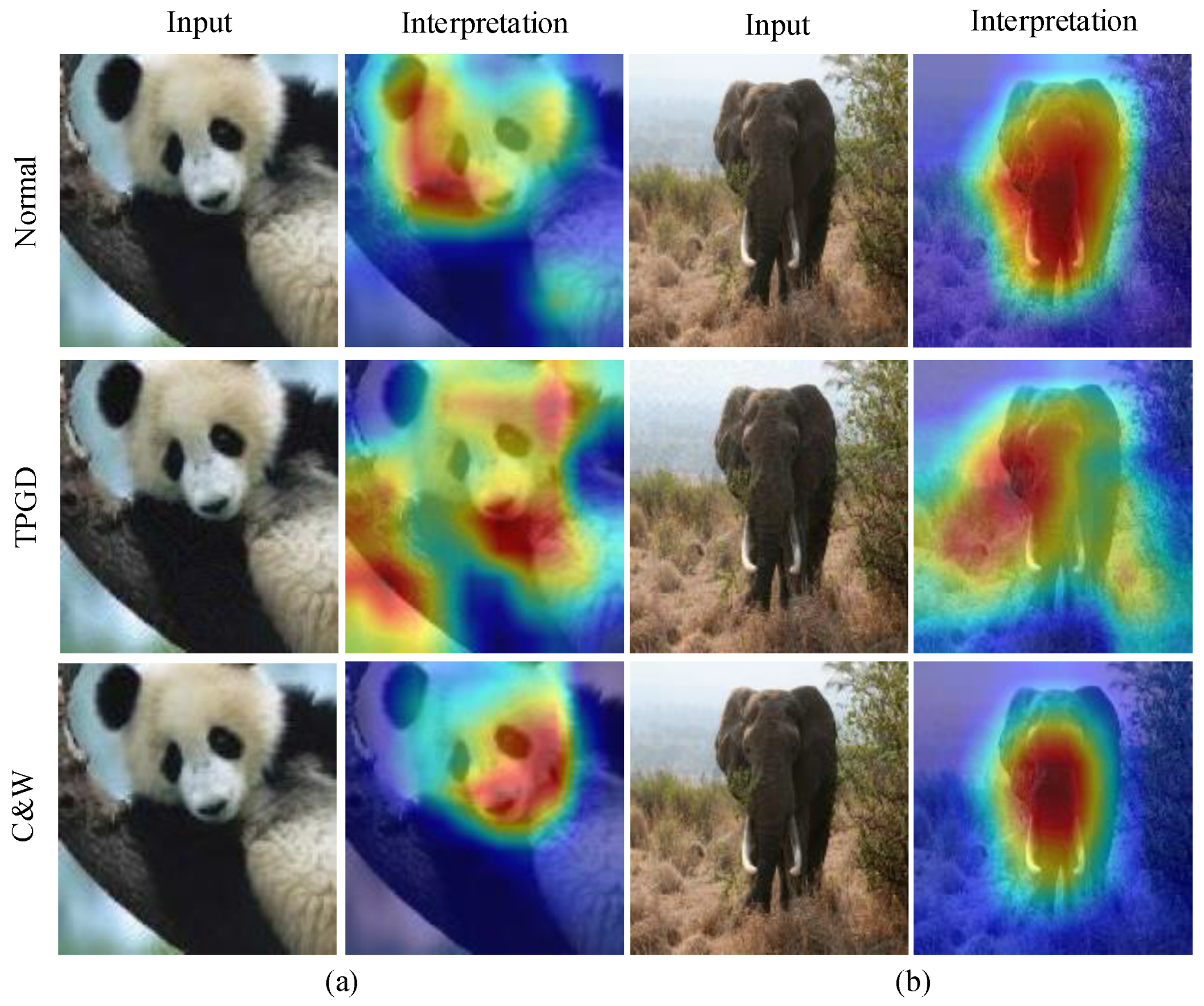
Inspired by the study of model interpretability [48], we find a large gap between the CAM of normal and adversarial samples. So, for example, we select two samples and transform them into adversarial samples by using the C&W and TPGD [49] methods. Then, we compare their CAMs, as shown in Figure 2. Normal represents the clear sample and its corresponding attribution map. The highlighted part contains the most abundant input information, revealing the causal relationship between model output (classification) and input. The row of TPGD is the adversarial samples and their corresponding attribution maps generated by the TPGD method. The highlighted part of the attribution map of the adversarial sample shows a great change, which has a high degree of differentiation compared with the attribution map of normal samples. Meanwhile, it also reveals the causal relationship between model misclassification and perturbation input. Similarly, the third row presents adversarial samples and their attribution maps created by C&W. When compared to TPGD, the differences in attribution maps with C&W are much less pronounced, confirming the strength of C&W as a white-box attack [22].
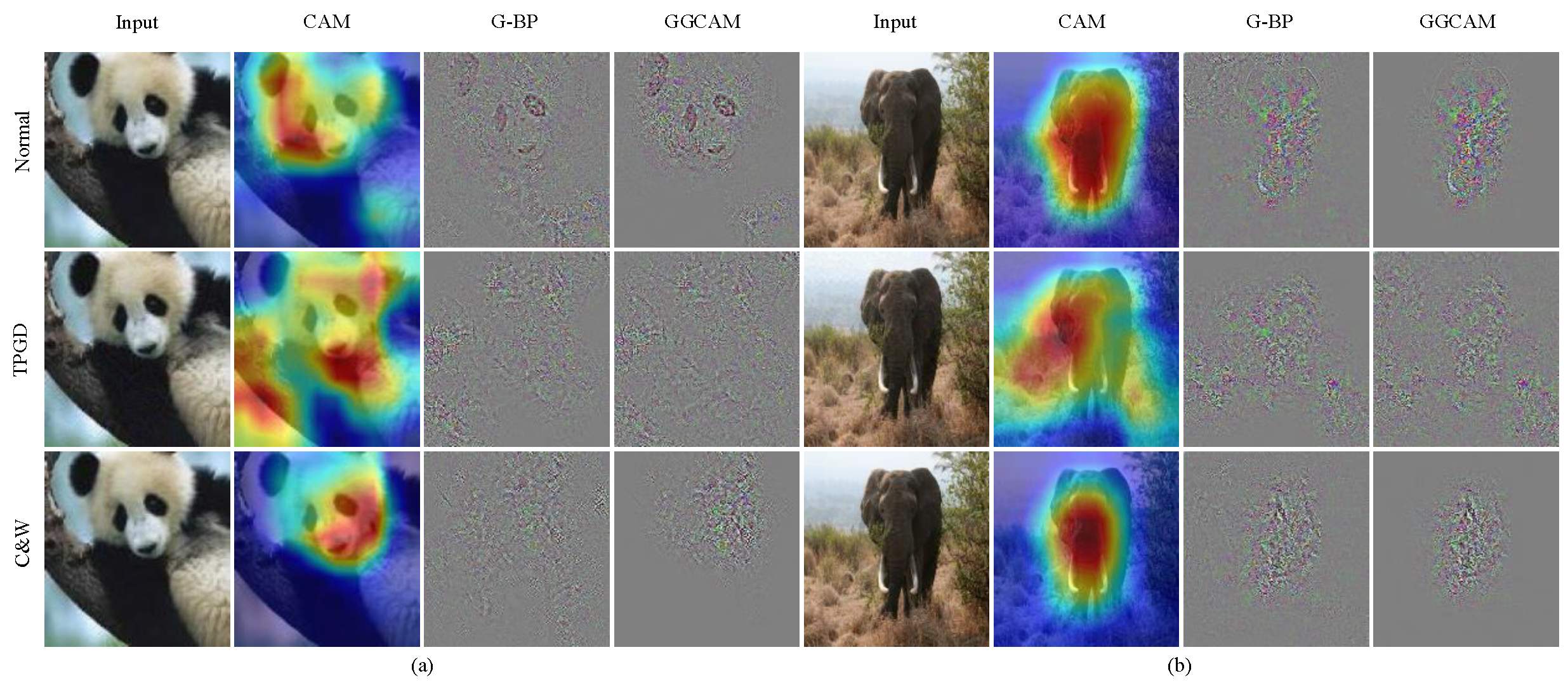
Figure 2 shows that there is a significant difference between the clear and adversarial samples by comparing their attribution maps. Which attribution map has the maximum identification is the key to designing adversarial detection algorithms in this paper. Therefore, we extracted the CAM, G-BP and GGCAM of the two samples in Figure 2, respectively, for comparison, as shown in Figure 3.
We have noted that CAMs exhibit limited differentiation for certain attacks, such as the C&W method. Conversely, guided backpropagation (G-BP) and guided Grad-CAM (GGCAM) demonstrate higher levels of discrimination: the Normal samples display distinct contour features in their attribution maps (see Figure 3: Normal), allowing for rough classification judgments by visual inspection. The introduction of adversarial perturbations, however, leads to a pronounced disruption of these contours in the clear samples (see 
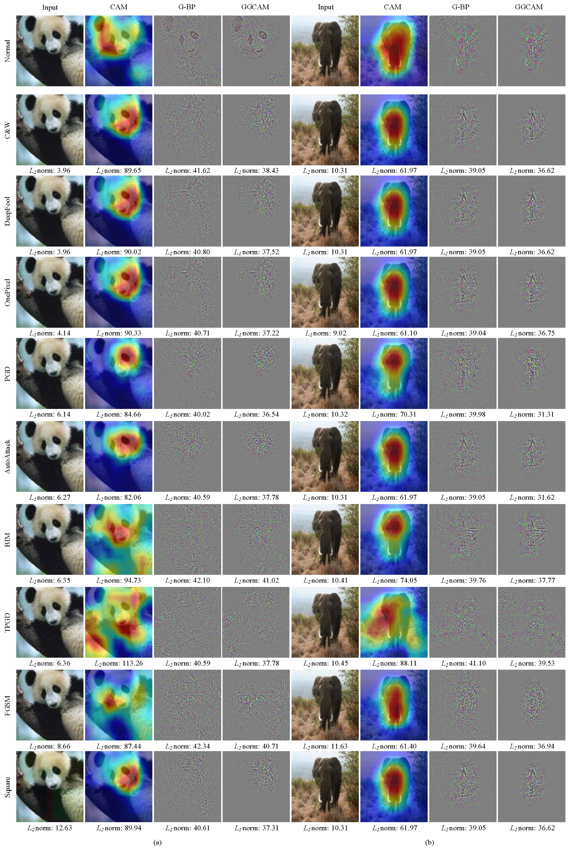
Figure 3: TPGD and C&W), rendering the residual features unintelligible to the human observer. Hence, the disparities in G-BP and GGCAM between the clean and adversarial samples could provide a sufficient basis for detecting adversarial instances. Beyond TPGD and C&W attacks, this study also examines BIM, DeepFool, FGSM, One Pixel, PGD, Square, and Autoattack, employing a total of seven adversarial sample generation methods. The resulting attribution maps are depicted in Figure 4.
Figure 4 shows the comparison of attribution maps between nine adversarial samples and clear samples, among which OnePixel modified one pixel point, and AutoAttack is the adversarial sample generation method, which integrates APGD [50], APGDT [50], FAB [51], and Square [52]. At the same time, we use the L 2 norm, respectively, to calculate the difference between the clear and adversarial samples.
The analysis reveals that the attribution maps for the adversarial samples exhibit discernible alterations following the introduction of adversarial perturbations when compared to clear samples. Notably, the attribution maps measured using the L 2 norm in CAM display the most pronounced differences, characterized by brighter colors and more significant pixel value variations. In contrast, the variations between G-BP and GGCAM are even more apparent, with the contour features of clear samples experiencing substantial disruption. Consequently, the attribution maps generated by CAM, G-BP, and GGCAM demonstrate effective capabilities in identifying adversarial samples.

4. The Proposed Method

The proposed detection method (via attribution maps) can be divided into two parts. The first part is the generation of attribution maps, generating the clear and adversarial samples and turning them into attribution maps through visualization techniques. The second part involves training a binary classifier by using the generated attribution maps to detect adversarial samples. The structure of the two parts is shown in Figure 5.

4.1. The Generation of an Attribution Map

For the first part, we mainly generate the attribution maps of clear and adversarial samples via model visualization technology. Since the CAM method needs to modify the model, Grad-CAM (obtained by improving CAM) does not need to modify the model. Therefore, all the CAMs mentioned in this paper adopt the Grad-CAM method. The following steps outline the specific procedure:
Step 1: In order to compute the gradient of the classification score y c for class c with respect to the feature a k in the convolutional layer, we calculate the partial derivative y c A k . Next, the backpropagation gradient is set to the global average in order to obtain the weight of the feature map, denoted as α k c . As is shown in Equation (2), Z represents the size of the feature A k .
α k c = 1 Z i j y c A i j k
Step 2: Once the weight, α k c , of the feature map has been computed, it is utilized to weigh and combine the feature map activations. This process results in the generation of the activation mapping L c for the class c. The combination of the feature map activations is performed according to Equation (3).
L c = k α k c A k
Step 3: In order to focus solely on the features that positively contribute to class c and disregard negative information that might be associated with other classes, R e L U is applied to calculate L c . This results in the generation of the class activation mapping L C A M c (Equation (4)), which highlights the regions in the input that strongly activate class c.
L C A M c = R e L U ( k α k c A k )
Step 4: The primary distinction between backpropagation and DeconvNet lies in how they handle nonlinearity through the R e L U function. In backpropagation, the threshold value selected during the R e L U operation is based on the feature value of the forward transmission. This is represented by Equation (5), where f I l denotes the input to the R e L U layer. The output of the hidden layer, denoted as f o u t , serves as the threshold value determined by the backpropagation method, as shown in Equation (6). On the other hand, DeconvNet employs the gradient value as the threshold, as depicted in Equation (7). By using the gradient value, DeconvNet adopts a different approach to determining the threshold during the R e L U operation. G-BP, which combines backpropagation and DeconvNet, effectively visualizes the features learned at higher levels of the neural network. By using Equation (8), we obtain G-BP.
f i l + 1 = R e L U ( f i l ) = m a x ( f i l , 0 )
R i l = R i l + 1 · ( f i l > 0 ) , R i l + 1 = f o u t f i l + 1
R i l = R i l + 1 · ( R i l + 1 > 0 )
R G B P i l = R i l + 1 · ( R i l + 1 > 0 ) · ( f i l )
Step 5: The attribution maps of CAM are expanded using linear interpolation, employing interpolation functions with two variables. This process aims to upsample the CAM to match the size of the input sample. Subsequently, the dot product of G-BP and CAM is computed. This calculation is demonstrated in Equation (9), where B denotes the operation of bilinear interpolation. By performing the bilinear interpolation and dot product of G-BP and CAM, GGCAM is obtained.
L G G C A M c = R G B P i l · B ( L C A M c )

4.2. Adversarial Detection Classifier

The task of detecting adversarial samples in UAV-assisted operations demands classifiers that are not only precise but also efficient, considering the UAV constraints on energy, computation, communication, and storage. In the context of UAVs, the models used for such tasks must be optimized for performance while operating within these resource limitations. EfficientNet-B0 [53] stands out as a good choice for UAV vision systems due to its automated model optimization and compound scaling, which allow it to excel in environments where computational resources are at a premium. Its architectural design, consisting of a sequence of mobile inverted bottleneck convolutions (MBConv), convolution layers (Conv), a global average pooling layer (Pooling), and a classification layer (FC), has been tailored for efficiency without compromising accuracy (Table 1). This configuration ensures that high-level performance is maintained even when computational resources are constrained. In contrast to EfficientNet-B0, the widely recognized ResNet50 [54] model serves as a general benchmark to evaluate performance in adversarial detection. While it is a more computationally intensive model known for its deep residual learning framework that eases the training of networks, it offers a comparison point to EfficientNet-B0 in terms of robustness and accuracy. The inclusion of ResNet50 in our comparative analysis provides a broader perspective on how different models perform under the stringent operational conditions of UAVs, allowing us to assess the trade-offs between computational demand and detection capability.
We train our model using a dataset comprising the attribution maps of both adversarial and normal samples. Throughout the training process, we follow the training methodologies and parameter selections, as delineated by Tan et al. [53] for EfficientNet-B0 and He et al. [54] for ResNet50. Our objective is to enable the model to distinguish between these two categories effectively, thereby achieving robust classification performance.

5. Experiment

In this section, we set up three experiments: (1) EfficientNet-B0 as the detector, which verifies the effectiveness of attribution maps. We compare which of the three attribute maps is most suitable for detecting adversarial samples. (2) ResNet50 as the detector, further illustrating that when we choose different classifiers, the attribution maps can also obtain good accuracy. (3) Comparisons with state-of-the-art methods. The experimental part selects the ImageNet validation set as the dataset. Adversarial samples are generated by five attacks, including C&W, BIM, FGSM, PGD, and AutoAttack (APGD, APGDT, FAB, and Square). The code in this paper is implemented via the PyTorch deep learning framework, and we use the TorchAttacks library to generate the adversarial samples.

5.1. Dataset and Models

ImageNet [55] consists of over 1.2 million images across 1000 diverse categories. It is widely used for benchmarking machine learning models in visual object recognition due to its variety of classes and high volume of data. In the context of UAVs, leveraging ImageNet can significantly aid in developing robust object classification algorithms, which are critical for UAV autonomous navigation and operational tasks, such as surveillance or search and rescue. Utilizing ImageNet for adversarial sample detection in UAV data transmission and output processing is crucial because it represents a broad spectrum of real-world scenarios that UAVs may encounter. In this paper, due to the extensive size of the ImageNet dataset, only the verification set consisting of 50,000 images was utilized as the data source.
We selected EfficientNet-B0 and ResNet50 as our classifier models and trained them using the attribution maps of adversarial and normal samples. For EfficientNet-B0, we follow the scaling method proposed by Tan et al. [53]. Additionally, we employ the same RMSprop optimizer with a decay of 0.9 and a momentum of 0.9, alongside a learning rate warm-up and exponential decay, as suggested by Tan et al. [53]. As for ResNet50, following the research of He et al. [54], we utilized a batch normalization momentum of 0.1 and a standard cross-entropy loss function. The model was trained using SGD with momentum, with an initial learning rate set as recommended, which was adjusted following a cosine decay schedule.

5.1.1. Training Sets and Validation Sets

We selected the first 40,000 images in the ImagNet validation set as the normal class. By using the C&W method, these samples were also transformed into adversarial samples and used as an adversarial sample class (not every normal sample can be converted into an adversarial sample). In the training, we selected 20% of the data as the verification set through random sampling, and the remaining 80% of the data was used for training. Table 2 shows the training set and verification set.
In training, we selected 20% of the data in the training set as the verification set through random sampling, and the remaining 80% of the data was used for training. Table 2 shows the training set and verification set.
Finally, our training set contained 32,000 normal samples and 17,616 adversarial samples, and the verification set contained 8000 normal samples and 4403 adversarial samples.

5.1.2. Test Sets

We selected the remaining 10,000 images in the ImagNet validation set as the normal class, and these 10,000 images were converted into five types of adversarial samples by using the C&W, BIM, FGSM, PGD, and AutoAttack methods, which were used as the adversarial samples in the test set. AutoAttack integrates the APGD, APGDT, FAB, and Square attack methods. Table 3 shows the test sets.

5.2. Performance Metrics

The effectiveness of the method is assessed using four key metrics: true-negative ( T N ), true-positive ( T P ), false-positive ( F P ), and false-negative ( F N ). These metrics provide insights into the classification performance. When the positive class in the test dataset is correctly classified as a positive class, it is considered as T P . T N is achieved when a negative class is accurately predicted as a negative class. F N occurs when a positive class is mistakenly classified as a negative class. Conversely, F P happens when a negative class is incorrectly predicted as a positive class. In this paper, the evaluation criteria for the effectiveness of the method are based on the combination of precision (Equation (10)), recall (Equation (11)), and accuracy (Equation (12)).
P r e c i s i o n = T P T P + F P
R e c a l l = T P T P + F N
A c c u r a c y = T P + T N T P + F N + F P + T N

5.3. Experiments Using EfficientNet-B0

As shown in Table 4, the results show that all three attribution maps (CAM, GGCAM, and G-BP) can effectively detect adversarial samples. The average accuracy of CAM is 94.06%, and in comparison with other attribution maps, CAM is lower than GGCAM and G-BP in terms of recall rate, precision, and accuracy. The results show that the difference in the CAM between the normal and adversarial samples is smaller than the other two attribute maps, which contradicts the calculation of the L 2 norm. This indicates that calculating the difference in the attribute maps by using the L 2 norm is not suitable. The average accuracy of GGCAM is 99.38%, which is higher than that of CAM by 5.32%. G-BP has the best effect, with an average accuracy of 99.56%, 0.18% higher than GGCAM. Therefore, the detection of C&W, BIM, FGSM, PGD, and AutoAttack can be realized well via G-BP.

5.4. Experiments Using ResNe50

As shown in Table 5, the detection model is replaced by ResNe50. The results of this experiment are similar to the experiments using EfficientNet-B0. The average accuracy of CAM is 93.03%, which is lower than that of GGCAM and G-BP in terms of recall, precision, and accuracy. When compared with the EfficientNet-B0 used in Experiment 1, the accuracy of CAM decreases by 1.03%, whereas that of GGCAM only decreases by 0.014%. Therefore, using CAM for adversarial sample detection is not stable compared to GGCAM. Meanwhile, all the evaluation indexes of G-BP are higher than CAM and GGCAM. The average accuracy is almost the same as in Experiment 1, even increasing by 0.02%. Therefore, G-BP is better adapted to the detection of adversarial samples.

5.5. Comparisons with State-of-the-Art Methods

Our detection approach was benchmarked against the leading state-of-the-art adversarial detection methods, including kernel density (KD) [39], local intrinsic dimensionality (LID) [56], Mahalanobis distance (MD) [57], LiBRe [58], S-N [59], and EPS-N [59]. By adhering to the experimental protocols established by Zhang et al. [59], our implementation employs the ResNet50 architecture as the foundation for our detector. As indicated in Table 6, our proposed methods exhibit robust performance, surpassing other approaches in average detection success rate across various attack vectors.

5.6. Discussion

The proposed method based on attribution maps can effectively detect C&W, BIM, FGSM, PGD, and other attacks. The average detection accuracy of G-BP can reach 99.58%, indicating that the attribute maps can distinguish clear samples from adversarial samples. We choose the attribution maps as the distinguishing features. This method is feasible and independent of the choice of classifiers.
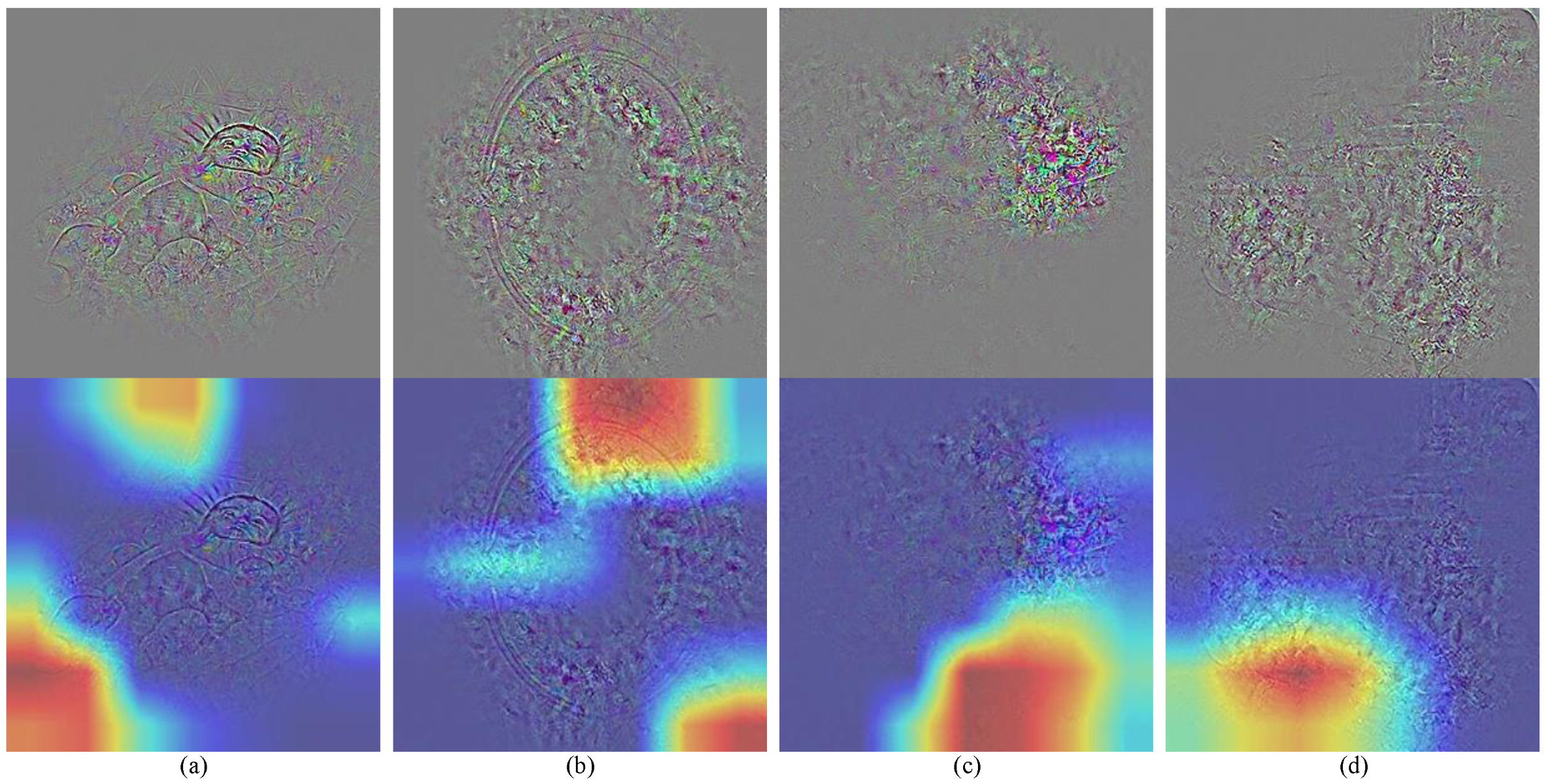
Further analyzing our approach, we focus on error examples in detecting C&W attacks under the Efficientnet-B0 model. In the case of misclassified normal samples (Figure 6), we observe two types of errors. Samples (a) and (b) have relatively clear contours, but the model fails to recognize these features (the highlighted part is not on the contour feature), leading to incorrect classification. Conversely, samples (c) and (d), with fuzzy contours, are also misclassified. This suggests that the model does not consistently extract contour features, leading to the misidentification of these samples as adversarial examples. Improving the steady extraction of contour features in samples will be our focus in future work.
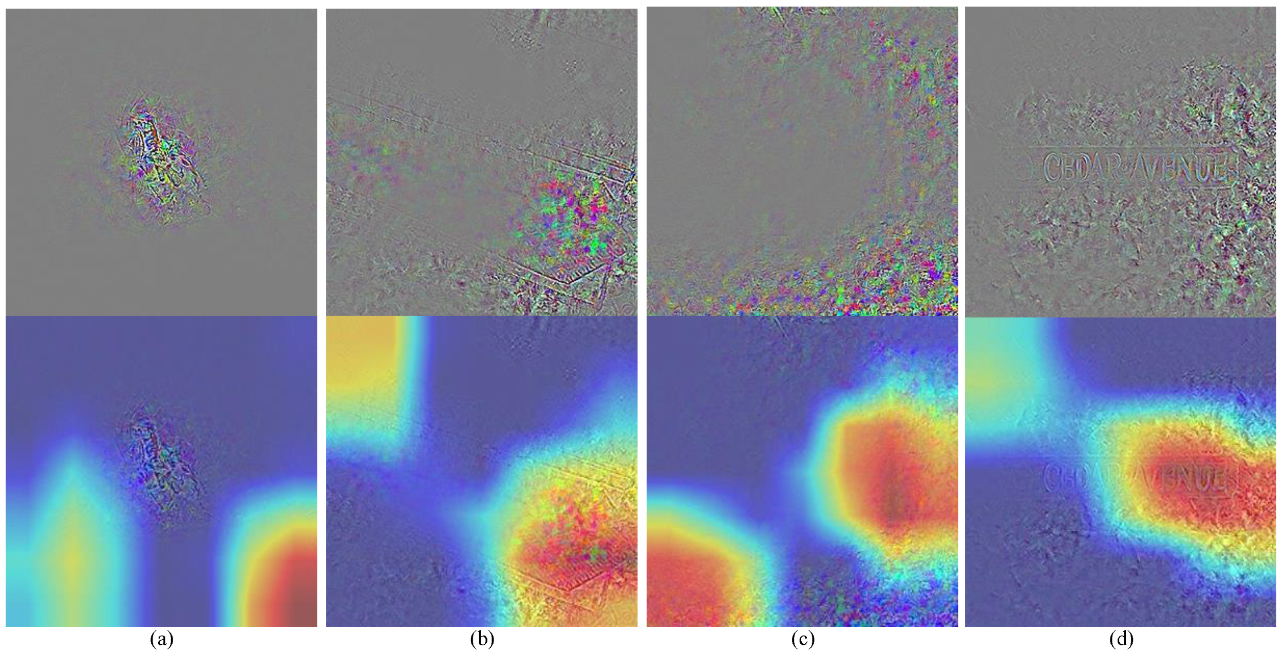
For misclassified adversarial examples (Figure 7), again, we notice two scenarios. In cases (a) and (c), the object’s contour almost disappears due to adversarial perturbations. The model’s regions of interest are not focused on areas with significant gradient changes. This type of error may be attributed to an issue within the model itself. In cases (b) and (d), the partial contours remain visible despite increased adversarial perturbations. A human observer can distinguish objects like a bench or the alphabet. The model focuses on areas with rich contoured features, leading to the misclassification of these adversarial samples as normal. This indicates that the adversarial perturbations added during example generation are not always sufficient.
Our analysis identifies two main issues. The first concerns the stability of contour feature extraction in a small number of samples. As shown in Figure 6c,d, these normal samples’ contour information is not fully captured in the attribution maps. This suggests that our method may struggle with consistently extracting contour features, especially from samples with limited instances. The second issue arises in classes with a small number of samples. Despite the adversarial perturbations, the contour features are not completely disrupted. Figure 7b,d show that only parts of the contours are affected by the perturbations. The remaining intact contour information can lead to misclassification. This underscores the challenge of effectively disrupting the contour features in adversarial samples, particularly in classes with fewer instances.

6. Limitation

While the proposed method—leveraging model visualization technology to generate attribution maps—offers an innovative approach for detecting adversarial examples in UAV vision systems, it also presents certain limitations that warrant further investigation. A primary limitation of our approach lies in the inherent instability of attention-based model visualization methods when extracting features from images. Despite their intuitive appeal and ease of implementation, these methods can sometimes yield inconsistent feature attributions, which may lead to the unreliable detection of adversarial examples. This is particularly problematic in scenarios where decisive image features are subtle or subject to variations in environmental conditions, such as lighting or occlusion.
In order to address this, future work will need to focus on enhancing the stability and consistency of feature extraction within attention mechanisms. This could involve developing more robust attention models that are less sensitive to input perturbations or integrating supplemental techniques that can corroborate and refine the attention-driven feature mappings. Ensuring stable feature extraction is crucial for the dependable deployment of UAV vision systems, where the accuracy of real-time adversarial example detection is paramount.

7. Conclusions

We present a novel method for detecting strong adversarial samples in UAV vision systems using attribution maps. The inclusion of adversarial perturbations causes significant changes in the attribution maps of the samples. By extracting and training a binary classifier on these attribution maps, we can effectively detect multiple types of adversarial attacks. The experimental results demonstrate the superiority of our method. Specifically, our proposed method achieves a detection success rate of 99.58% based on G-BP, surpassing the state-of-the-art methods. Additionally, this method provides the advantage of convenience without requiring modifications to the protected model during the data-input process. It is capable of operating on lightweight models while maintaining high performance. In resource-constrained environments, it serves as an effective safeguard for UAV-assisted IoTs during data collection and transmission processes against adversarial attacks.

Author Contributions

Conceptualization, Z.Z. and Q.L.; Methodology, Z.Z., Q.L., Z.Y., and C.W.; Validation, Z.Z. and Q.L.; Formal analysis, Z.Z.; Investigation, Z.Z.; Data curation, Z.Z.; Writing—original draft, Z.Z. and Q.L.; Writing—review & editing, Z.Z. and S.Z.; Visualization, Z.Z.; Supervision, S.Z.; Project administration, Q.L., S.Z., and C.W.; Funding acquisition, S.Z. All authors have read and agreed to the published version of the manuscript.

Funding

This work was supported by the National Natural Science Foundation of China under Grant 62272089 and the Intelligent Terminal Key Laboratory of Sichuan Province under Grant SCITLAB-30003.

Data Availability Statement

Data are contained within the article.

Conflicts of Interest

The authors declare no conflict of interest.

References

  1. Hadi, H.J.; Cao, Y.; Nisa, K.U.; Jamil, A.M.; Ni, Q. A comprehensive survey on security, privacy issues and emerging defence technologies for UAVs. J. Netw. Comput. Appl. 2023, 213, 103607. [Google Scholar] [CrossRef]
  2. Mason, E.; Yonel, B.; Yazici, B. Deep learning for radar. In Proceedings of the 2017 IEEE Radar Conference (RadarConf), Seattle, WA, USA, 8–12 May 2017; IEEE: New York, NY, USA, 2017; pp. 1703–1708. [Google Scholar]
  3. Rombach, R.; Blattmann, A.; Lorenz, D.; Esser, P.; Ommer, B. High-resolution image synthesis with latent diffusion models. In Proceedings of the IEEE/CVF Conference on Computer Vision and Pattern Recognition, New Orleans, LA, USA, 18–24 June 2022; pp. 10684–10695. [Google Scholar]
  4. Qian, F.; Yue, Y.; He, Y.; Yu, H.; Zhou, Y.; Tang, J.; Hu, G. Unsupervised seismic footprint removal with physical prior augmented deep autoencoder. IEEE Trans. Geosci. Remote. Sens. 2023, 61, 1–20. [Google Scholar] [CrossRef]
  5. Tang, J.; Xiang, D.; Zhang, F.; Ma, F.; Zhou, Y.; Li, H. Incremental SAR automatic target recognition with error correction and high plasticity. IEEE J. Sel. Top. Appl. Earth Obs. Remote. Sens. 2022, 15, 1327–1339. [Google Scholar] [CrossRef]
  6. Wang, L.; Yang, X.; Tan, H.; Bai, X.; Zhou, F. Few-shot class-incremental SAR target recognition based on hierarchical embedding and incremental evolutionary network. IEEE Trans. Geosci. Remote. Sens. 2023, 61, 1–11. [Google Scholar] [CrossRef]
  7. Vint, D.; Anderson, M.; Yang, Y.; Ilioudis, C.; Di Caterina, G.; Clemente, C. Automatic target recognition for low resolution foliage penetrating SAR images using CNNs and GANs. Remote Sens. 2021, 13, 596. [Google Scholar] [CrossRef]
  8. Qian, F.; He, Y.; Yue, Y.; Zhou, Y.; Wu, B.; Hu, G. Improved Low-Rank Tensor Approximation for Seismic Random Plus Footprint Noise Suppression. IEEE Trans. Geosci. Remote. Sens. 2023, 61, 1–19. [Google Scholar] [CrossRef]
  9. Goodfellow, I.J.; Shlens, J.; Szegedy, C. Explaining and harnessing adversarial examples. arXiv 2014, arXiv:1412.6572. [Google Scholar]
  10. Du, M.; Sun, Y.; Sun, B.; Wu, Z.; Luo, L.; Bi, D.; Du, M. TAN: A Transferable Adversarial Network for DNN-Based UAV SAR Automatic Target Recognition Models. Drones 2023, 7, 205. [Google Scholar] [CrossRef]
  11. Huang, T.; Zhang, Q.; Liu, J.; Hou, R.; Wang, X.; Li, Y. Adversarial attacks on deep-learning-based SAR image target recognition. J. Netw. Comput. Appl. 2020, 162, 102632. [Google Scholar] [CrossRef]
  12. Shafahi, A.; Najibi, M.; Xu, Z.; Dickerson, J.; Davis, L.S.; Goldstein, T. Universal adversarial training. In Proceedings of the AAAI Conference on Artificial Intelligence, New York, NY, USA, 7–12 February 2020; Volume 34, pp. 5636–5643. [Google Scholar]
  13. Tramèr, F.; Kurakin, A.; Papernot, N.; Goodfellow, I.; Boneh, D.; McDaniel, P. Ensemble adversarial training: Attacks and defenses. arXiv 2017, arXiv:1705.07204. [Google Scholar]
  14. Burda, Y.; Edwards, H.; Storkey, A.; Klimov, O. Exploration by random network distillation. arXiv 2018, arXiv:1810.12894. [Google Scholar]
  15. Hendrycks, D.; Gimpel, K. Early methods for detecting adversarial images. arXiv 2016, arXiv:1608.00530. [Google Scholar]
  16. Kurakin, A.; Goodfellow, I.; Bengio, S. Adversarial machine learning at scale. arXiv 2016, arXiv:1611.01236. [Google Scholar]
  17. Metzen, J.H.; Genewein, T.; Fischer, V.; Bischoff, B. On detecting adversarial perturbations. arXiv 2017, arXiv:1702.04267. [Google Scholar]
  18. Moosavi-Dezfooli, S.M.; Fawzi, A.; Frossard, P. Deepfool: A simple and accurate method to fool deep neural networks. In Proceedings of the IEEE Conference on Computer Vision and Pattern Recognition, Las Vegas, NV, USA, 27–30 June 2016; pp. 2574–2582. [Google Scholar]
  19. Carlini, N.; Wagner, D. Towards evaluating the robustness of neural networks. In Proceedings of the 2017 IEEE Symposium on Security and Privacy (sp), San Jose, CA, USA, 22–24 May 2017; IEEE: New York, NY, USA, 2017; pp. 39–57. [Google Scholar]
  20. Gong, Z.; Wang, W.; Ku, W.S. Adversarial and clean data are not twins. arXiv 2017, arXiv:1704.04960. [Google Scholar]
  21. Xu, W.; Evans, D.; Qi, Y. Feature squeezing: Detecting adversarial examples in deep neural networks. arXiv 2017, arXiv:1704.01155. [Google Scholar]
  22. He, W.; Li, B.; Song, D. Decision boundary analysis of adversarial examples. In Proceedings of the International Conference on Learning Representations, Vancouver, BC, Canada, 30 April–3 May 2018. [Google Scholar]
  23. Zhang, Z.; Liu, Q.; Zhou, S. GGCAD: A Novel Method of Adversarial Detection by Guided Grad-CAM. In Proceedings of the International Conference on Wireless Algorithms, Systems, and Applications, Nanjing, China, 25–27 June 2021; Springer: New York, NY, USA, 2021; pp. 172–182. [Google Scholar]
  24. Zhou, B.; Khosla, A.; Lapedriza, A.; Oliva, A.; Torralba, A. Learning deep features for discriminative localization. In Proceedings of the IEEE Conference on Computer Vision and Pattern Recognition, Las Vegas, NV, USA, 27–30 June 2016; pp. 2921–2929. [Google Scholar]
  25. Springenberg, J.T.; Dosovitskiy, A.; Brox, T.; Riedmiller, M. Striving for simplicity: The all convolutional net. arXiv 2014, arXiv:1412.6806. [Google Scholar]
  26. Selvaraju, R.R.; Cogswell, M.; Das, A.; Vedantam, R.; Parikh, D.; Batra, D. Grad-cam: Visual explanations from deep networks via gradient-based localization. In Proceedings of the IEEE International Conference on Computer Vision, Venice, Italy, 22–29 October 2017; pp. 618–626. [Google Scholar]
  27. Athalye, A.; Engstrom, L.; Ilyas, A.; Kwok, K. Synthesizing robust adversarial examples. In Proceedings of the International Conference on Machine Learning, Jinan, China, 26–28 May 2018; pp. 284–293. [Google Scholar]
  28. Kurakin, A.; Goodfellow, I.J.; Bengio, S. Adversarial examples in the physical world. In Artificial Intelligence Safety and Security; Chapman and Hall/CRC: Boca Raton, FL, USA, 2018; pp. 99–112. [Google Scholar]
  29. Madry, A.; Makelov, A.; Schmidt, L.; Tsipras, D.; Vladu, A. Towards deep learning models resistant to adversarial attacks. arXiv 2017, arXiv:1706.06083. [Google Scholar]
  30. Dong, Y.; Liao, F.; Pang, T.; Su, H.; Zhu, J.; Hu, X.; Li, J. Boosting adversarial attacks with momentum. In Proceedings of the IEEE Conference on Computer Vision and Pattern Recognition, Salt Lake City, UT, USA, 18–23 June 2018; pp. 9185–9193. [Google Scholar]
  31. Wu, W.; Su, Y.; Chen, X.; Zhao, S.; King, I.; Lyu, M.R.; Tai, Y.W. Boosting the transferability of adversarial samples via attention. In Proceedings of the IEEE/CVF Conference on Computer Vision and Pattern Recognition, Seattle, WA, USA, 13–19 June 2020; pp. 1161–1170. [Google Scholar]
  32. Dong, Y.; Pang, T.; Su, H.; Zhu, J. Evading defenses to transferable adversarial examples by translation-invariant attacks. In Proceedings of the IEEE/CVF Conference on Computer Vision and Pattern Recognition, Long Beach, CA, USA, 15–20 June 2019; pp. 4312–4321. [Google Scholar]
  33. Xie, C.; Zhang, Z.; Zhou, Y.; Bai, S.; Wang, J.; Ren, Z.; Yuille, A.L. Improving transferability of adversarial examples with input diversity. In Proceedings of the IEEE/CVF Conference on Computer Vision and Pattern Recognition, Long Beach, CA, USA, 15–20 June 2019; pp. 2730–2739. [Google Scholar]
  34. Guo, C.; Gardner, J.; You, Y.; Wilson, A.G.; Weinberger, K. Simple black-box adversarial attacks. In Proceedings of the International Conference on Machine Learning, Long Beach, CA, USA, 10–15 June 2019; pp. 2484–2493. [Google Scholar]
  35. Brendel, W.; Rauber, J.; Bethge, M. Decision-based adversarial attacks: Reliable attacks against black-box machine learning models. arXiv 2017, arXiv:1712.04248. [Google Scholar]
  36. Chen, J.; Jordan, M.I.; Wainwright, M.J. Hopskipjumpattack: A query-efficient decision-based attack. In Proceedings of the 2020 IEEE Symposium on Security and Privacy (SP), San Francisco, CA, USA, 18–21 May 2020; IEEE: New York, NY, USA, 2020; pp. 1277–1294. [Google Scholar]
  37. Chen, P.Y.; Zhang, H.; Sharma, Y.; Yi, J.; Hsieh, C.J. Zoo: Zeroth order optimization based black-box attacks to deep neural networks without training substitute models. In Proceedings of the 10th ACM Workshop on Artificial Intelligence and Security, Dallas, TX, USA, 3 November 2017; pp. 15–26. [Google Scholar]
  38. Yang, J.; Jiang, Y.; Huang, X.; Ni, B.; Zhao, C. Learning black-box attackers with transferable priors and query feedback. Adv. Neural Inf. Process. Syst. 2020, 33, 12288–12299. [Google Scholar]
  39. Feinman, R.; Curtin, R.R.; Shintre, S.; Gardner, A.B. Detecting adversarial samples from artifacts. arXiv 2017, arXiv:1703.00410. [Google Scholar]
  40. Ilyas, A.; Santurkar, S.; Tsipras, D.; Engstrom, L.; Tran, B.; Madry, A. Adversarial examples are not bugs, they are features. arXiv 2019, arXiv:1905.02175. [Google Scholar]
  41. Ribeiro, M.T.; Singh, S.; Guestrin, C. “Why should I trust you?” Explaining the predictions of any classifier. In Proceedings of the 22nd ACM SIGKDD International Conference on Knowledge Discovery and Data Mining, San Francisco, CA, USA, 13–17 August 2016; pp. 1135–1144. [Google Scholar]
  42. Chattopadhay, A.; Sarkar, A.; Howlader, P.; Balasubramanian, V.N. Grad-cam++: Generalized gradient-based visual explanations for deep convolutional networks. In Proceedings of the 2018 IEEE Winter Conference on Applications of Computer Vision (WACV), Lake Tahoe, NV, USA, 12–15 March 2018; IEEE: New York, NY, USA, 2018; pp. 839–847. [Google Scholar]
  43. Goyal, Y.; Feder, A.; Shalit, U.; Kim, B. Explaining classifiers with causal concept effect (cace). arXiv 2019, arXiv:1907.07165. [Google Scholar]
  44. Narendra, T.; Sankaran, A.; Vijaykeerthy, D.; Mani, S. Explaining deep learning models using causal inference. arXiv 2018, arXiv:1811.04376. [Google Scholar]
  45. Harradon, M.; Druce, J.; Ruttenberg, B. Causal learning and explanation of deep neural networks via autoencoded activations. arXiv 2018, arXiv:1802.00541. [Google Scholar]
  46. Tabacof, P.; Valle, E. Exploring the space of adversarial images. In Proceedings of the 2016 International Joint Conference on Neural Networks (IJCNN), Vancouver, BC, Canada, 24–29 July 2016; IEEE: New York, NY, USA, 2016; pp. 426–433. [Google Scholar]
  47. Moosavi-Dezfooli, S.M.; Fawzi, A.; Fawzi, O.; Frossard, P. Universal adversarial perturbations. In Proceedings of the IEEE Conference on Computer Vision and Pattern Recognition, Honolulu, HI, USA, 21–26 July 2017; pp. 1765–1773. [Google Scholar]
  48. Zhang, X.; Wang, N.; Shen, H.; Ji, S.; Luo, X.; Wang, T. Interpretable deep learning under fire. In Proceedings of the 29th USENIX Security Symposium (USENIX Security 20), Berkeley, CA, USA, 12–14 August 2020. [Google Scholar]
  49. Zhang, H.; Yu, Y.; Jiao, J.; Xing, E.; El Ghaoui, L.; Jordan, M. Theoretically principled trade-off between robustness and accuracy. In Proceedings of the International Conference on Machine Learning, Long Beach, CA, USA, 10–15 June 2019; pp. 7472–7482. [Google Scholar]
  50. Croce, F.; Hein, M. Reliable evaluation of adversarial robustness with an ensemble of diverse parameter-free attacks. In Proceedings of the International Conference on Machine Learning, Virtual, 13–18 July 2020; pp. 2206–2216. [Google Scholar]
  51. Croce, F.; Hein, M. Minimally distorted adversarial examples with a fast adaptive boundary attack. In Proceedings of the International Conference on Machine Learning, Virtual, 13–18 July 2020; pp. 2196–2205. [Google Scholar]
  52. Andriushchenko, M.; Croce, F.; Flammarion, N.; Hein, M. Square attack: A query-efficient black-box adversarial attack via random search. In Proceedings of the European Conference on Computer Vision, Glasgow, UK, 23–28 August 2020; Springer: New York, NY, USA, 2020; pp. 484–501. [Google Scholar]
  53. Tan, M.; Le, Q. Efficientnet: Rethinking model scaling for convolutional neural networks. In Proceedings of the International Conference on Machine Learning, Long Beach, CA, USA, 10–15 June 2019; pp. 6105–6114. [Google Scholar]
  54. He, K.; Zhang, X.; Ren, S.; Sun, J. Deep residual learning for image recognition. In Proceedings of the IEEE Conference on Computer Vision and Pattern Recognition, Las Vegas, NV, USA, 27–30 June 2016; pp. 770–778. [Google Scholar]
  55. Russakovsky, O.; Deng, J.; Su, H.; Krause, J.; Satheesh, S.; Ma, S.; Huang, Z.; Karpathy, A.; Khosla, A.; Bernstein, M.; et al. Imagenet large scale visual recognition challenge. Int. J. Comput. Vis. 2015, 115, 211–252. [Google Scholar] [CrossRef]
  56. Ma, X.; Li, B.; Wang, Y.; Erfani, S.; Wijewickrema, S.; Schoenebeck, G.; Song, D.; Houle, M.; Bailey, J. Characterizing adversarial subspaces using local intrinsic dimensionality. arXiv 2020, arXiv:1801.02613. [Google Scholar]
  57. Lee, K.; Lee, K.; Lee, H.; Shin, J. A simple unified framework for detecting out-of-distribution samples and adversarial attacks. Adv. Neural Inf. Process. Syst. 2018, 31, 7167–7177. [Google Scholar]
  58. Deng, Z.; Yang, X.; Xu, S.; Su, H.; Zhu, J. Libre: A practical bayesian approach to adversarial detection. In Proceedings of the IEEE/CVF Conference on Computer Vision and Pattern Recognition, Nashville, TN, USA, 20–25 June 2021; pp. 972–982. [Google Scholar]
  59. Zhang, S.; Liu, F.; Yang, J.; Yang, Y.; Li, C.; Han, B.; Tan, M. Detecting Adversarial Data by Probing Multiple Perturbations Using Expected Perturbation Score. arXiv 2023, arXiv:2305.16035. [Google Scholar]
Figure 1. The implementation process of adversarial example attacks. During UAV data acquisition and transmission, attackers add subtle perturbations to the data, generating adversarial examples that can easily mislead the UAV vision system and cause misclassifications.
Drones 07 00697 g001
Figure 2. Samples and their corresponding attribution maps (CAMs). (a,b) are the two samples selected, respectively, where Normal represents the clear samples and their attribution maps, and TPGD and C&W represent the adversarial samples and their attribution maps generated by the corresponding attack method.
Drones 07 00697 g002
Figure 3. Samples and their corresponding three attribution maps (CAM, G-BP, and GGCAM). (a,b) are the two samples selected, respectively, where Normal represents the clear samples and their attribution maps, and TPGD and C&W represent the adversarial samples and their attribution maps generated by the corresponding attack method.
Drones 07 00697 g003
Figure 4. Multiple adversarial samples and their corresponding attribution maps (CAM, G-BP, and GGCAM). (a,b) are the two samples selected, respectively, where Normal represents the clear samples and their attribution maps. The rest are the adversarial samples and their corresponding attribution maps.
Drones 07 00697 g004
Figure 5. The proposed adversarial detection framework based on attribution maps.
Drones 07 00697 g005
Figure 6. Four normal samples (ad) which have been misclassified and their corresponding CAMs.
Drones 07 00697 g006
Figure 7. Four adversarial samples (ad) that have been misclassified and their corresponding CAMs.
Drones 07 00697 g007
Table 1. EfficientNet-B0 baseline network.
StageOperatorResolutionChannelsLayers
1 C o n v 33 × 3 224 × 224 321
2 M B C o n v 1 , k 3 × 3 112 × 112 161
3 M B C o n v 6 , k 3 × 3 112 × 112 242
4 M B C o n v 6 , k 5 × 5 56 × 56 402
5 M B C o n v 6 , k 3 × 3 28 × 28 803
6 M B C o n v 6 , k 5 × 5 14 × 14 1123
7 M B C o n v 6 , k 5 × 5 14 × 14 1924
8 M B C o n v 6 , k 3 × 3 7 × 7 3201
9 C o n v 1 1 & P o o l i n g & F C 7 × 7 12801
Table 2. Training set and validation set.
AttackTypeClassNumber
C&WTrainingNormal32,000
Adv17,616
ValidationNormal8000
Adv4403
Table 3. Test set.
Table 3. Test set.
TypeClassNumber
Test setNormal10,000
C&W4977
BIM9825
FGSM9193
PGD9823
AutoAttack9562
Table 4. Experiments using EfficientNet-B0. We highlight the highest values achieved in each performance metric category in bold.
TypeNumberEfficientNet-B0
CAMGGCAMG-BP
RecallPrecisionAccuracyRecallPrecisionAccuracyRecallPrecisionAccuracy
Normal10,00094.40%95.61%93.37%99.36%99.79%99.43%99.64%99.77%99.61%
C&W497791.30%89.03%93.40%99.58%98.73%99.43%99.54%99.28%99.60%
BIM982594.44%94.31%94.42%99.57%99.35%99.47%99.59%99.63%99.64%
FGSM919395.28%93.99%94.82%98.64%99.30%99.02%98.91%99.61%99.29%
PGD982394.37%94.30%94.39%99.65%99.35%99.51%99.60%99.63%99.62%
AutoAttack956293.60%94.11%94.01%99.51%99.33%99.43%99.55%99.62%99.60%
Average Accuracy94.06%99.38%99.56%
Table 5. Experiments using ResNe50. We highlight the highest values achieved in each performance metric category in bold.
TypeNumberResNe50
CAMGGCAMG-BP
RecallPrecisionAccuracyRecallPrecisionAccuracyRecallPrecisionAccuracy
Normal10,00094.21%95.20%92.96%99.47%99.64%99.41%99.63%99.92%99.70%
C&W497790.46%88.60%92.96%99.28%98.94%99.41%99.84%99.26%99.70%
BIM982591.80%93.97%93.01%99.44%99.46%99.45%99.62%99.62%99.63%
FGSM919392.05%93.60%93.17%98.06%99.42%98.80%99.11%99.60%99.38%
PGD982391.99%93.98%93.11%98.97%99.46%99.22%99.16%99.62%99.40%
AutoAttack956291.68%93.80%92.97%98.82%99.44%99.16%99.70%99.61%99.66%
Average Accuracy93.03%99.24%99.58%
Table 6. Comparisons with State-of-the-Art methods. We have highlighted the two sets of data with the highest detection success rates in bold.
MethodsAttacksAverage Accuracy
FGSMC&WBIMPGD
KD70.99%94.13%97.97%97.20%93.19%
LID89.12%95.28%98.08%97.50%95.82%
MD87.86%96.09%98.35%97.73%95.18%
LiBRe98.89%90.39%92.69%95.30%87.24%
S-N98.28%89.69%72.08%89.74%87.45%
EPS-N99.87%99.78%92.15%99.78%97.90%
CAM(ours)93.17%92.96%93.01%93.11%93.03%
GGCAM(ours)98.80%99.41%99.45%99.22%99.24%
G-BP(ours)99.38%99.70%99.63%99.62%99.58%
Disclaimer/Publisher’s Note: The statements, opinions and data contained in all publications are solely those of the individual author(s) and contributor(s) and not of MDPI and/or the editor(s). MDPI and/or the editor(s) disclaim responsibility for any injury to people or property resulting from any ideas, methods, instructions or products referred to in the content.

