1. Introduction
The decision-making capability is an important attribute, essential for designing autonomous and intelligent systems. Agent-based real-time decision-making based on the data collected by the swarm is proven that can increase the efficiency of the solution and remain robust to dynamic changes and uncertainties. The aim of this work is to examine the efficiency of a decision-making algorithm for swarms compared with other methods, where the decision-making is not existing, and evaluate the methods with a series of metrics in six different scenarios ensuring that the swarm can operate autonomously and safely regarding the inter-agent collisions.
We present a scalable and robust swarm, designed for surveilling a specific area and tracking intruders. The concept is based on that when the swarm starts its operations, it does not have any knowledge about whether intruders exist or not in the monitored area. The intruders spawn at random places in the world during initialization and then there is a fixed time window in which new intruders spawn in the world. The main algorithm behind the swarm’s operation is a stochastic optimization-based decision-making algorithm, responsible for selecting the next task of each agent from a large total of options. The selection criteria are designed so that decision- making is optimized in a system level rather than in an agent level, since we consider that global optimization provides better results for our system. The algorithms needed to support the operation of the swarm are described as implemented.
The key findings of our work are that a swarm with key components such as Task allocation, Collision Avoidance, V2V communications, and V2G communications can perform precisely and robustly a series of tasks in contrast to swarms with no cognitive intelligence, as proven by our experiments. We can observe that when the swarm activates the decentralized decision-making, the effectiveness of the system is increased significantly, as measured by a group of metrics.
Section 2 contains a brief state-of-the-art review focusing on decision-making and task allocation algorithms.
Section 3.1 introduces the UAVs and sensors used in the system. The rest of
Section 3 presents the developed algorithms and the proposed system architecture.
Section 3.7 depicts the tools used to implement and simulate the designed system. In
Section 3.8 and
Section 3.9, the behavior of the simulated intruders and the parameters of the experiment scenarios are presented accordingly. In
Section 4, the metrics used to assess the algorithm and the experiment results are provided, where in
Section 5 we present the key findings of our work. Finally, in
Section 6 we present the conclusions we made conducting these series of experiments.
2. Related Work
The state-of-the-art presents a plethora of different approaches to the use of decision-making in the task allocation problem. According to [
1], the multi-robot task allocation problem is an example of a Discrete Fair Division Problem, as an Optimal Assignment Problem, an ALLIANCE Efficiency Problem or a Multiple Traveling Salesman Problem. The methods to solve the multi-robot task allocation problem can be categorized to be auction based, game theory based, optimization based, learning based and hybrid, as they are listed below.
Auction based: In this type of approach, tasks are offered via auctions, the agents can bid for tasks and the agent with the higher bid is assigned the corresponding task. Each agent bids a value representing the gain of the utility function in case the agent gets assigned that task. The utility function is designed based on the criteria of each problem and takes as inputs the agent’s current state, the task’s description, and the local environment perception of the agent [
2]. The auctioneer might be a central agent, or as it is more common, the auction could be held in a decentralized manner, such as in [
3]. The authors in [
4] address the task allocation problem for multiple vehicles using the consensus-based auction algorithm (CBAA) and the consensus-based bundle algorithm (CBBA), which is a modification of the first one to be applied in multi-vehicle problems. The Contract Net Protocol (CNP) presented in [
5] was the first negotiation platform used in task allocation problems and constitutes the base for numerous task allocation algorithms. CNP was tested in [
6] using a variety of simulation environments to solve the task allocation problem for multiple robots. The authors concluded that because of the interdependency of the tasks in a multi-robot task allocation problem, the original CNP approach does not solve the problem sufficiently.
Game theory based: Game theory-based approaches describe the strategic interactions between the players of a game. Each decision-making agent is considered a player and the game strategy of a player consists of the tasks that the player chose. When the task allocation solution proposed has been optimized globally, all the players will stop changing their strategies, since the optimal outcome has been reached; that condition is called Nash equilibrium. In [
7], the authors present several applications of game-theoretic approaches to UAV swarms. Authors in [
8] proposed a decentralized game theory-based approach for single-agent and multi-agent task assignment for detecting and neutralizing targets by UAVs. In their scenario, UAVs might not be aware of the strategies of other UAVs and a Nash Equilibrium is difficult to achieve. Instead, they used a correlated equilibrium.
Optimization based; Optimization algorithms focus on finding a solution from a set of possible solutions, so that the solution’s cost is minimized, or the solution’s profit is maximized depending on the specific problem’s criteria. Optimization techniques can be distinguished into deterministic or stochastic methods. Deterministic methods always produce the same results for equal inputs, while stochastic methods produce with high probability similar results for equal inputs. Probably the most famous deterministic optimization method used for task allocation is the Hungarian Algorithm (HA) [
9]. The HA attempts to solve the General Assignment Problem (GAP) in polynomial time by maximizing the weights of a bipartite graph. In [
10], the authors approach the task allocation problem as a Vehicle Routing Problem (VRP) in order to solve a multi-agent collaborative route planning problem. In this case, HA is employed after it has been modified to be able to consider constrains, and a detour resolution stage has been added.
A subcategory of stochastic algorithms with great interest for us is the metaheuristics methods which include evolutionary algorithms, bio-inspired algorithms, swarm intelligence, etc. [
11] presents the Modified Distributed Bees Algorithm (MDBA), a decentralized swarm intelligence approach for dynamic task allocation, which shows great results when compared with the state-of-the-art auction-based and swarm intelligence algorithms. In [
12], three different algorithms are presented inspired from Swarm-GAP, a swarm intelligence, heuristic method for the GAP. Authors in [
13] use a genetic algorithm (GA) optimization for decentralized and dynamic task assignment between UAV agents. The task assignment includes an order optimization stage, using GA optimization, for ordering the tasks from a single-agent point of view and a communications and negotiation stage for reallocating tasks between neighboring agents.
Learning based: A commonly used learning-based method is reinforcement learning, a machine learning subcategory. Reinforcement learning algorithms adjust their parameters based on the data gathered from their experiences, to achieve better behaviors. Q-learning is a model free reinforcement learning method, which describes the environment as a Markov Decision Process (MDP). In [
14], a Q-learning implementation for the dynamic task allocation is presented, while the adaptability of Q-learning to uncertainties is showcased in [
15], where it is used for multi-robot task allocation for the fire-disaster response.
Hybrid: Hybrid approaches combine some of the methods listed above to solve the task allocation problem. In [
16], the authors study the Service Agent Transport Problem (SATP), a problem in the family of task-schedule planning problems, using a Mixed-integer linear programming (MILP) of the optimization-based category and an auction-based approach. [
17] proposes an improved CNP technique for solving the problem of task allocation for multi-agent systems (MAS), combining CNP with an ant colony algorithm using the dynamic response threshold model and the pheromone model for the communication between agents. [
18] uses a CBBA-based approach, combined with the Ant Colony System (ACS) algorithm and a greedy-based strategy to solve the problem of task allocation for multiple robots’ unmanned search and rescue missions.
The multi-agent surveillance and multi-target monitoring and tracking problem has been studied by several researchers, and a variety of decision-making techniques have been proposed. A gradient model for optimizing target searching based on beliefs regarding the target’s location is presented in [
19,
20]. They propose a decentralized architecture for the implementation of their algorithm, in which it is assumed that the agents’ belief is globally known across the system, and each agent optimizes its own actions based on the global belief. Authors in [
21] present a decentralized approach, in which UAV agents are organized in local teams, in which the target estimations are communicated. A particle filter is used to track the targets and the estimations are approximated as Gaussian Mixtures using the expectation-maximization algorithm. The leaders of the local teams are responsible for dynamically assigning regions to the team members. A system of UAVs and ground sensors is studied in [
22] for surveillance applications. Targets are detected from both the ground and aerial sensors and UAVs are assigned targets based on a decision-making methodology, so that a multi-attribute utility function is maximized. Partially Observable Markov Decision Processes (POMDPs) have been proposed to model surveillance missions to deal with uncertainties. A methodology to use POMDPs in a scalable and decentralized system is presented in [
23], based on a role-based auctioning method. In [
24], an integrated decentralized POMDP model is presented to model the multi-target finding problem in GPS-denied environments with high uncertainty.
3. Materials and Methods
3.1. Drone Characteristics
3.1.1. Drone Kinematic Model
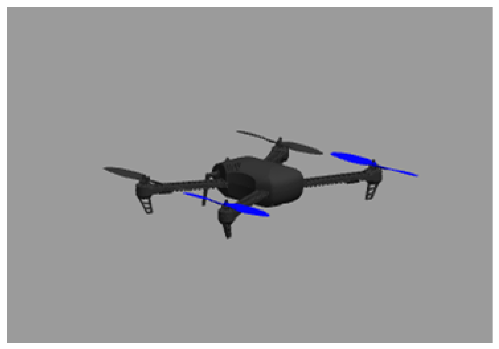
The vehicle used in our tests is a simple quadcopter, shown in
Figure 1, that can be controlled by linear velocity commands in the x, y and z axis. The yaw of the vehicle remains constant with small variations at its initial value, yaw = 0. For all the experiments we assume a constant flight altitude is used.
3.1.2. Sensors
The camera of the agent is directed vertically downwards, as presented in
Figure 2. The camera’s field of view (FOV) for every given moment is a rectangle defined by its height, width, and center. The center of the rectangle coincides with the position of the drone, while the height and width are given by the Equations (1) and (2).
In our case, the flight altitude of the drones was predefined to 20 m for all the simulations and the camera in use has and .
3.2. System Overview
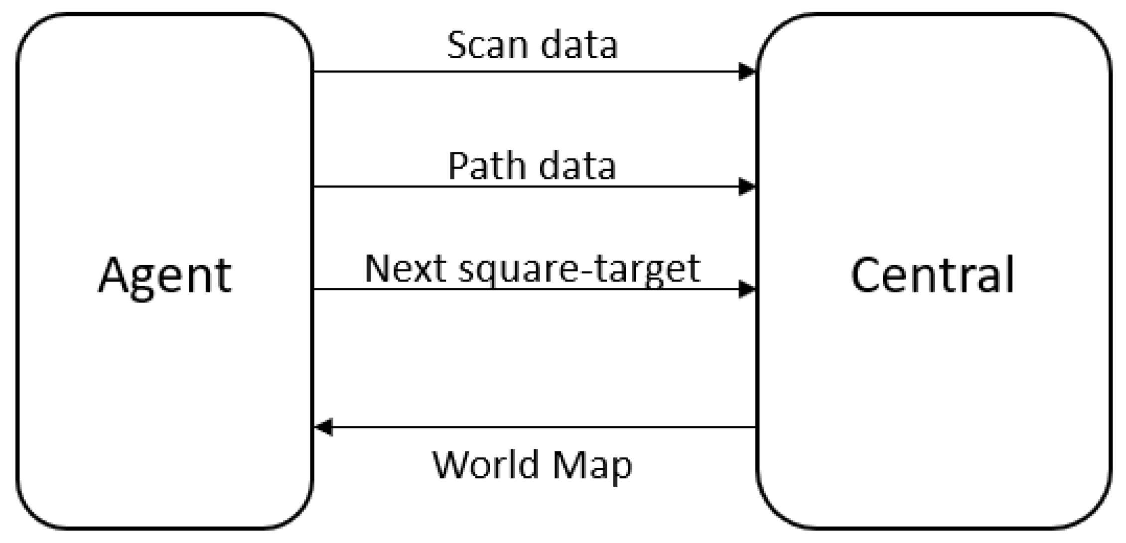
The system is described as a surveillance system with decentralized decision-making capabilities and a central entity acting as a single point of truth. Each agent runs the same code separately and can make its individual decisions. Before each decision is made the agent asks from the central entity to provide him with information about the map/world. That information is gathered in the central entity as each agent sends the data that he is collecting. For every agent an identification number, unique in the swarm, is allocated.
Figure 3 shows the main data exchange between the agents and the central entity.
The messages exchanged between each agent and the central entity are listed below:
From an agent to the central entity:
Scan data: The scan data message includes the identification number of the agent, the number of intruders caught in the square, the number of the intruders detected but not caught while scanning and the 2-D coordinates of the square scanned. The message is sent from the agent to the central entity every time that the agent transitions from the “Scan” mode to the “Go to” mode.
Path data: The path data message includes the identification number of the agent and a list of the intruders that were detected and not caught while moving from the previous target to the next. The message is sent from the agent to the central entity every time the agent transitions from the “Go to” mode to the “Scan” mode, since that is when the agent has completed its path to the new target. Moreover, the path data message will be sent if in the process of following an intruder, another intruder gets detected.
Next-square target: The next target message includes the identification number of the agent and the 2-D coordinates of the next target that the agent selected. That message is sent from the agent to the central entity every time the agent decides on a next target.
From the central entity to an agent:
World map: The world map message is a 2-D matrix with the information about the world, as described in
Section 3.3.
The agents’ behavior consists of three different modes:
Scan: “Scan” mode is activated when the agent is in the boundaries of its square-target. The agent delineates a zig-zag coverage pattern to surveille the whole square-target and check for intruders in that square. If an intruder is detected, then the agent will transit to “Follow intruder” mode. The algorithm used is described in detail in
Section 3.4.
Go to: In this mode, the agent has decided on the next square-target and it moves towards the target in a straight line connecting its current position and the vertex of the square-target that is closer to the current position.
Follow intruder: Independent of the previous mode, when an intruder is detected the agent changes to “Follow intruder” mode. If the agent is already following an intruder, it will keep following the previous intruder and when the intruder is caught the agent will follow the new intruder if the new intruder is still in the agent’s detection range (in the FOV of the agent), otherwise the agent will change to “Go to” mode and move towards the next square-target. In the case that another agent is in a distance that allows him to detect the intruder as well, the agent will drop the “Follow intruder” mode with a probability of 0.1. That characteristic is added to avoid agent congestion over a specific intruder or small group of intruders. The drop probability used may seem too small, but we need to consider that the algorithm runs in a ROS node with a frequency of 5 Hz, so for every second each agent in that situation has a probability of 0.5 to drop the mode.
The agents’ modes and the trigger mechanisms for transitioning between modes are summed up in
Figure 4.
3.3. World Representation
The world is treated as a 2-D grid of 𝑛×𝑛 size, which consists of equal sized squares. A similar approach to discretize the area search problem has been introduced in [
25,
26]. Each square corresponds to one task and each task can be assigned to one agent at any given moment. Each agent is responsible for one task and only when that task is completed or dropped, is when the agent can select a different task. If an agent has selected a task, the central entity flags the square corresponding to that task, so that no other agent is able to select the same task. If two or more agents select the same task simultaneously then the central entity is responsible to inform one of them through a message asking to change their task and repeat the selection process.
The central entity initializes a 2-D matrix containing the grid’s information. The matrix is updated by the central entity based on the data that are received from the agents. When an agent needs to select its next task considering the world information, the agent receives the grid matrix from the central entity. Each node of the matrix includes the following information:
Time of last visit: that contains the time stamp of the last time that the corresponding node was scanned by an agent.
Probability: that expresses the estimated probability of finding an uncaught intruder in that node. The probability is calculated based on the number of intruders that were detected and not caught in that node and in its neighboring nodes. The probability value is initialized at 0.1 for all the nodes (Equation (3)). When a square-target is selected by an agent, its corresponding node’s probability takes a negative value so that no other agent selects that square-target until the current agent has completed its task (Equation (4)). The probability is repaired to its non-negative value when scanning is completed. When scan or path data are received, the probability updates as described at Equations (6)–(10).
Initialize all square probabilities to 0.1:
When a next target message is received for square i as the target assigned to an agent:
When a scan message is received after scanning square i:
The value is computed for every square separately and it is dependent on its distance from the center, since intruders tend to move towards the center and the probability of their next move to be in a square closer to the center has a higher probability. Where is the maximum distance computed from the neighborhood to the target (in our experiments the center of the map). Before it is added to the probability of the square, the value is divided by the sum of all values calculated for the neighborhood so that , where is the neighborhood of square . The size of the neighborhood depends on the speed of the intruders and the size of the squares. In our implementation, the neighborhood consisted of only the squares adjacent to the square , creating a neighborhood of nine squares (3 × 3 square neighborhood), containing the square .
3.4. Coverage Algorithm
The objective of the coverage path planning algorithms is to compute a path that crosses over all points of an area of interest while avoiding obstacles [
27]. As mentioned above, each square of the grid corresponds to an agent’s task. The task to be implemented is for the agent to scan the whole area of the square using a coverage algorithm. Since the main objective of the system is to detect intruders, the scanning is dropped if an intruder is detected, in which case the agent starts following the intruder, activating the “Follow intruder” mode. If no intruder is detected, the task is completed when the area of the square has been scanned.
The scan mode is activated only after the “Go to” mode and the event that triggers that transition is the arrival of the agent at one of the corners of the square to be scanned. Since the FOV of the agent is considered to be a rectangle, the agent does not actually have to be on the edges of the square for them to be scanned. We assume a rectangle smaller than the square and with the same center (the inner rectangle as presented in
Figure 5). The height and width of the rectangle depends on the height and the width of the field of view accordingly and is given by Equations (11) and (12).
where the
and the
represent the height and the width accordingly of the inner rectangle, the
is the length of the edge of each square-target and the
and
are the height and width of the Field Of View of the agents.
The agent moves in the boundaries of the inner rectangle, drawing a zig-zag shaped route. The scanning movement starts with a repeating shift on the x axis until the right-side or left-side (depending on the starting corner) boundary is reached and continues with a shift at the y axis for . The sequence of shifts is repeated with the direction of the shift on the x axis to be inverted for each repetition until the upper-side or downer-side (depending on the starting corner) is reached. When the movement is completed, the agent has visited all the corners of the inner rectangle, and by doing so, it has scanned the whole area of the square.
3.5. Swarm Intelligence—Decision Making
The most important part of the system is the agents’ ability of decision-making to select their next square-target. That is handled by a stochastic algorithm, partially inspired from the ant colony pheromone deposition [
28] idea. The decision-making process is activated when an agent has completed a task and it needs to choose the next square-target as its task. To make its decision, it uses the world information provided by the central entity as a 2-D matrix, containing the probability and time of the last visit of all the square-targets of the grid. The decision-making process is depicted in
Figure 6. The agent first decides if it will stay in its current neighborhood or travel to another neighborhood of the map. That decision is not deterministic, and the agent chooses its current neighborhood with a probability of 0.7, the center neighborhood with probability of 0.06 or a random square-target with probability of 0.24. The ability to travel across the map instead of staying in neighboring squares is added to force the agents to move around the map; this helps to escape local minima by exploring areas of the map that have not been explored recently or detect intruders during the flight and add more information to the world’s matrix. After the agent decides the neighborhood of its next square-target, it needs to select the exact square-target. It computes the margin of every square of the neighborhood based on the Equation (13):
The sum of all the margins of the neighborhood gives the
:
Each margin computed is divided by the
to compute the probability of selecting each square-target.
Finally, the next square-target is selected in a non-deterministic manner and each square-target has a probability to be selected. After the agent selects its next target, it informs the central entity by sending a “Next square-target” message containing its identification number and its selected target.
For the random selection based on probabilities, a simple wheel selection algorithm similar to the one proposed in [
29] was developed. The algorithm is presented in Algorithm 1.
| Algorithm 1. Random selection wheel |
| 1: Choose a random number p in the range [0, 1] |
| 2: Create a list prob_list containing all the probabilities |
| 3: Initialize i as 0 |
| 4: Set prob as prob= prob_list[i] |
| 5: If prob <= p |
| 6: The i element is selected, and the algorithm is terminated |
| 7: Else |
| 8: p = p-prob |
| 9: i++ |
| 10: Repeat from step 4 |
The decision-making algorithm uses the idea of pheromones and evaporation introduced in the ACS, which in our case is implemented by saving the time of the last visit of each square. The agent’s decision is based on how recently the square that it is considering on selecting was visited. In that way, a square that has been scanned recently and hence has higher probability of not having intruders has a lower probability to be picked by the agent. It is clear that in our case the existence of pheromones acts as a suspending factor on visiting an area, which is in contrast to the way that the pheromones are used in the ant colony as described in [
28], where the existence of pheromones increases the probability of an agent to visit the area.
The probability of finding intruders in a square can also be described as an attractive pheromone, which does not obey the evaporation phenomenon. The intruder-related pheromone only increases until the agent scans the corresponding square, and if no intruders are detected it is decreased to its initialization value of 0.1.
We should note here that in the scenario under study the behavior of one intruder is independent on the behavior of the rest of them. Under that assumption, it is not valid to use the information of an intruder that has been caught to predict the behavior of the rest of them. So, the probability of finding an intruder in a square is computed using information regarding only intruders that were detected, but they were not caught. It would be prudent to say that if the behavior of each intruder influences the rest of the intruders, the data concerning the intruders that have been caught would also be useful in determining the probability of finding an intruder in a specific area.
3.6. Collision Avoidance
The most crucial block when dealing with swarms is to ensure that each agent can perform autonomously with safety. Hence, a collision avoidance algorithm is needed to ensure that the agents do not collide on each other. In the literature, a variety of methods exists with many different characteristics and capabilities. A potential field method [
30] was selected both for guiding the agents to a point of interest and for preventing inter-agent collisions. The implemented collision avoidance method is decentralized and it requires for every agent to be aware of the position of the other agents in a distance shorter or equal to 7 m by utilizing V2V communication. The collision avoidance block is enabled only at the “Go to” and “Intruder following” modes. In the “Scan” mode, no conflicts occur, since only one agent could be in the “Scan” mode on a particular square-target at every moment. If two or more agents either in the “Go to” or in the “Intruder following” mode detect a collision in their path, they all act to ensure deconfliction. If one or more agents not in the “Scan” mode detect a possible collision with an agent in the “Scan” mode, the agents that are not in “Scan” mode deconflict while the scanning agent continues its route.
In the “Go to” and the “Intruder following” modes, the objective is similar; navigate to a specific point of interest while avoiding collisions with other agents. The difference between the modes is the type of the point of interest, which is a constant point in the case of the “Go to” mode and a moving ground target in the case of the “Intruder following” mode. Thus, the calculation of the movement commands is conducted in the same way in both modes.
The computed desired velocity of each agent is the sum of attractive velocity and repulsive velocity. The attractive velocity is caused by an attractive force acting on the agent and causing it to move towards the point of interest. The repulsive velocity is caused by a repulsive force acting between agents, which is responsible for not allowing agents to come too close, preventing the possibility of a collision.
The attractive velocity is analyzed at
and
as shown in Equations (16) and (17) and it is dependent on the distance from the target. The coordinates of the target are given as a 2-D point (
,
), as is the position of the agent i (
,
).
The repulsive velocity is also analyzed at
and
and it is calculated from Equations (18) and (19), where the position of another agent j in the detection distance of 7 m is defined as (
,
), and
is the Euclidean distance between the two agents.
The overall desired velocity is expressed in the x, y axes as
and
for each agent i, and it is computed from Equations (20) and (21).
The computed velocity here is the desired velocity of the agent and it is sent to the autopilot, who is responsible for achieving it in a robust and efficient manner. That provides us with the freedom of not having to ensure the continuity of the velocity functions. If the velocities computed here were fed directly to the motors, the continuity of the velocity functions should be ensured, either by computing the velocity indirectly via computing the attraction or repulsion forces, or by adding a maximum velocity change step.
One of the main problems caused by the potential fields family of algorithms is the existence of local minimum that cause the agents to immobilize before they reach their goal [
31]. Local minima could be resolved with three approaches: Local Minimum Removal, Local Minimum Avoidance and Local Minimum Escape (LME) [
32]. Since the environment that we are working in does not contain any static obstacles, the agents could fall into local minimum caused only by the existence of other agents nearby. We choose to resolve local minimum using a local minimum escape method. In the LME approaches, the agents reach a local minimum and then an escape mechanism is triggered to resolve it.
The local minimum detection and resolution is implemented in a decentralized manner by each agent separately. After the agent has computed its desired velocity, it checks if he is trapped in a local minimum. If the agent’s desired velocity is equal to zero (using a threshold near zero) and his attractive velocity does not equal to zero, then the agent is considered trapped. At that point, the agent assumes that all the other agents from which the agent is currently deconflicting are also trapped in the same local minimum. The agent computes the average position of all agents trapped in the same local minimum.
where n_trapped is the number of the agents trapped in that local minimum and i belongs in the set of agents trapped in that local minimum. Each agent i performs a circular motion around the
in an anti-clockwise direction with a constant speed. The agent recomputes its desired velocity in every time step and it continues with the circular motion until it is no longer trapped, in which case it continues with its path.
3.7. Implementation—Simulation
To validate our algorithms and the effectiveness of our system, we performed a series of experiments in simulated worlds. To make our swarm more realistic and applicable to real world scenarios, we decided to use the famous robotics framework ROS [
33]. Using the ROS architecture capabilities, we can add to our system all the desirable aspects for every block we described. The nodes were developed at C++ and python and the ROS version used was ROS melodic. The simulations were conducted using the GAZEBO 7 physics engine [
34], where the PX4 autopilot [
35,
36] was used to control the drones and the selected vehicle was the iris quadcopter, as provided by the PX4.
The central entity is managed by a python script that creates a ROS node is named the central_node, while a ROS node named drone_node was developed in C++ to control the agents. For each agent, an instance of the drone_node runs, given different values for each node. The essential data for each drone_node instance initialization are: the identification number, and the x and y cartesian coordinates of the corresponding agent’s spawn position. The drone_node instances also send control commands with the desired velocity in the x, y and z axis to the PX4 autopilot. The intruders are managed by a python script, which creates a ROS node named intruders_node. The intruders_node is responsible for spawning them and moving them, as described in
Section 3.8, and keeping logs of the metrics presented under
Section 4.2. All of the components described communicate with each other by exchanging messages (publish or subscribe) to specific ROS topics. For the communication of the node developed by our team, special message types were developed to include the exact types of variables needed.
Figure 7 presents the overall system architecture of the implementation of a swarm containing two agents only for demonstration purposes. The figure has been produced from the rqt_graph ROS tool. The nodes are represented by eclipses, while the arrows connecting them represent the topics which they use to exchange messages. The gazebo and gazebo_gui nodes are related to the simulation and the simulation’s graphical user interface. The uav0/mavros and uav1/mavros nodes’ purpose is to transfer information between the ROS environment and the autopilot [
37]. The MAVROS package [
38] enables the data exchange between ROS nodes and autopilots equipped with the MAVLink communication protocol [
39]. The nodes central_node, drone_node0 and drone_node1 were implemented by our team.
3.8. Intruders’ Behavior
In this section, we will present the intruders’ behavior. An intruder in our simulations can be ground moving objects (either people or robots with constant speed and smaller in amplitude to the drone’s speed). An intruder’s goal is to reach the center of the world and stay there for 10 s. The attributes defining the behavior of the simulated intruders are summarized here:
Spawn positions: It is assumed that the world was not being surveilled before the simulation starts, so at the beginning of the simulation, five intruders are spawned at random positions through the world. After that, the intruders are spawned only at the edges of the world, randomly distributed along the four edges of the boundaries of the world.
Spawn time: Spawn time is defined as the time interval between the spawn of two consequential spawning groups of intruders after the simulation starts. In our simulation, that value was constant and equal to 10 s and the size of the spawning group was set to two intruders, so every 10 s, two more intruders were spawned in the simulation.
Movement type: The intruders’ goal is to reach the target, so each intruder’s average movement is on a straight line starting from its spawn position and ending at the target. To recreate a more realistic movement pattern, a stochastic element is added to the constant velocity movement. For every four steps that the intruders make, three of them are the right direction and one of them is in a random direction. After reaching the target, the intruders stay over it for 10 s before they complete their mission. If an intruder completes its mission, it is removed from the simulation.
The intruders are simulated as non-dimensional points with holonomic movement. Since the intruders are assumed to be non-dimensional, inter-intruder collision is not considered.
An intruder is considered caught after it has been tracked by an agent for a predefined tracking time. When an intruder is caught, it is removed from the simulation and the metrics related to the caught intruder are saved.
An intruder is considered alive from its spawn time until it is caught, or it reaches the target.
An intruder is detected from an agent, if the intruder is in the FOV of the agent’s camera.
3.9. Scenario
Six scenarios were designed to test the performance of the algorithm. Each scenario has a different world size and swarm size to evaluate the scalability of the algorithm. The parameters to describe each scenario are listed below:
World size: the size of the simulated world.
Grid size: the size of the grid applied in the world.
Square size: the size of the individual square of the grid depends on the size of the world and the size of the grid and is calculated based on the Equation (23).
Swarm size: the number of the agents of the swarm.
Environment type: an empty environment was selected with no static obstacles that would cause collision risks and visibility constraints.
Simulation duration: the duration of the simulation remained constant for all three scenarios at 33 min in real time simulation.
Intruders spawned: the total amount of intruders spawned during the simulation; that value is constant at 401 intruders for all the scenarios and experiments that were conducted.
Intruders’ average speed: That is computed by dividing the average time that the intruders need to reach the target by the average distance between their spawn position and the target.
Target: The target is defined as the center of the world.
Intruder tracking time: That is defined as the duration of time that an agent needs to track an intruder for the intruder to be considered caught. That was set to 10 s for all scenarios.
Density of agents: That is defined as the number of agents of the swarm divided by the world area.
Table 1 summarizes the different parameters used between the different scenarios. Two sets of scenarios were designed, such that the density of the agents is maintained constant for all scenarios of the set. The size of the surveilled area, the swarm size and the speed of the intruders was changed in every scenario. The speed of the intruders changed proportionally to the area size to maintain the time of the intruders’ life constant and test the algorithms in increasingly difficult scenarios.
In each scenario of the same set, the world size, number of agents and speed of the intruders is increased proportionally, aiming to examine the scalability of our system.
4. Results
In this section, the results from all the experiments conducted are presented.
4.1. Collision Avoidance
A separate scenario was designed for testing the collision avoidance algorithm developed. The scenario is simplified to focus on the collision avoidance. Each agent was given a specific destination point, so that several conflicts would occur in different or in the same position for multiple agents.
Figure 8 and
Figure 9 show the results of a collision avoidance simulation test using four agents. The agents are spawned simultaneously at the vertices of a rhombus and are assigned to go to the opposite vertex. All four of the agents detect the collision and deconflict.
Figure 8 presents the trajectories of the four agents, while they conduct their individual mission and avoid collision with the other three agents. The trajectory of each agent is slightly altered to ensure a collision-free path, but the added cost of the path is not significant, considering that the agents replanned in real-time.
Figure 9 is a diagram of the minimum inter-agent distance for every time step. The minimum measured inter-agent distance decreases significantly around the time value of 20 s, since the agents were in the center area deconflicting at that time, but it remains higher than the minimum allowed inter-agent distance, which for safety precautions was set to 2 m in our experiments.
4.2. Metrics
We propose a set of metrics that can be used to quantify the efficiency of our proposed algorithm regarding the detection of intruders and the area coverage to assess the decision-making process.
Intruder-related metrics:
Number of intruders caught: The sum of the intruders that the agents caught during the simulation run.
Number of intruders reached the target: The sum of the intruders that reached the target during the simulation run.
Average time of intruder’s life: The average alive time of all the intruders during the simulation independently if the intruder was alive or not at the end of the simulation, measured in seconds.
Average time of intruder’s life for caught intruders: The average alive time of the intruders which were caught during the experiment, measured in seconds.
Average time of intruder’s life for reached intruders: The average alive time of the intruders that successfully reached the target, measured in seconds.
Decision metric: The decision metric is the average time interval between two successive decisions of one agent. It is measured in seconds.
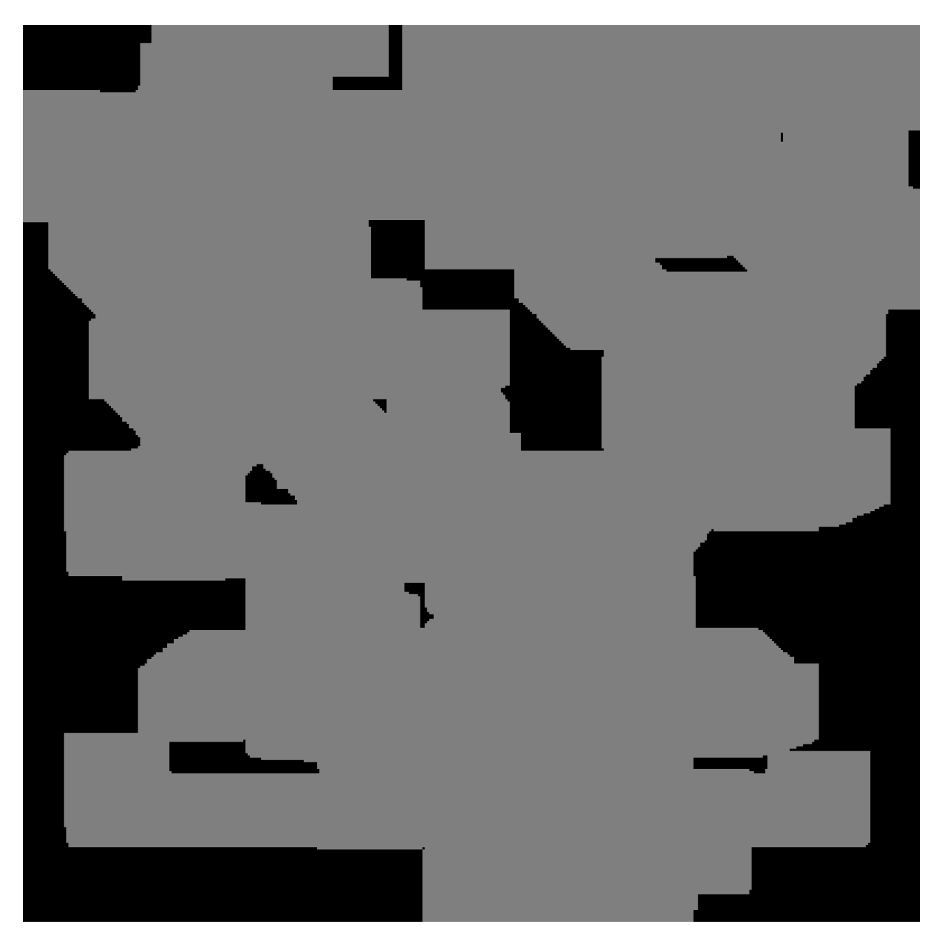
Coverage metric: The coverage metric is defined as the percentage of the world that has been covered by the swarm. That metric is initialized every
seconds, where
was set to
for our simulations. That metric is an indication of how effectively the area of interest is covered, but it is of less importance than the intruder’s metrics in our case. We can easily understand that this metric ensures us about the correct functionality of the decision-making process.
Figure 10 shows an example of the coverage metric.
4.3. Competing Algorithms
Three competing surveillance methods were developed and implemented to compare their results with our method.
Map division: The area of interest is divided into n rectangles, where n is the number of the agents of the swarm. Each agent undertakes the surveillance of one of the rectangles. The first action of each agent is to compute their rectangle and to move to it. After that, each agent changes to mode “Scan” and starts scanning the rectangle using zig-zag-like coverage. If the agent detects an intruder, it changes to “follow intruder” mode. When the intruder is caught, the agent carries on with scanning if the agent is in the boundaries of its rectangle. Otherwise, the agent changes to the “Go to” mode until it is in the boundaries of its rectangle and then changes to “scan” mode. Collision detection and avoidance is only activated if the agent is out of the boundaries of its rectangle since the rectangles do not overlap and there is no risk of collision when all the agents are the boundaries of their own rectangle. Algorithm 2 is used to divide the map into squares by setting the number of columns, nc, and rows, nr.
| Algorithm 2. Map division |
| 1: Set n the number of drones in the swarm |
| 2: If the square root of n is an integer |
| 3: root = nc = nr = |
| 4: Else |
| 5: nc = round () |
| 6: nr = 1 |
| 7: While nc > 0 and n% round(root) ! = 0 |
| 8: nc = round ( |
| 9: nr = |
| 10: root = root -−1 |
After the number of rows and columns is computed, each drone calculates the vertices of its square based on its ID, the world size, the coordinates of the center of the world and the computed number of rows and columns.
Random decision: In this scenario, the agent’s modes are the same as in our proposed algorithm, but the swarm intelligence has been removed. The agents do not make decisions based on the world information and the central entity does not exist. The agents select the next square-target at random each time.
Static cameras: In this scenario, the agents take off and hover statically over a specific predefined position, different for each agent acting as static cameras. They are not allowed to follow intruders.
Figure 11 presents the configuration of the static cameras for each scenario.
4.4. Experiment Results
This section includes the experimental results of the simulations conducted to assess the efficiency of our proposed algorithm and to compare the results with the competing algorithms. Each experiment was run five times and the results were averaged to be presented here. The number of intruders reached the target and the number of intruder-caught metrics are the most indicative of all the metrics used to assess the algorithms, since preventing the intruders from reaching the target is the main objective of the system.
In
Figure 12, the results are presented for our first group of tests, where we maintain a UAV density of 25 square-targets per UAV. To keep the density constant, the area is increased linearly with the number of UAV agents. On the first graph of
Figure 12, the results for 4 UAVs indicate that our decision-making algorithm outperforms all other algorithms, by letting just 10 intruders to reach their target. The random decision algorithm and map division algorithm perform closely to each other with 35 and 40 intruders reaching the target, respectively, and lastly, the static camera approach failed to catch most of the intruders, as 328 reached their target. We can observe that the proposed algorithm performs almost 350% better for the number of intruders reaching the target metric than the second best, which is the random decision.
Our decision-making algorithm was able to catch 364 intruders, 22 more than the random decision algorithm and 26 more than the map division approach, by allocating resources in intruders’ clusters, mostly close to the map center, where intruders converge. This in return increased the average alive time of caught intruders to 124 s, 22 more versus both the random decision and map division approaches. In this scenario, the system is stressed due to the low number of UAVs in comparison to the number of intruders, which results to most of the time being spent following intruders instead of actively searching. When 8 and 16 UAVs are used as shown in the second and third graphs of
Figure 12, we see that the decision-making algorithm performs similarly to the random decision one, with the map division approach performing a bit worse. The similar performance of the first two algorithms is explained by the low density of 25 square-targets per UAV, which in return minimizes the benefits of decision-making since a random approach still has a high chance of finding intruders. In all tests, static cameras proved inefficient and map division fell behind likely due to the inability of the system to migrate resources to hotspots.
In
Figure 13, results are presented for the second experimental set, while we maintain a UAV density of 56 square-targets per UAV, more than twice higher than in set 1. In the first graph of
Figure 13, the results for scenario 1 of set 2 are presented for four UAVs. The decision-making algorithm outperforms the three competing algorithms, but the performance is still rather poor, letting 33 intruders reach their target. The random decision algorithm and map division algorithm perform closely with 90 and 84 intruders reaching the target, respectively, and lastly, the static camera approach failed to catch most of the intruders, as 319 reached their target. The decision-making algorithm was able to catch 337 intruders, 48 more than the random decision and map division algorithm, which performed equally in this metric, while static cameras caught only 36 intruders. The problem described in the previous set of scenarios when four UAV agents are involved, is furtherly amplified by the increase in map size to achieve 56 square-targets per UAV. The average alive time of the caught intruders is 155 s, 42 more versus the random decision and 23 more versus the map division approach. These critical metrics show the worst performance than the first group of tests, attributed to the increased map size while still using four UAV agents.
When 8 and 16 UAV agents are used, as shown in the second and third graphs of
Figure 13, the benefits of decision making are clearer when compared to other approaches as the higher amount of squares per UAV agent allows for a significant chance of a random decision being wrong. When 8 UAVs are involved, 20 intruders reached their target using the decision-making algorithm, 46 for random decision, and 43 for map division, which performed once again roughly equally. Static cameras once more proved to be significantly worst in these tests, as 302 intruders reached their targets. The decision-making system caught 355 intruders, 26 more when compared to random decision and 28 more when compared to map division. The trend continues for 16 UAVs with decision making having a large lead, catching 350 intruders, and missing just 24 intruders. In this case, the random decision proved better than map division, as 40 intruders reached their goal and 337 were caught, while the results were 58 and 321, respectively, for map division. Map division underperforms, likely due to the inability of the system to migrate resources to hotspots.
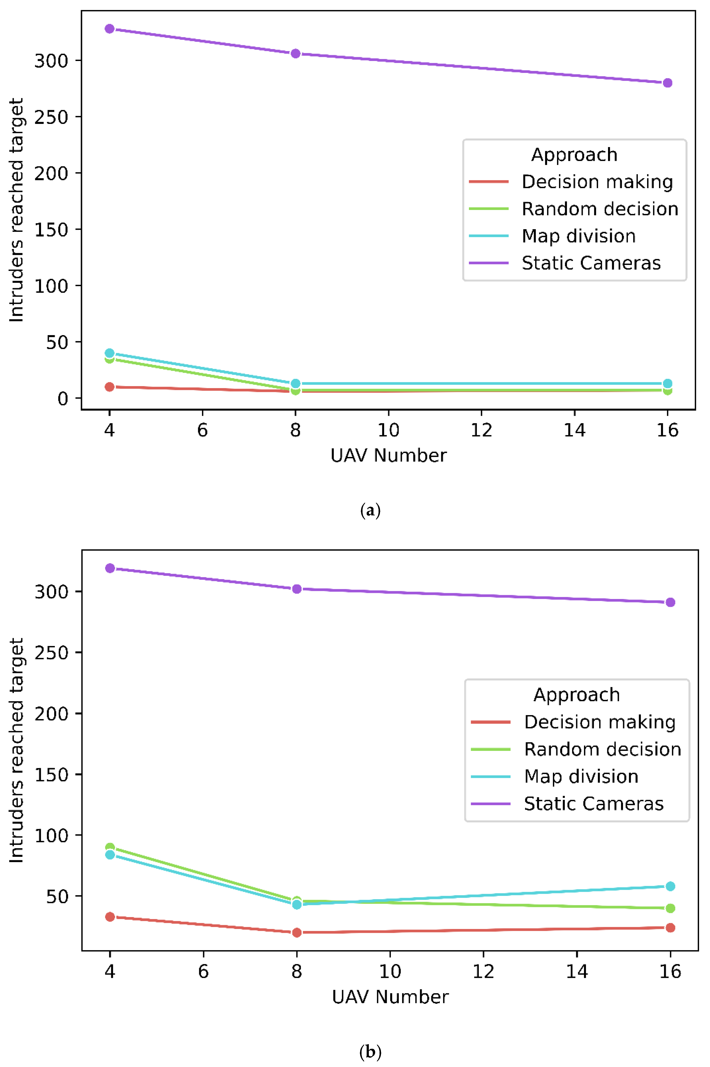
Figure 14 focuses on the number of intruders that reached the target for the different scenarios of each set. Plot (a) shows that the number of intruders to reach the target is relatively stable across the scenarios of set 1 and maintained in low values for the decision-making approach. That indicates that the system’s performance fits the specific density used in set 1 of one UAV agent per 25 square-targets. The random decision and map division approaches demonstrate similar results to the decision-making approach as the size of the swarm increases, indicating that the number of UAVs is enough for monitoring the given area, even for systems with no decision-making capabilities. Plot (b) presents the same metric for the second experimental set. In this case, the density of UAVs per square-target is lower and the advantage of using agents capable of decision-making is clearer, as the proposed decision-making approach outperforms the three competing approaches.
In all of the experiments presented above, the intruder speed was increased proportionally to the world’s dimensions in an attempt to keep the difficulty equal in that regard. In
Figure 15, the performance results of an extra scenario are presented for the case when 16 UAVs are deployed and 56 square-targets are assigned to each UAV, such as in the case of the scenario 3 of set 2. In this experiment, the speed of intruders was not adjusted to the world’s dimensions, and it had the value of 0.28 m.
. Intruders were not able to reach their target for the decision-making, random decision and map division approaches, and the average duration of their life is comparable for the three approaches. The excellent performance of the three approaches was probably caused by the long life-time required for an intruder to reach the target in this scenario. It seems that the increase in the world size would create a severe advantage for all approaches, and the results would not give a clear comparison between the approaches. Based on those results, an adjustable intruders’ speed has been selected for all the experiments presented above.
Table 2 sums up the decision-making metric average results for the six scenarios. The time interval between two subsequent square-target selection is shorter for the decision-making algorithm than for the random decision that is explained because the random decision allows the agents to travel across the map in each decision, while the decision-making algorithm urges agents to stay in their neighborhoods with a large probability. By maintaining the decision-making metric small, the system will have a quicker reaction to new intruder data.
Table 3 presents the average of the coverage metric for each scenario and implementation. It is noticeable that the random decision implementation offers a larger area coverage for each scenario. Before extracting any conclusions concerning the efficiency of the algorithms based on that metric, it should be noted that larger area coverage does not result to more efficient area coverage. The reason behind the lower area coverage provided by the decision-making algorithm is that agents tend to cluster over areas with high intruder density, which enables the detection of a larger amount of intruders.
We can see in
Figure 16 that the swarm manages to cover a big size of the area to be surveilled and is not biased in the selection of the next grid by selecting only certain areas of the world, resulting in the even distribution of the selection across the map based on the collected information. It is clear that of the two sequential coverage measurements in
Figure 16a,b, that the swarm covers all the map and does not show preference to specific areas.
Even though mostly two of the proposed metrics (the Number of intruders caught, and the Number of intruders reached the target) are used for the efficiency assessment of the algorithms, the rest of the metrics are of importance as well. All the proposed metrics are good indicators of how well tuned the decision-making algorithm is. It is a subject of further research to determine the exact equations to compute all the algorithm’s parameters based on those metrics.
6. Conclusions
We present a system consisting of multiple UAV agents, designed for area surveillance and intruder monitoring. In addition to the state-of-the-art decentralized decision-making algorithm that is proposed, the supportive algorithms were also designed and implemented. The system was originally fine-tuned for a scenario with a swarm of four agents and a world size of 100 m × 100 m (scenario 1 of set 1). The results for this scenario are 363.6 intruders caught over the 401 intruders introduced in the world for our decision-making algorithm and 342.2, 337.6 and 24.4 accordingly for the random decision, map division and static cameras implementations. The average value of the intruders reaching the target for this scenario is 9.8 for our decision-making algorithm and 35.4, 39.4 and 328 accordingly for the random decision, map division and static cameras implementations. Overall, the system was tested in two experimental sets, maintaining a constant density of UAV agents per monitored area across the set. Each set included three scenarios, varying in the size of the swarm, the size of the world, and the intruders’ speed. In all six scenarios, the proposed algorithm demonstrates superior results to the three competing systems. The proposed approach demonstrated comparable results across the three experiments of each set indicating that the UAV density is a stronger factor in the system’s performance than the size of the monitoring area. That shows the scalability characteristic of the system. One exception to the stable performance of the system was identified for the first scenario of the second set, in which the system seems to have reached its limits, as the number of the intruders and their relatively high speed caused agents to chase intruders for most of their operational time, and the decision-making algorithm demonstrated a lower performance. As a result, we conclude that the existence of cognitive intelligence in a swarm is crucial and produces much higher situational awareness as opposed to the cases where the swarm is selfish and each agent act on his own without utilizing any shared information. The overall system was tested in real time simulations and demonstrated an improvement up to 350% when compared with similar systems that lacked the decision-making ability. Though the proposed decision-making algorithm was designed to be decentralized, the presented communication scheme of this work requires communication with a central agent, as the necessary processing power of the described central agent is very low, and that processing load may be allocated to the agents. Future work shall include the implementation of a decentralized communication layer for the world map data.
The key contribution of the present paper is the description of a decentralized decision-making algorithm designed for area monitoring and intruder tracking by a swarm of UAVs. The overall system was implemented to support the testing of the algorithm, including collision avoidance and area coverage algorithms. The system was developed in ROS and simulated in GAZEBO with swarms of up to 16 quadcopters. Experiments of this study included intruders incapable of planning to avoid UAV agents. Future research shall focus on adding strategy to the intruders’ behavior and more elaborate models of estimating the intruders’ near-future locations. It is of interest to investigate how the system will perform when faced with smarter intruders upgraded with self and group strategies to achieve their goal of reaching the target. We believe that the system’s performance can be enhanced by the addition of alternative stochastic models describing the probability of an intruder’s presence, especially in the case of intruders capable of strategic planning and collaboration. Finally, future research will also include the development of object detection, target tracking and localization techniques for detecting and following the intruders. This will allow us to study the uncertainties added during intruder detection and localization and may demonstrate some of the limitations of the system.

 ,
, 


