Article

Investigating a Fractal–Fractional Mathematical Model of the Third Wave of COVID-19 with Vaccination in Saudi Arabia

1
Department of Mathematics, College of Arts & Sciences, Najran University, Najran 66462, Saudi Arabia
2
Department of Mathematics and Statistics, College of Science, University of Jeddah, Jeddah 21589, Saudi Arabia
3
Laboratory of Mathematics Modeling and Applications, University of Adrar, Adrar 01000, Algeria
4
Laboratory of Applied Mathematics, Kasdi Merbah University, Ouargla 30000, Algeria
*
Author to whom correspondence should be addressed.
Fractal Fract. 2024, 8(2), 95; https://doi.org/10.3390/fractalfract8020095
Submission received: 22 December 2023 / Revised: 26 January 2024 / Accepted: 28 January 2024 / Published: 2 February 2024

Abstract

:
The severe acute respiratory syndrome coronavirus 2 (SARS-CoV-2) is responsible for coronavirus disease-19 (COVID-19). This virus has caused a global pandemic, marked by several mutations leading to multiple waves of infection. This paper proposes a comprehensive and integrative mathematical approach to the third wave of COVID-19 (Omicron) in the Kingdom of Saudi Arabia (KSA) for the period between 16 December 2022 and 8 February 2023. It may help to implement a better response in the next waves. For this purpose, in this article, we generate a new mathematical transmission model for coronavirus, particularly during the third wave in the KSA caused by the Omicron variant, factoring in the impact of vaccination. We developed this model using a fractal-fractional derivative approach. It categorizes the total population into six segments: susceptible, vaccinated, exposed, asymptomatic infected, symptomatic infected, and recovered individuals. The conventional least-squares method is used for estimating the model parameters. The Perov fixed point theorem is utilized to demonstrate the solution’s uniqueness and existence. Moreover, we investigate the Ulam–Hyers stability of this fractal–fractional model. Our numerical approach involves a two-step Newton polynomial approximation. We present simulation results that vary according to the fractional orders ( γ ) and fractal dimensions ( θ ), providing detailed analysis and discussion. Our graphical analysis shows that the fractal-fractional derivative model offers more biologically realistic results than traditional integer-order and other fractional models.

1. Introduction

The onset of the novel severe acute respiratory syndrome coronavirus 2 (SARS-CoV-2) in late 2019 marked the beginning of a global pandemic that profoundly impacted all aspects of human society. Coronavirus disease-19 (COVID-19) has caused widespread illness, loss of life, economic disruptions, and a significant strain on healthcare systems worldwide. Typical symptoms include fever, cough, fatigue, and difficulty breathing, with the disease being more severe for the elderly and those with underlying chronic conditions.
Mathematical modeling has been instrumental in understanding and combating the pandemic. Among the various models, fractal–fractional modeling stands out, shedding light on the intricate transmission patterns of COVID-19. Rooted in fractal geometry and fractional calculus, this approach captures the self-similar patterns in the virus’s spread. It provides a mathematical framework mirroring the nonlinearity and variability observed in actual epidemic data [1,2,3]. Multiple mathematical frameworks have been developed and scrutinized to understand COVID-19 transmission globally. For instance, Ref. [4] proposed a model incorporating lock-down measures for COVID-19. Additionally, the impact of unidentified cases was examined in [5] through a distinct mathematical framework. Specific preventive strategies’ influence on the trajectory and management of COVID-19 in Pakistan was detailed in [6]. Furthermore, Ref. [7] considered the environmental dissemination of the virus in a transmission model focused on a Saudi Arabian case study. Notably, the majority of COVID-19 models rely on integer-order derivatives, which may sometimes inadequately represent certain realistic features.
To overcome these challenges, fractional-order derivatives serve as a valuable tool for understanding disease dynamics, providing additional crucial insights. Models using fractional-order mathematics inherently possess memory properties, offering a more suitable approach to characterize epidemic models. The application of fractional-order derivatives in disease dynamics has been explored in works such as [8,9] and related studies.
In recent times, a surge in the development of fractional-order mathematical models aimed at unraveling the dynamic behaviors of the emerging COVID-19 pandemic has been observed. For instance, Ref. [10] presented a COVID-19 model utilizing Caputo fractional operators, focusing on pandemic data from China. Additionally, a model centered on the fractional Atangana–Baleanu operator was introduced to depict the spread of COVID-19. The analysis prompted a discussion on the represented transmission dynamics and their implications for societal infection patterns [11].
In [12], a model based on the S E I R compartment, utilizing non-singular derivatives, examined the progression of COVID-19 in India. The q-Homotopy analysis transform method was employed for solution derivation. Additionally, Ref. [13] introduced dynamic and numerical approximations for an arbitrary-order COVID-19 system, considering three specific derivative operators. Furthermore, Ref. [14] advanced a fractional model within the Atangana–Baleanu–Caputo context, emphasizing the advantages of non-integer orders over integer orders.
This paper aims to explore the transmission dynamics of COVID-19 in Saudi Arabia by employing a compartmental model grounded in Caputo fractional-order derivatives. The progression of infectious individuals is categorized into reported cases (identified through COVID-19 testing) and unreported cases (those who have not undergone testing). As a result, the initial S A I R (Susceptible-Exposed-Infected-Recovered) model with vaccination evolves into S V A I u I r R (Susceptible-Vaccinated-Exposed-Asymptomatic infected-Symptomatic infected-Recovered) (refer to Figure 1 for the virus’s dynamics in each compartment). Utilizing actual data from Saudi Arabia, we estimate the parameter values for the suggested mathematical model of COVID-19.
The paper’s structure is outlined as follows: Section 2 presents preliminary findings utilized throughout the paper. Section 3 details the Caputo fractional-order model and the estimation methodology. Section 4 delves into fundamental model analysis, including solution existence and uniqueness, the basic reproduction number indicating disease transmissibility, and the stability of model equilibria. Section 5 introduces the numerical scheme for the FF model. Numerical simulations and model discussions are covered in Section 6, and Section 7 concludes with final observations.

2. Preliminary Results

This section gives some basic definitions and fundamental concepts related to fractional and fractal–fractional calculus and generalized Banach spaces; for more details, we suggest Refs. [1,15,16,17].
Definition 1.
Recall that the Riemann–Louiville fractional integral of order γ of a function f : R + R is defined by
I 0 , t γ f ( t ) = 1 Γ ( γ ) 0 t ( t s ) γ 1 f ( s ) d s ,
where γ R + is the order of integration, and Γ ( γ ) = 0 + e t t γ 1 d t is the Gamma function.
Definition 2.
The Caputo fractional derivatives of order γ R + of a function  f : R + R are defined as
  0 C D t γ f ( t ) = 1 Γ ( n γ ) 0 t ( t s ) n γ 1 f ( n ) ( s ) d s
Here, n = [ γ ] + 1 , where [ γ ] denotes the integer part of γ from the set of positive real numbers R + .
The Caputo derivative and the Riemann–Liouville integral adhere to the subsequent properties:
1.  
  0 C D t γ ( I 0 , t γ f ( t ) ) = f ( t ) ;
2.  
For   0 C D t γ ( C ) , where C is an element of the real numbers R , the result is zero;
3.  
I 0 , t γ (   0 C D t γ f ( t ) ) = f ( t ) k = 0 n 1 f ( k ) ( 0 ) k ! t k ;
4.  
Provided that γ satisfies 0 < γ < 1 , it follows that I 0 , t γ (   0 C D t γ f ( t ) ) = f ( t ) f ( 0 ) .
Definition 3
([15]). Consider a function ϱ that is differentiable within the open interval ( a , b ) . Assuming ϱ possesses fractal differentiability of order θ over this interval, we can then define its fractal–fractional derivative (abbreviated as FF derivative) of order γ following the Caputo approach, characterized by a power law.
  a C D t γ , θ ϱ ( t ) = 1 Γ ( n γ ) a t ( t τ ) n γ 1 d n ϱ ( τ ) d t θ d τ n 1 < γ , θ n , n N .
where
d ϱ ( t ) d t θ = lim s t ϱ ( s ) ϱ ( t ) s θ t θ .
Lemma 1.
Equation (3) can be expressed in the following manner:
  0 C D t γ , θ ϱ ( t ) =   0 C D t γ ϱ ( t ) 1 θ t θ 1 , where , n = 1 , a = 0 .
The Perov fixed point theorem is used to demonstrate the existence and the uniqueness. To proceed, we shall explore several key topics from generalized Banach spaces that are linked to this theorem.
Definition 4.
Let E be a vector space over K = R or C . A generalized norm on E is a map:
· G : E [ 0 , + ) n G = 1 n ,
with the following characteristics:
(i)
For all E , if G = 0 R + n , then = 0 E ;
(ii)
a G = | a | G for all E and a K ;
(iii)
+ ω G G + ω G for all , ω E .
The pair ( E , · G ) is called a generalized normed space. Moreover, ( E , · G ) is called a generalized Banach space (in short, GBS) if the vector-valued metric space generated by its vector-valued metric δ G ( 1 , 2 ) = 1 2 G is complete.
Definition 5.
A matrix Υ belonging to the set M n × n ( R + ) is described as converging to zero if
Υ m O n , as m ,
where O n is denoted for the zero n × n matrix.
Definition 6.
Given a generalized metric space ( E , δ G ) and an operator N mapping E onto itself, the operator N is defined as a Υ-contraction. This is characterized by a matrix Υ in the set M n × n ( R + ) , which converges to the zero matrix O n . It holds that for any elements ϱ , v in E , the following inequality is satisfied:
δ G ( N ( ϱ ) , N ( v ) ) Υ δ G ( ϱ , v ) .
The Perov fixed point theorem, which is an extension of the Banach contraction principle, follows.
Theorem 1.
([17]). Let E be a complete generalized metric space and let N : E E be an Υ-contraction operator. Then, N has a unique fixed point in E .

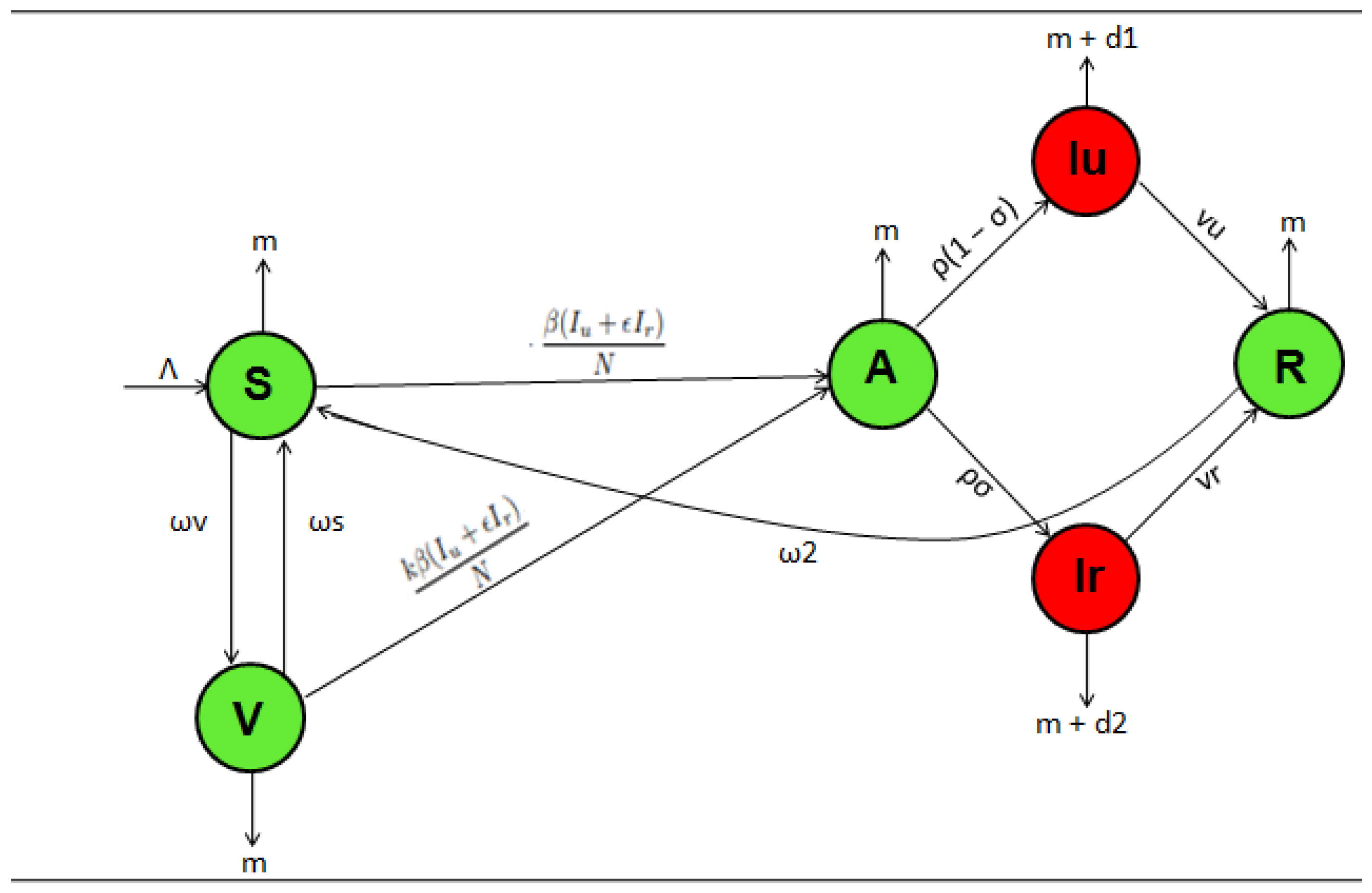
3. Mathematical Model Description

To formulate a mathematical model for the spread of coronavirus, considering the impact of vaccination, we divide the total population N ( t ) into six subclasses: susceptible S ( t ) , vaccinated V ( t ) , exposed A ( t ) , asymptomatic infected I u ( t ) , symptomatic infected I r ( t ) , and recovered R ( t ) . The susceptible class is generated by newborn babies at a rate of Λ . The number of susceptible individuals is decreased on the one hand by transmission to the exposed class at the rate ς ( I u + ϵ I r ) N , where ς is the effective contact rate with infected people and ϵ is the coefficient of symptomatic individuals, and on the other hand by vaccination at the rate ω V and natural mortality m, while it increases through the migration of both vaccinated and recovered people who lose immunity at the rates ω S and ω 2 , respectively. The group of exposed people grows by acquiring susceptible and vaccinated humans who have been in contact with infected individuals, while it decays by losing exposed people to the symptomatic and asymptomatic infected subclasses at the rates of ρ σ and ρ ( 1 σ ) , respectively. People displaying clear signs of illness are transmitted to the recovery group at a rate v u , while they die naturally or due to the coronavirus illness at the rates m and d 1 , respectively. Conversely, asymptomatic people become recovered at the rate v r and die due to the disease at the rate d 2 . Based on the above discussions and diagram (Figure 1):
Thus, the mathematical model is represented by the following system of differential equations:
d S d t = Λ + ω 2 R ς ( I u + ϵ I r ) N S ( ω V + m ) S + ω S V , d V d t = ω V S κ ς ( I u + ϵ I r ) N V ( ω S + m ) V , d A d t = ς ( I u + ϵ I r ) N S + ς κ ( I u + ϵ I r ) N V ( ρ + m ) A , d I u d t = ρ ( 1 σ ) A ( ν u + d 1 + m ) I u , d I r d t = ρ σ A ( ν r + d 2 + m ) I r , d R d t = ν u I u + ν r I r ( ω 2 + m ) R .
Furthermore, the initial conditions considered are as follows:
S ( 0 ) = S 0 0 , V ( 0 ) = V 0 0 , A ( 0 ) = A 0 0 , I u ( 0 ) = I u 0 0 , I r ( 0 ) = I r 0 0 , R ( 0 ) = R 0 0 .

Parameter Estimation Procedure

The method for estimating the model parameters is detailed in this section of the article. The conventional least-squares method is used for this objective. This method has been used in several recent publications and is employed to determine the optimal fit for a collection of data points by reducing the total of the offsets or residuals of points from the contoured curve [6,9,18]. Sources cited in [19] were used to determine the birth rate Λ and the natural mortality rate m. Figure 2 illustrates the curve of the model fit to the actual data points, while Table 1 enumerates the estimated and fitted parameters. The most crucial threshold parameter, the basic reproduction number, has an estimated numerical value of 1.20.

4. Mathematical Model Description by Fractal–Fractional Derivative

  0 C D t γ , θ S = Λ + ω 2 R ς ( I u + ϵ I r ) N S ( ω V + m ) S + ω S V ,   0 C D t γ , θ V = ω V S κ ς ( I u + ϵ I r ) N V ( m + ω S ) V ,   0 C D t γ , θ A = ς ( I u + ϵ I r ) N S + ς κ ( I u + ϵ I r ) N V ( ρ + m ) A ,   0 C D t γ , θ I u = ρ ( 1 σ ) A ( ν u + d 1 + m ) I u ,   0 C D t γ , θ I r = ρ σ A ( ν r + d 2 + m ) I r ,   0 C D t γ , θ R = ν u I u + ν r I r ( ω 2 + m ) R .
The following initial conditions apply:
S ( 0 ) = S 0 0 , V ( 0 ) = V 0 0 , A ( 0 ) = A 0 0 , I u ( 0 ) = I u 0 0 , I r ( 0 ) = I r 0 0 , R ( 0 ) = R 0 0 .
The system (6) and (7) can be rewritten in the following form:
  0 C D t γ , θ Y ( t ) = F ( Y ( t ) ) , Y ( 0 ) = Y 0 , 0 < t < T < ,
Here, the vector Y ( t ) = ( S ( t ) , V ( t ) , A ( t ) , I u ( t ) , I r ( t ) , R ( t ) ) T , and the operator F is defined as follows:
F ( Y ( t ) ) = F 1 ( Y ( t ) ) F 2 ( Y ( t ) ) F 3 ( Y ( t ) ) F 4 ( Y ( t ) ) F 5 ( Y ( t ) ) F 6 ( Y ( t ) ) = Λ + ω 2 R ς ( I u + ϵ I r ) N S ( ω V + m ) S + ω S V ω V S κ ς ( I u + ϵ I r ) N V ( m + ω S ) V ς ( I u + ϵ I r ) N S + κ ς ( I u + ϵ I r ) N V ( ρ + m ) A ρ ( 1 σ ) A ( m + ν u + d 1 ) I u ρ σ A ( ν r + m + d 2 ) I r ν u I u + ν r I r ( ω 2 + m ) R ,
The initial condition is
Y ( 0 ) = ( S ( 0 ) , V ( 0 ) , A ( 0 ) , I u ( 0 ) , I r ( 0 ) , R ( 0 ) ) .

4.1. Existence and Uniqueness Results

Next, we convert the system (6) into the following integral equation by using initial conditions (10) and Lemma 1:
Y ( t ) = Y ( 0 ) + θ Γ ( γ ) 0 t ( t s ) γ 1 s 1 θ × F ( Y ( s ) ) d s .
The existence and uniqueness of the solution of systems (6) and (7) are discussed in the generalized Banach space E = i = 1 6 C ( [ 0 , T ] , R ) endowed with the vector-valued norm . G defined by
. G : E R + 6 Y Y G = S V A I u I r R .
Theorem 2.
Assume the existence of a vector, each of whose components is positive, that satisfies
Υ = Υ 1 Υ 2 Υ 3 Υ 4 Υ 5 Υ 6 θ T γ + θ 1 Γ ( γ ) H ( γ , θ ) | Λ + ω 2 Υ 6 ς ( Υ 4 + ϵ Υ 5 ) N Υ 1 ( ω V + m ) Υ 1 + ω S Υ 2 | | ω V Υ 1 κ ς ( Υ 4 + ϵ Υ 5 ) N Υ 2 ( m + ω S ) Υ 2 | | ς ( Υ 4 + ϵ Υ 5 ) N Υ 1 + ς κ ( Υ 4 + ϵ Υ 5 ) N Υ 2 ( ρ + m ) Υ 3 | | ρ ( 1 σ ) Υ 3 ( ν u + d 1 + m ) Υ 4 | | ρ σ Υ 3 ( ν r + d 2 + m ) Υ 5 | | ν u Υ 4 + ν r Υ 5 ( ω 2 + m ) Υ 6 | ,
In addition, if the matrix θ T γ + θ 1 Γ ( γ ) H ( γ , θ ) converges to O 6 , where
= ς ( Υ 4 + ϵ Υ 5 ) N + ω V + m ω S 0 ϵ ς Υ 1 N ς Υ 1 N ω 2 ω V κ ς ( Υ 4 + ϵ Υ 5 ) N + m + ω S 0 κ ς Υ 2 N ϵ κ ς Υ 2 N 0 ς ( Υ 4 + ϵ Υ 5 ) N κ ς ( Υ 4 + ϵ Υ 5 ) N ρ + m ( ς Υ 1 + κ ς Υ 2 ) N ϵ ( ς Υ 1 + κ ς Υ 2 ) N 0 0 0 ρ ( 1 σ ) ( ν r + d 2 + m ) 0 0 0 0 ρ 0 ( ν r + d 2 + m ) 0 0 0 0 ν u ν r ( ω 2 + m ) ,
and given that H ( γ , θ ) represents the beta function for γ and θ, the system outlined in (6) and (7) possesses a unique solution within the specified space 1 6 C ( [ 0 , T ] ) , and the solution holds for all t > 0 in B ¯ ( Y 0 , Υ ) . Here, B ¯ ( Y 0 , Υ ) is the closed ball in the generalized Banach space i = 1 6 C ( [ 0 , T ] , R ) .
Proof. 
It is clear that Y is a solution to the systems (6) and (7) if and only if it satisfies the following equation:
Y ( t ) = M ( Y ( t ) ) ,
where M is the operator defined by M : i = 1 6 C ( [ 0 , T ] , R ) : i = 1 6 C ( [ 0 , T ] , R ) ,
M ( ( t ) ) = Y ( 0 ) + θ Γ ( γ ) 0 t ( t s ) γ 1 s 1 θ × F ( ( s ) ) d s .
We begin by proving that the operator defined above satisfies the following inequality:
M ( ) Y ( 0 ) G Υ R 6 . for any B ¯ ( Y 0 , Υ ) .
To this end, let B ¯ ( Y 0 , Υ ) , and we have
M ( ) Y ( 0 ) G = θ Γ ( γ ) 0 t ( t s ) γ 1 s 1 θ × F ( ( s ) ) d s G θ Γ ( γ ) 0 t ( t s ) γ 1 s 1 θ × F ( ) G d s θ Γ ( γ ) 0 t ( t s ) γ 1 s 1 θ L F θ T γ + θ 1 Γ ( γ ) H ( γ , θ ) L F θ T γ + θ 1 Γ ( γ ) H ( γ , θ ) L F
where
L F = sup B ¯ ( Y 0 , Υ ) F ( ) G | Λ + ω 2 Υ 6 ς ( Υ 4 + ϵ Υ 5 ) N Υ 1 ( ω V + m ) Υ 1 + ω S Υ 2 | | ω V Υ 1 κ ς ( Υ 4 + ϵ Υ 5 ) N Υ 2 ( m + ω S ) Υ 2 | | ς ( Υ 4 + ϵ Υ 5 ) N Υ 1 + ς κ ( Υ 4 + ϵ Υ 5 ) N Υ 2 ( ρ + m ) Υ 3 | | ρ ( 1 σ ) Υ 3 ( ν u + d 1 + m ) Υ 4 | | ρ σ Υ 3 ( ν r + d 2 + m ) Υ 5 | | ν u Υ 4 + ν r Υ 5 ( ω 2 + m ) Υ 6 | .
Then, the operator M maps B ¯ ( Y 0 , Υ ) onto itself. Further, let Y = ( S , V , A , I u , I r , R ) , Y ¯ = ( S ¯ , V ¯ , A ¯ , I u ¯ , I r ¯ , R ¯ ) B ¯ ( Y 0 , Υ ) , and when t falls within the interval [ 0 , T ] , we observe
F 1 ( Y ( t ) ) F 1 ( Y ¯ ( t ) ) = ω 2 ( R R ¯ ) ς ( I u + ϵ I r ) N S ς ( I u ¯ + ϵ I r ¯ ) N S ¯ ( ω V + m ) ( S S ¯ ) + ω S ( V V ¯ ) .
Then,
| F 1 ( Y ( t ) ) F 1 ( Y ¯ ( t ) ) | ω 2 | R R ¯ | + ς N | ( I u + ϵ I r ) S ( I u ¯ + ϵ I r ¯ ) S ¯ | + ( ω V + m ) | S S ¯ | + ω S | V V ¯ | ω 2 | R R ¯ | + ς N | I u S I u ¯ S ¯ | + ϵ ς N | I r S I r ¯ S ¯ | + ( ω V + m ω S ) | S S ¯ | .
Also, we have for all 1 , 2 , υ 1 , υ 2 R
| 1 υ 1 2 υ 2 | = 1 2 [ ( 1 2 ) ( υ 1 + υ 2 ) + ( 1 + 2 ) ( υ 1 υ 2 ) ] ,
Then,
| F 1 ( Y ( t ) ) F 1 ( Y ¯ ( t ) ) | ω 2 | R R ¯ |   +   ς 2 N | ( I u I u ¯ ) ( S   +   S ¯ )   +   ( I u   +   I u ¯ ) ( S S ¯ ) | +   ϵ ς 2 N | ( I r I r ¯ ) ( S   +   S ¯ )   +   ( I r   +   I r ¯ ) ( S S ¯ ) |   +   ( ω V   +   m ) | S S ¯ | +   ω S | V V ¯ | ω 2 | R R ¯ |   +   ς Υ 1 N | I u I u ¯ |   +   ς Υ 5 N | S S ¯ | +   ϵ ς Υ 1 N | I r I r ¯ |   +   ϵ ς Υ 4 N | S S ¯ |   +   ( ω V   +   m ) | S S ¯ |   +   ω S | V V ¯ | ω 2 | R R ¯ |   +   ς Υ 1 N | I u I u ¯ |   +   ϵ ς Υ 1 N | I r I r ¯ | +   ς Υ 5   +   ϵ ς Υ 4 N   +   ω V   +   m | S S ¯ |   +   ω S | V V ¯ | .
By determining the supremum across t, we derive
F 1 ( Y ) F 1 ( Y ¯ ) ω 2 R R ¯   +   ς Υ 1 N I u I u ¯   +   ϵ ς Υ 1 N I r I r ¯ +   ς ( Υ 5   +   ϵ Υ 4 ) N   +   ω V   +   m S S ¯   +   ω S V V ¯ .
In the same manner, we have
| F 2 ( Y ( t ) ) F 2 ( Y ¯ ( t ) ) | ω V | S S ¯ |   +   | κ ς ( I u   +   ϵ I r ) N V κ ς ( I u ¯   +   ϵ I r ¯ ) N V ¯ | +   ( m   +   ω S ) | V V ¯ | ω V | S S ¯ |   +   κ ς Υ 2 N | I u I u ¯ |   +   ϵ κ ς Υ 2 N | I r I r ¯ | +   κ ς Υ 5   +   κ ς ϵ Υ 4 N   +   m   +   ω S | V V ¯ | ,
Hence,
F 2 ( Y ) F 2 ( Y ¯ ) ω V S S ¯   +   κ ς Υ 2 N I u I u ¯   +   ϵ κ ς Υ 2 N I r I r ¯ +   κ ς ( Υ 5   +   ϵ Υ 4 ) N   +   m   +   ω S V V ¯ ,
| F 3 ( Y ( t ) ) F 3 ( Y ¯ ( t ) ) | ( ρ   +   m ) | A A ¯ |   +   | ς ( I u   +   ϵ I r ) N S ς ( I u ¯   +   ϵ I r ¯ ) N S ¯ | +   | κ ς ( I u   +   ϵ I r ) N V κ ς ( I u ¯   +   ϵ I r ¯ ) N V ¯ | ( ρ   +   m ) | A A ¯ |   +   ς Υ 1   +   κ ς Υ 2 N | I u I u ¯ | +   ϵ ( ς Υ 1   +   κ ς Υ 2 ) N | I r I r ¯ | +   ς ( Υ 5   +   ϵ Υ 4 ) N | S S ¯ | +   κ ς ( Υ 5   +   ϵ Υ 4 ) N | V V ¯ | ,
Then,
F 3 ( Y ) F 3 ( Y ¯ ) ( ρ + m ) A A ¯ + ς Υ 1 + κ ς Υ 2 N I u I u ¯ +   ϵ ( ς Υ 1 + κ ς Υ 2 ) N I r I r ¯ + ς ( Υ 5 + ϵ Υ 4 ) N S S ¯ + κ ς ( Υ 5 + ϵ Υ 4 ) N V V ¯ .
By the linearity of F 4 , F 5 , F 6 we can directly find
F 4 ( Y ) F 4 ( Y ¯ ) ρ ( 1 σ ) A A ¯ + ( ν u + d 1 + m ) I u I ¯ u ,
F 5 ( Y ) F 5 ( Y ¯ ) ρ σ A A ¯ + ( ν r + d 2 + m ) I r I ¯ r ,
F 6 ( Y ) F 6 ( Y ¯ ) ν u I u I ¯ u + ν r I r I ¯ r + ( ω 2 + m ) R R ¯ .
By rewriting Equations (15)–(20) in matrix form, we find
F ( Y ) F ( Y ¯ ) G = F 1 ( Y ) F 1 ( Y ¯ ) F 2 ( Y ) F 2 ( Y ¯ ) F 3 ( Y ) F 3 ( Y ¯ ) F 4 ( Y ) F 4 ( Y ¯ ) F 5 ( Y ) F 5 ( Y ¯ ) F 6 ( Y ) F 6 ( Y ¯ ) S S ¯ V V ¯ A A ¯ I u I ¯ u I r I ¯ r R R ¯ ,
where ℧ is defined in (2). Then, F is a G-Lipschitz operator. By using this fact, we conclude that for any Y , Y ¯ B ¯ ( Y 0 , Υ ) :
M ( Y ) M ( Y ¯ ) G θ Γ ( γ ) 0 t ( t s ) γ 1 s 1 θ × F ( Y ) F ( Y ¯ ) G d s θ Γ ( γ ) 0 t ( t s ) γ 1 s 1 θ Y Y ¯ G θ T γ + θ 1 Γ ( γ ) H ( γ , θ ) Y Y ¯ G .
Since the matrix θ T γ + θ 1 Γ ( γ ) H ( γ , θ ) converges to zero, the operator M is a G-contraction; hence, by applying the Perov fixed point theorem 1, the systems (6) and (7) have a unique solution. □

4.2. Stability Analysis of the Fractal–Fractional COVID-19 Model in the Ulam–Hyers Context

In this subsection, we aim to establish the Ulam–Hyers stability for our suggested model, drawing on definitions from [20].
Definition 7.
Let ( X , d G ) be a generalized metric space and F : X X be an operator. Then, the fixed point equation
X = F ( X )
is said to be generalized Ulam–Hyers stable (GUHS) if there exists an increasing function ψ : R + m R + m , continuous in 0 R m with ψ ( 0 ) = 0 , such that, for any ε : = ε 1 , , ε m with ε i > 0 for i { 1 , , m } and any solution Y * X of the inequalities
d G ( Y * , F ( Y * ) ) ε ,
there exists a solution X * of (21) such that
d G X * , Y * ψ ( ε ) .
Consider a small perturbation Φ : = ( Φ 1 , Φ 2 , Φ 3 , Φ 4 , Φ 5 , Φ 6 ) C ( [ 0 , T ] ) 6 such that Φ ( 0 R 3 ) = 0 R 3 . Let the following hold:
  • For each i = 1 , , 3 , it holds that | Φ i ( t ) | does not exceed ε i , with ε i being a positive constant.
  • The absolute value of Φ i ( t ) is bounded by ε i , where ε i > 0 for each i = 1 , , 3 .
  • | Φ i ( t ) | ε i , for ε i > 0 i = 1 , , 3 .
  •   0 C D t γ , θ S = Λ + ω 2 R ς ( I u + ϵ I r ) N S ( ω V + m ) S + ω S V + Φ 1 ,   0 C D t γ , θ V = ω V S κ ς ( I u + ϵ I r ) N V ( m + ω S ) V + Φ 2 ,   0 C D t γ , θ A = ς ( I u + ϵ I r ) N S + κ ς ( I u + ϵ I r ) N V ( ρ + m ) A + Φ 3 ,   0 C D t γ , θ I u = ρ ( 1 σ ) A ( ν u + d 1 + m ) I u + Φ 4 ,   0 C D t γ , θ I r = ρ σ A ( ν r + d 2 + m ) I r + Φ 5 ,   0 C D t γ , θ R = ν u I u + ν r I r ( ω 2 + m ) R + Φ 6 .
Lemma 2.
The solution of the perturbed model
  0 C D t γ S = θ t θ 1 Λ + ω 2 R ς ( I u + ϵ I r ) N S ( ω V + m ) S + ω S V + Φ 1 ,   0 C D t γ V = θ t θ 1 ω V S κ ς ( I u + ϵ I r ) N V ( m + ω S ) V + Φ 2 ,   0 C D t γ A = θ t θ 1 ς ( I u + ϵ I r ) N S + κ ς ( I u + ϵ I r ) N V ( ρ + m ) A + Φ 3 ,   0 C D t γ I u = θ t θ 1 ρ ( 1 σ ) A ( ν u + d 1 + m ) I u + Φ 4 ,   0 C D t γ I r = θ t θ 1 ρ σ A ( ν r + d 2 + m ) I r + Φ 5 ,   0 C D t γ R = θ t θ 1 ν u I u + ν r I r ( ω 2 + m ) R + Φ 6 .
fulfills the relation given below:
S ( t ) S ( 0 ) + θ Γ ( γ ) 0 t s θ 1 ( t s ) γ 1 F 1 ( X ) ( s ) d s V ( t ) V ( 0 ) + θ Γ ( γ ) 0 t s θ 1 ( t s ) γ 1 F 2 ( X ) ( t ) d s A ( t ) A ( 0 ) + θ Γ ( γ ) 0 t s θ 1 ( t s ) γ 1 F 3 ( X ) ( s ) d s I u ( t ) I u ( 0 ) + θ Γ ( γ ) 0 t s θ 1 ( t s ) γ 1 F 4 ( X ) ( s ) d s I r ( t ) I r ( 0 ) + θ Γ ( γ ) 0 t s θ 1 ( t s ) γ 1 F 5 ( X ) ( s ) d s R ( t ) R ( 0 ) + θ Γ ( γ ) 0 t s θ 1 ( t s ) γ 1 F 6 ( X ) ( s ) d s G θ T γ + θ 1 Γ ( γ ) H ( γ , θ ) ε 1 ε 2 ε 3 ε 4 ε 5 ε 6 .
Proof. 
The resolution of (23) is expressed as
S ( t ) = S ( 0 ) + θ Γ ( γ ) 0 t s θ 1 ( t s ) γ 1 F 1 ( X ) ( s ) + Φ 1 d s , V ( t ) = V ( 0 ) + θ Γ ( γ ) 0 t s θ 1 ( t s ) γ 1 F 2 ( X ) ( s ) + Φ 2 d s , A ( t ) = A ( 0 ) + θ Γ ( γ ) 0 t s θ 1 ( t s ) γ 1 F 3 ( X ) ( s ) + Φ 3 d s . I u ( t ) = I u ( 0 ) + θ Γ ( γ ) 0 t s θ 1 ( t s ) γ 1 F 4 ( X ) ( s ) + Φ 4 d s , I r ( t ) = I r ( 0 ) + θ Γ ( γ ) 0 t s θ 1 ( t s ) γ 1 F 5 ( X ) ( s ) + Φ 5 d s , R ( t ) = R ( 0 ) + θ Γ ( γ ) 0 t s θ 1 ( t s ) γ 1 F 6 ( X ) ( s ) + Φ 6 d s .
Then, we have
sup t [ 0 T ] | S ( t ) S 0 + θ Γ ( γ ) 0 t s θ 1 ( t s ) γ 1 F 1 ( X ) ( s ) d s | = sup t [ 0 T ] | S 0 + θ Γ ( γ ) × 0 t ( t s ) γ 1 s 1 θ F 1 ( X ) ( s ) + Φ 1 ( s ) d s S 0 + θ Γ ( γ ) 0 t s θ 1 ( t s ) γ 1 F 1 ( X ) ( s ) d s | = sup t [ 0 T ] | θ Γ ( γ ) 0 t ( t s ) γ 1 s 1 θ Φ 1 ( s ) | θ T γ + θ 1 Γ ( γ ) H ( γ , θ ) ε 1 .
Repeating the same procedure as the rest of the equations of system (23), we have
sup t [ 0 T ] | V ( t ) V 0 + θ Γ ( γ ) 0 t s θ 1 ( t s ) γ 1 F 2 ( X ) ( s ) d s | θ T γ + θ 1 Γ ( γ ) H ( γ , θ ) ε 2 .
sup t [ 0 T ] | A ( t ) A 0 + θ Γ ( γ ) 0 t s θ 1 ( t s ) γ 1 F 3 ( X ) ( s ) d s | θ T γ + θ 1 Γ ( γ ) H ( γ , θ ) ε 3 .
sup t [ 0 T ] | I u ( t ) I u 0 + θ Γ ( γ ) 0 t s θ 1 ( t s ) γ 1 F 4 ( X ) ( s ) d s | θ T γ + θ 1 Γ ( γ ) H ( γ , θ ) ε 4 .
sup t [ 0 T ] | I r ( t ) I r 0 + θ Γ ( γ ) 0 t s θ 1 ( t s ) γ 1 F 5 ( X ) ( s ) d s | θ T γ + θ 1 Γ ( γ ) H ( γ , θ ) ε 5 .
sup t [ 0 T ] | R ( t ) R 0 + θ Γ ( γ ) 0 t s θ 1 ( t s ) γ 1 F 6 ( X ) ( s ) d s | θ T γ + θ 1 Γ ( γ ) H ( γ , θ ) ε 6 .
Hence, the proof is completed. □
Theorem 3.
If the matrix θ T γ + θ 1 Γ ( γ ) H ( γ , θ ) (2) converges to O 6 , then (6) is generalized Ulam–Hyers stable (GUHS).
Proof. 
Assuming X = ( S , V , A , I u , I r , R ) represents a possible resolution of the inequality (24), and X * = ( S * , V * , A * , I u * , I r * , R * ) is the distinct solution of (6), then
S S * = sup t [ 0 T ] S ( t ) S 0 * + θ Γ ( γ ) 0 t s θ 1 ( t s ) γ 1 F 1 ( X * ) ( s ) d s sup t [ 0 T ] S ( t ) S 0 + θ Γ ( γ ) 0 t s θ 1 ( t s ) γ 1 F 1 ( X ) ( s ) d s + sup t [ 0 T ] S 0 + θ Γ ( γ ) 0 t s θ 1 ( t s ) γ 1 F 1 ( X ) ( s ) d s S 0 * + θ Γ ( γ ) 0 t s θ 1 ( t s ) γ 1 F 1 ( X * ) ( s ) d s θ T γ + θ 1 Γ ( γ ) H ( γ , θ ) ε 1 + θ T γ + θ 1 Γ ( γ ) H ( γ , θ ) ( ω 2 R R * + ς Υ 1 N I u I u * + ϵ ς Υ 1 N I r I r * + ς ( Υ 4 + ϵ Υ 5 ) N + ω V + m S S * + ω S V V * ) .
In the same manner, we find
V V * θ T γ + θ 1 Γ ( γ ) H ( γ , θ ) ε 2 + θ T γ + θ 1 Γ ( γ ) H ( γ , θ ) ( ω V S S * + κ ς Υ 2 N I u I u * + ϵ κ ς Υ 2 N I r I r * + κ ς ( Υ 4 + ϵ Υ 5 ) N + m + ω S V V * ) ,
and
A A * θ T γ + θ 1 Γ ( γ ) H ( γ , θ ) ε 3 + θ T γ + θ 1 Γ ( γ ) H ( γ , θ ) ( ( ρ + m ) A A * + ς Υ 1 + κ ς Υ 2 N I u I u * + ϵ ( ς Υ 1 + κ ς Υ 2 ) N I r I r * + ς ( Υ 4 + ϵ Υ 5 ) N S S * + κ ς ( Υ 4 + ϵ Υ 5 ) N V V * ) ,
I u I u * θ T γ + θ 1 Γ ( γ ) H ( γ , θ ) ε 4 + θ T γ + θ 1 Γ ( γ ) H ( γ , θ ) ( ρ ( 1 σ ) A A + ( ν u + d 1 + m ) I u I u * ) ,
I r I r * θ T γ + θ 1 Γ ( γ ) H ( γ , θ ) ε 5 + θ T γ + θ 1 Γ ( γ ) H ( γ , θ ) ( ρ σ A A * + ( ν r + d 2 + m ) I r I r * ) ,
R R * θ T γ + θ 1 Γ ( γ ) H ( γ , θ ) ε 6 + θ T γ + θ 1 Γ ( γ ) H ( γ , θ ) ( ν u I u I u * + ν r I r I r * + ( ω 2 + m ) R R * ) ,
Consequently, one can write
X X * G θ T γ + θ 1 Γ ( γ ) H ( γ , θ ) ε 1 ε 2 ε 3 ε 4 ε 5 ε 6 + X X * G .
Considering the convergence of the matrix ℧ to zero, it then follows that
X X * G I 6 θ T γ + θ 1 Γ ( γ ) H ( γ , θ ) 1 θ T γ + θ 1 Γ ( γ ) H ( γ , θ ) ε 1 ε 2 ε 3 ε 4 ε 5 ε 6 .
Therefore, (6) exhibits GUHS. □

5. Numerical Scheme for the FF Model

In this section, we employ a two-step Newton polynomial approximation [21] to establish the numerical schemes for our fractal–fractional model describing coronavirus dynamics. We reorder the fractal–fractional problem as follows:
  0 C D t γ S ( t ) = θ t θ 1 F 1 ( t , S ( t ) , V ( t ) , A ( t ) , I u ( t ) , I r ( t ) , R ( t ) )   0 C D t γ V ( t ) = θ t θ 1 F 2 ( t , S ( t ) , V ( t ) , A ( t ) , I u ( t ) , I r ( t ) , R ( t ) )   0 C D t γ A ( t ) = θ t θ 1 F 3 ( t , S ( t ) , V ( t ) , A ( t ) , I u ( t ) , I r ( t ) , R ( t ) )   0 C D t γ I u ( t ) = θ t θ 1 F 4 ( t , S ( t ) , V ( t ) , A ( t ) , I u ( t ) , I r ( t ) , R ( t ) )   0 C D t γ I r ( t ) = θ t θ 1 F 5 ( t , S ( t ) , V ( t ) , A ( t ) , I u ( t ) , I r ( t ) , R ( t ) )   0 C D t γ R ( t ) = θ t θ 1 F 6 ( t , S ( t ) , V ( t ) , A ( t ) , I u ( t ) , I r ( t ) , R ( t ) ) .
At the point t n + 1 , we have the following:
S ( t n + 1 ) = S ( 0 ) + θ Γ ( γ ) 0 t n + 1 τ θ 1 ( t n + 1 τ ) γ 1 F 1 ( τ , S ( τ ) , V ( t ) , A ( τ ) , I u ( τ ) , I r ( τ ) , R ( τ ) ) d τ , V ( t n + 1 ) = V ( 0 ) + θ Γ ( γ ) 0 t n + 1 τ θ 1 ( t n + 1 τ ) γ 1 F 2 ( τ , S ( τ ) , V ( t ) , A ( τ ) , I u ( τ ) , I r ( τ ) , R ( τ ) ) d τ , A ( t n + 1 ) = A ( 0 ) + θ Γ ( γ ) 0 t n + 1 τ θ 1 ( t n + 1 τ ) γ 1 F 3 ( τ , S ( τ ) , V ( t ) , A ( τ ) , I u ( τ ) , I r ( τ ) , R ( τ ) ) d τ , I u ( t n + 1 ) = I u ( 0 ) + θ Γ ( γ ) 0 t n + 1 τ θ 1 ( t n + 1 τ ) γ 1 F 4 ( τ , S ( τ ) , V ( t ) , A ( τ ) , I u ( τ ) , I r ( τ ) , R ( τ ) ) d τ , I r ( t n + 1 ) = I r ( 0 ) + θ Γ ( γ ) 0 t n + 1 τ θ 1 ( t n + 1 τ ) γ 1 F 5 ( τ , S ( τ ) , V ( t ) , A ( τ ) , I u ( τ ) , I r ( τ ) , R ( τ ) ) d τ , R ( t n + 1 ) = R ( 0 ) + θ Γ ( γ ) 0 t n + 1 τ θ 1 ( t n + 1 τ ) γ 1 F 6 ( τ , S ( τ ) , V ( t ) , A ( τ ) , I u ( τ ) , I r ( τ ) , R ( τ ) ) d τ .
Thus, we can write
S ( t n + 1 ) = S ( 0 ) + θ Γ ( γ ) p = 2 n t p t p + 1 τ θ 1 ( t n + 1 τ ) γ 1 F 1 ( τ , S ( τ ) , V ( t ) , A ( τ ) , I u ( τ ) , I r ( τ ) , R ( τ ) ) d τ V ( t n + 1 ) = V ( 0 ) + θ Γ ( γ ) p = 2 n t p t p + 1 τ θ 1 ( t n + 1 τ ) γ 1 F 2 ( τ , S ( τ ) , V ( t ) , A ( τ ) , I u ( τ ) , I r ( τ ) , R ( τ ) ) d τ A ( t n + 1 ) = A ( 0 ) + θ Γ ( γ ) p = 2 n t p t p + 1 τ θ 1 ( t n + 1 τ ) γ 1 F 3 ( τ , S ( τ ) , V ( t ) , A ( τ ) , I u ( τ ) , I r ( τ ) , R ( τ ) ) d τ I u ( t n + 1 ) = I u ( 0 ) + θ Γ ( γ ) p = 2 n t p t p + 1 τ θ 1 ( t n + 1 τ ) γ 1 F 4 ( τ , S ( τ ) , V ( t ) , A ( τ ) , I u ( τ ) , I r ( τ ) , R ( τ ) ) d τ I r ( t n + 1 ) = I r ( 0 ) + θ Γ ( γ ) p = 2 n t p t p + 1 τ θ 1 ( t n + 1 τ ) γ 1 F 5 ( τ , S ( τ ) , V ( t ) , A ( τ ) , I u ( τ ) , I r ( τ ) , R ( τ ) ) d τ R ( t n + 1 ) = R ( 0 ) + θ Γ ( γ ) p = 2 n t p t p + 1 τ θ 1 ( t n + 1 τ ) γ 1 F 6 ( τ , S ( τ ) , V ( t ) , A ( τ ) , I u ( τ ) , I r ( τ ) , R ( τ ) ) d τ .
Using the two steps of the Newton polynomial, we obtain
S ( t n + 1 ) = S ( 0 ) + θ Γ ( γ ) m = 2 n t m t m + 1 F 1 ( t m 2 , S m 2 , V m 2 , A m 2 , I u m 2 , I r m 2 , R m 2 ) + [ F 1 ( t m 1 , S m 1 , V m 1 , A m 1 , I u m 1 , I r m 1 , R m 1 ) h F 1 ( t m 2 , S m 2 , V m 2 , A m 2 , I u m 2 , I r m 2 , R m 2 ) h ] ( τ t m 2 ) + [ F 1 ( t m , S m , V m , A m , I u m , I r m , R m ) 2 h 2 2 F 1 ( t m 1 , S m 1 , V m 1 , A m 1 , I u m 1 , I r m 1 , R m 1 ) 2 h 2 + F 1 ( t m 2 , S m 2 , V m 2 , A m 2 , I u m 2 , I r m 2 , R m 2 ) 2 h 2 ] ( τ t m 2 ) ( τ t m 1 ) ( t n + 1 τ ) γ 1 d τ , V ( t n + 1 ) = V ( 0 ) + θ Γ ( γ ) m = 2 n t m t m + 1 F 2 ( t m 2 , S m 2 , V m 2 , A m 2 , I u m 2 , I r m 2 , R m 2 ) + [ F 2 ( t m 1 , S m 1 , V m 1 , A m 1 , I u m 1 , I r m 1 , R m 1 ) h F 2 ( t m 2 , S m 2 , V m 2 , A m 2 , I u m 2 , I r m 2 , R m 2 ) h ] ( τ t m 2 ) + [ F 2 ( t m , S m , V m , A m , I u m , I r m , R m ) 2 h 2 2 F 2 ( t m 1 , S m 1 , V m 1 , A m 1 , I u m 1 , I r m 1 , R m 1 ) 2 h 2 + F 1 ( t m 2 , S m 2 , V m 2 , A m 2 , I u m 2 , I r m 2 , R m 2 ) 2 h 2 ] ( τ t m 2 ) ( τ t m 1 ) ( t n + 1 τ ) γ 1 d τ , A ( t n + 1 ) = A ( 0 ) + θ Γ ( γ ) m = 2 n t m t m + 1 F 3 ( t m 2 , S m 2 , V m 2 , A m 2 , I u m 2 , I r m 2 , R m 2 ) + [ F 3 ( t m 1 , S m 1 , V m 1 , A m 1 , I u m 1 , I r m 1 , R m 1 ) h F 3 ( t m 2 , S m 2 , V m 2 , A m 2 , I u m 2 , I r m 2 , R m 2 ) h ] ( τ t m 2 ) + [ F 3 ( t m , S m , V m , A m , I u m , I r m , R m ) 2 h 2 2 F 3 ( t m 1 , S m 1 , V m 1 , A m 1 , I u m 1 , I r m 1 , R m 1 ) 2 h 2 + F 3 ( t m 2 , S m 2 , V m 2 , A m 2 , I u m 2 , I r m 2 , R m 2 ) 2 h 2 ] ( τ t m 2 ) ( τ t m 1 ) ( t n + 1 τ ) γ 1 d τ ,
I u ( t n + 1 ) = I u ( 0 ) + θ Γ ( γ ) m = 2 n t m t m + 1 F 4 ( t m 2 , S m 2 , V m 2 , A m 2 , I u m 2 , I r m 2 , R m 2 ) + [ F 4 ( t m 1 , S m 1 , V m 1 , A m 1 , I u m 1 , I r m 1 , R m 1 ) h F 4 ( t m 2 , S m 2 , V m 2 , A m 2 , I u m 2 , I r m 2 , R m 2 ) h ] ( τ t m 2 ) + [ F 4 ( t m , S m , V m , A m , I u m , I r m , R m ) 2 h 2 2 F 4 ( t m 1 , S m 1 , V m 1 , A m 1 , I u m 1 , I r m 1 , R m 1 ) 2 h 2 + F 4 ( t m 2 , S m 2 , V m 2 , A m 2 , I u m 2 , I r m 2 , R m 2 ) 2 h 2 ] ( τ t m 2 ) ( τ t m 1 ) ( t n + 1 τ ) γ 1 d τ , I r ( t n + 1 ) = I r ( 0 ) + θ Γ ( γ ) m = 2 n t m t m + 1 F 5 ( t m 2 , S m 2 , V m 2 , A m 2 , I u m 2 , I r m 2 , R m 2 ) + [ F 5 ( t m 1 , S m 1 , V m 1 , A m 1 , I u m 1 , I r m 1 , R m 1 ) h F 5 ( t m 2 , S m 2 , V m 2 , A m 2 , I u m 2 , I r m 2 , R m 2 ) h ] ( τ t m 2 ) + [ F 5 ( t m , S m , V m , A m , I u m , I r m , R m ) 2 h 2 2 F 5 ( t m 1 , S m 1 , V m 1 , A m 1 , I u m 1 , I r m 1 , R m 1 ) 2 h 2 + F 5 ( t m 2 , S m 2 , V m 2 , A m 2 , I u m 2 , I r m 2 , R m 2 ) 2 h 2 ] ( τ t m 2 ) ( τ t m 1 ) ( t n + 1 τ ) γ 1 d τ , R ( t n + 1 ) = R ( 0 ) + θ Γ ( γ ) m = 2 n t m t m + 1 F 6 ( t m 2 , S m 2 , V m 2 , A m 2 , I u m 2 , I r m 2 , R m 2 ) + [ F 6 ( t m 1 , S m 1 , V m 1 , A m 1 , I u m 1 , I r m 1 , R m 1 ) h F 6 ( t m 2 , S m 2 , V m 2 , A m 2 , I u m 2 , I r m 2 , R m 2 ) h ] ( τ t m 2 ) + [ F 6 ( t m , S m , V m , A m , I u m , I r m , R m ) 2 h 2 2 F 6 ( t m 1 , S m 1 , V m 1 , A m 1 , I u m 1 , I r m 1 , R m 1 ) 2 h 2 + F 6 ( t m 2 , S m 2 , V m 2 , A m 2 , I u m 2 , I r m 2 , R m 2 ) 2 h 2 ] ( τ t m 2 ) ( τ t m 1 ) ( t n + 1 τ ) γ 1 d τ .
After some calculation, we obtain the numerical scheme for Model (6) of the coronavirus epidemic as follows:
S ( t n + 1 ) = S 0 + h γ Γ ( γ + 1 ) m = 2 n θ t m 2 θ 1 F 1 ( t m 2 , S m 2 , V m 2 , A m 2 , I u m 2 , I r m 2 , R m 2 ) ( n m + 1 ) γ ( n m ) γ +   h γ Γ ( γ + 2 ) m = 2 n [ θ t m 1 θ 1 F 1 ( t m 1 , S m 1 , V m 1 , A m 1 , I u m 1 , I r m 1 , R m 1 ) θ t m 2 θ 1 F 1 ( t m 2 , S m 2 , V m 2 , A m 2 , I u m 2 , I r m 2 , R m 2 ) ] ( n m + 1 ) γ ( n m + 3 + 2 γ ) ( n m ) γ ( n m + 3 + 3 γ ) +   h γ 2 Γ ( γ + 3 ) m = 2 n [ θ t m θ 1 F 1 ( t m , S m , V m , A m , I u m , I r m , R m )   2 θ t m 1 θ 1 F 1 ( t m 1 , S m 1 , V m 1 , A m 1 , I u m 1 , I r m 1 , R m 1 ) +   θ t m 2 θ 1 F 1 ( t m 2 , S m 2 , V m 2 , A m 2 , I u m 2 , I r m 2 , R m 2 ) ] ×   [ ( n m + 1 ) γ [ 2 ( n m ) 2 + ( 3 γ + 10 ) ( n m ) + 2 γ 2 + 9 γ + 12 ]   ( n m ) γ [ 2 ( n m ) 2 + ( 5 γ + 10 ) ( n m ) + 6 γ 2 + 18 γ + 12 ] ] ,
V ( t n + 1 ) = V 0 + h γ Γ ( γ + 1 ) m = 2 n θ t m 2 θ 1 F 2 ( t m 2 , S m 2 , V m 2 , A m 2 , I u m 2 , I r m 2 , R m 2 ) ( n m + 1 ) γ ( n m ) γ +   h γ Γ ( γ + 2 ) m = 2 n [ θ t m 1 θ 1 F 2 ( t m 1 , S m 1 , V m 1 , A m 1 , I u m 1 , I r m 1 , R m 1 ) θ t m 2 θ 1 F 2 ( t m 2 , S m 2 , V m 2 , A m 2 , I u m 2 , I r m 2 , R m 2 ) ] ( n m + 1 ) γ ( n m + 3 + 2 γ ) ( n m ) γ ( n m + 3 + 3 γ ) +   h γ 2 Γ ( γ + 3 ) m = 2 n [ θ t m θ 1 F 2 ( t m , S m , V m , A m , I u m , I r m , R m )   2 θ t m 1 θ 1 F 2 ( t m 1 , S m 1 , V m 1 , A m 1 , I u m 1 , I r m 1 , R m 1 ) +   θ t m 2 θ 1 F 2 ( t m 2 , S m 2 , V m 2 , A m 2 , I u m 2 , I r m 2 , R m 2 ) ] ×   [ ( n m + 1 ) γ [ 2 ( n m ) 2 + ( 3 γ + 10 ) ( n m ) + 2 γ 2 + 9 γ + 12 ]   ( n m ) γ [ 2 ( n m ) 2 + ( 5 γ + 10 ) ( n m ) + 6 γ 2 + 18 γ + 12 ] ] , ,
A ( t n + 1 ) = A 0 + h γ Γ ( γ + 1 ) m = 2 n θ t m 2 θ 1 F 3 ( t m 2 , S m 2 , V m 2 , A m 2 , I u m 2 , I r m 2 , R m 2 ) ( n m + 1 ) γ ( n m ) γ +   h γ Γ ( γ + 2 ) m = 2 n [ θ t m 1 θ 1 F 3 ( t m 1 , S m 1 , V m 1 , A m 1 , I u m 1 , I r m 1 , R m 1 ) θ t m 2 θ 1 F 3 ( t m 2 , S m 2 , V m 2 , A m 2 , I u m 2 , I r m 2 , R m 2 ) ] ( n m + 1 ) γ ( n m + 3 + 2 γ ) ( n m ) γ ( n m + 3 + 3 γ ) +   h γ 2 Γ ( γ + 3 ) m = 2 n [ θ t m θ 1 F 3 ( t m , S m , V m , A m , I u m , I r m , R m )   2 θ t m 1 θ 1 F 3 ( t m 1 , S m 1 , V m 1 , A m 1 , I u m 1 , I r m 1 , R m 1 ) +   θ t m 2 θ 1 F 3 ( t m 2 , S m 2 , V m 2 , A m 2 , I u m 2 , I r m 2 , R m 2 ) ] ×   [ ( n m + 1 ) γ [ 2 ( n m ) 2 + ( 3 γ + 10 ) ( n m ) + 2 γ 2 + 9 γ + 12 ]   ( n m ) γ [ 2 ( n m ) 2 + ( 5 γ + 10 ) ( n m ) + 6 γ 2 + 18 γ + 12 ] ] , ,
I u ( t n + 1 ) = I u 0 + h γ Γ ( γ + 1 ) m = 2 n θ t m 2 θ 1 F 4 ( t m 2 , S m 2 , V m 2 , A m 2 , I u m 2 , I r m 2 , R m 2 ) ( n m + 1 ) γ ( n m ) γ +   h γ Γ ( γ + 2 ) m = 2 n [ θ t m 1 θ 1 F 4 ( t m 1 , S m 1 , V m 1 , A m 1 , I u m 1 , I r m 1 , R m 1 ) θ t m 2 θ 1 F 4 ( t m 2 , S m 2 , V m 2 , A m 2 , I u m 2 , I r m 2 , R m 2 ) ] ( n m + 1 ) γ ( n m + 3 + 2 γ ) ( n m ) γ ( n m + 3 + 3 γ ) +   h γ 2 Γ ( γ + 3 ) m = 2 n [ θ t m θ 1 F 4 ( t m , S m , V m , A m , I u m , I r m , R m )   2 θ t m 1 θ 1 F 4 ( t m 1 , S m 1 , V m 1 , A m 1 , I u m 1 , I r m 1 , R m 1 ) +   θ t m 2 θ 1 F 4 ( t m 2 , S m 2 , V m 2 , A m 2 , I u m 2 , I r m 2 , R m 2 ) ] ×   [ ( n m + 1 ) γ [ 2 ( n m ) 2 + ( 3 γ + 10 ) ( n m ) + 2 γ 2 + 9 γ + 12 ]   ( n m ) γ [ 2 ( n m ) 2 + ( 5 γ + 10 ) ( n m ) + 6 γ 2 + 18 γ + 12 ] ] , ,
I r ( t n + 1 ) = I r 0 + h γ Γ ( γ + 1 ) m = 2 n θ t m 2 θ 1 F 5 ( t m 2 , S m 2 , V m 2 , A m 2 , I u m 2 , I r m 2 , R m 2 ) ( n m + 1 ) γ ( n m ) γ +   h γ Γ ( γ + 2 ) m = 2 n [ θ t m 1 θ 1 F 5 ( t m 1 , S m 1 , V m 1 , A m 1 , I u m 1 , I r m 1 , R m 1 ) θ t m 2 θ 1 F 5 ( t m 2 , S m 2 , V m 2 , A m 2 , I u m 2 , I r m 2 , R m 2 ) ] ( n m + 1 ) γ ( n m + 3 + 2 γ ) ( n m ) γ ( n m + 3 + 3 γ ) +   h γ 2 Γ ( γ + 3 ) m = 2 n [ θ t m θ 1 F 5 ( t m , S m , V m , A m , I u m , I r m , R m )   2 θ t m 1 θ 1 F 5 ( t m 1 , S m 1 , V m 1 , A m 1 , I u m 1 , I r m 1 , R m 1 ) +   θ t m 2 θ 1 F 5 ( t m 2 , S m 2 , V m 2 , A m 2 , I u m 2 , I r m 2 , R m 2 ) ] ×   [ ( n m + 1 ) γ [ 2 ( n m ) 2 + ( 3 γ + 10 ) ( n m ) + 2 γ 2 + 9 γ + 12 ]   ( n m ) γ [ 2 ( n m ) 2 + ( 5 γ + 10 ) ( n m ) + 6 γ 2 + 18 γ + 12 ] ] ,
R ( t n + 1 ) = R 0 + h γ Γ ( γ + 1 ) m = 2 n θ t m 2 θ 1 F 6 ( t m 2 , S m 2 , V m 2 , A m 2 , I u m 2 , I r m 2 , R m 2 ) ( n m + 1 ) γ ( n m ) γ +   h γ Γ ( γ + 2 ) m = 2 n [ θ t m 1 θ 1 F 6 ( t m 1 , S m 1 , V m 1 , A m 1 , I u m 1 , I r m 1 , R m 1 ) θ t m 2 θ 1 F 6 ( t m 2 , S m 2 , V m 2 , A m 2 , I u m 2 , I r m 2 , R m 2 ) ] ( n m + 1 ) γ ( n m + 3 + 2 γ ) ( n m ) γ ( n m + 3 + 3 γ ) +   h γ 2 Γ ( γ + 3 ) m = 2 n [ θ t m θ 1 F 6 ( t m , S m , V m , A m , I u m , I r m , R m )   2 θ t m 1 θ 1 F 6 ( t m 1 , S m 1 , V m 1 , A m 1 , I u m 1 , I r m 1 , R m 1 ) +   θ t m 2 θ 1 F 6 ( t m 2 , S m 2 , V m 2 , A m 2 , I u m 2 , I r m 2 , R m 2 ) ] ×   [ ( n m + 1 ) γ [ 2 ( n m ) 2 + ( 3 γ + 10 ) ( n m ) + 2 γ 2 + 9 γ + 12 ]   ( n m ) γ [ 2 ( n m ) 2 + ( 5 γ + 10 ) ( n m ) + 6 γ 2 + 18 γ + 12 ] ] . .

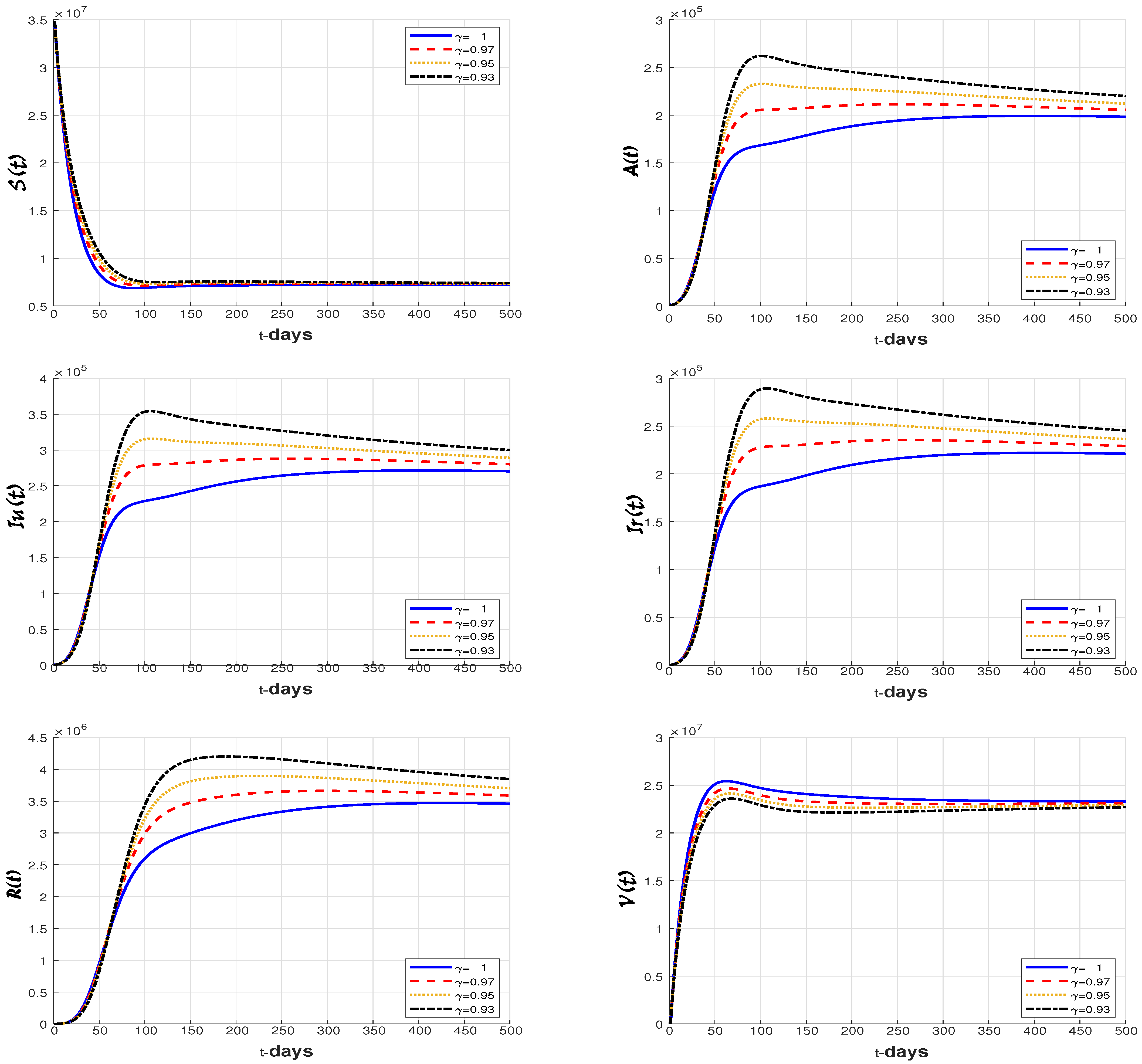
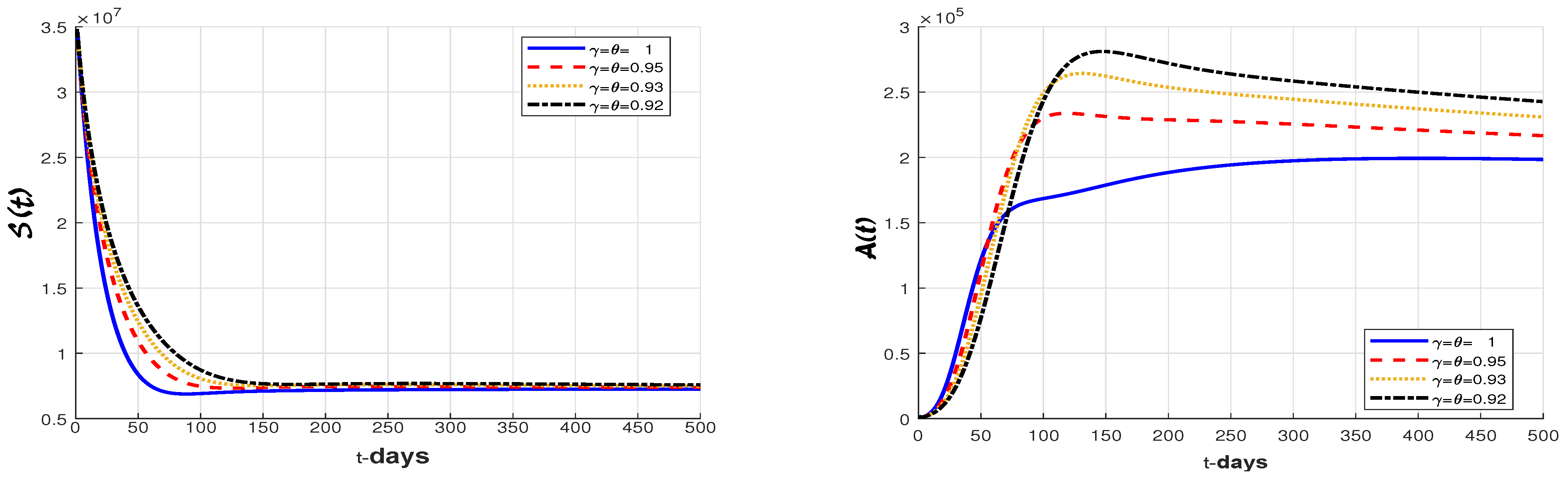
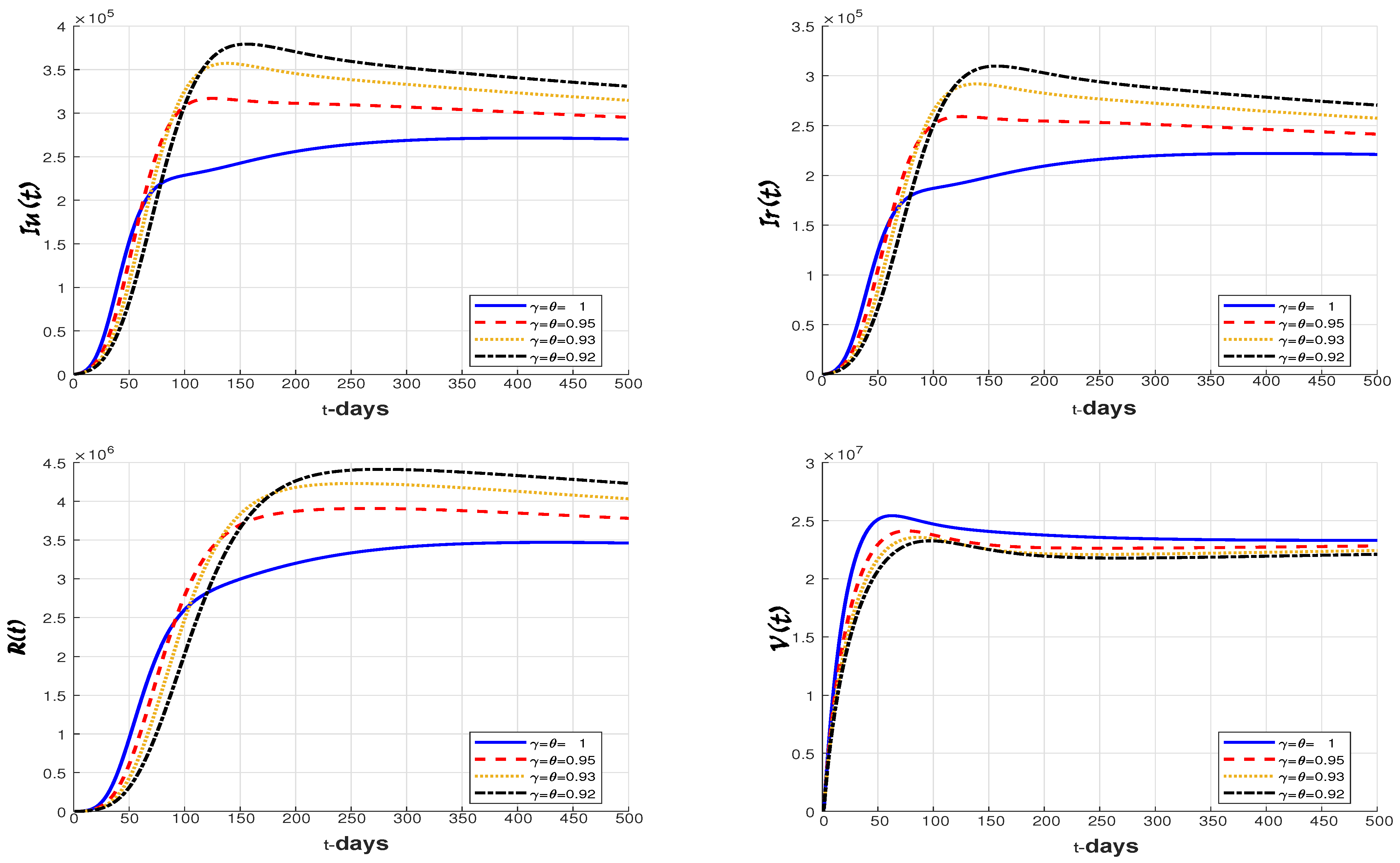
6. Simulations and Discussion

In this section, we employ the numerical scheme (28) to explore simulations of system (1). Given the parameter values listed in Table 1 and the initial conditions S ( 0 ) = 34 , 813 , 051 , V ( 0 ) = 2000 ,   A ( 0 ) = 1500 ,   I u = 204 ,   I r = 80 ,   and R ( 0 ) = 0 , we discuss the influence of fractal and fractional orders, as well as various values of the contact and vaccination parameters, on the dynamics of COVID-19 disease transmission.
Figure 3, Figure 4 and Figure 5 illustrate the numerical results depicting the impact of fractal and fractional orders on the dynamics of COVID-19 disease transmission. It is noted that the populations in the susceptible subclass decrease, while they increase in the remaining five groups over time.
In Figure 3, we fix the fractional order γ = 1 and observe the behavior of the six groups of the model under the impact of different values of the fractal dimension θ = 1 , 0.97 , 0.95 , 0.93 . When the fractal dimension is smaller, both the decrease and increase rates in the susceptible group and the other five groups are slower when compared to higher values of θ .
Figure 4 displays the numerical graphics of the six groups of the model when fixing the fractal dimension θ = 1 and varying the fractional order γ = 1 , 0.97 , 0.95 , 0.93 ; we see that for smaller values of the fractional order γ , the rates of decline in the susceptible group and the growth in the vaccinated group are slower compared with large values of gamma, while smaller values of γ lead to rapid growth in the subclasses of exposed, asymptomatic infected, symptomatic infected, and recovered.
We observe the same behavior in Figure 5, when we vary both the fractal dimension and fractional order together. However, the deceleration of decay and growth rates in the six subclasses is more pronounced compared to the previous case.
This observation demonstrates the feasibility of using fractal–fractional derivatives to enhance the comprehension of the dynamics of a disease.
In this part of the simulation, we explore effective strategies to control the spread of COVID-19. In this regard, we set the values of the fractal dimension and the fractional order to θ = 0.93 and γ = 0.92 , respectively, and observe the influence of varying values of ς , ω V , ω S , and k on the infected populations.
First, we examine the effect of lock-down on the transmission of the coronavirus by changing the contact rate ς . As shown in Figure 6, we note that restricting interactions between susceptible individuals and both asymptomatic and symptomatic infected individuals can decrease the number of future infection cases.
Next, to demonstrate the influence of vaccination, we present the numerical results of the proposed model in Figure 7, both with and without the vaccination parameters. It is observed that there is a clear decrease in the number of infections when vaccine parameters are included.
Figure 8, Figure 9 and Figure 10 depict the influence of the k , ω V and ω S parameter values individually, in order to investigate the optimal approach for implementing vaccination within the community.
In Figure 7, we observe the impact of an increasing vaccination rate ( ω V ) on the size of the infected groups. It becomes evident that as the vaccination rate rises, the number of infections decreases over time.
Figure 9 displays the evolution of the number of infections under improved vaccine effectiveness. It must be noted first that if k is close to 0, the vaccine is more effective. It is observed that as the vaccine’s effectiveness increases, the number of infected individuals decreases.
Figure 10 depicts the impact of the vaccine’s waning immunity rate, and we see that the number of infections decreases significantly when we take smaller values of ω S .
Then, we can conclude that by increasing both the vaccination rate ( ω V ) and vaccine efficacy (k) while decreasing the waning immunity rate ( ω S ) , we can achieve a rapid reduction in the number of infected cases within the population.
To validate this conclusion, Figure 11 presents numerical results obtained by increasing the vaccination rate from 0.0428 to 0.0488 and decreasing the waning immunity rate from 0.01 to 0.009. It is evident that the reduction in the number of infected cases occurs more rapidly when compared to the results shown in Figure 7.

7. Conclusions

This research presents a developed model of COVID-19 virus transmission. We used fractal–fractional derivatives to create a suitable model of the third wave of COVID-19 in the KSA. The qualitative examination of the suggested model began with showing the existence and uniqueness of solutions as provided by the Perov fixed point theorem. Furthermore, we demonstrated the stability of the suggested system’s solutions using Ulam–Hyers principles. In addition, the numerical approach for the model was provided using the two-step Newton polynomial approximation. Then, by adjusting the fractal dimension values, fractional order, contact rate, vaccination rate, and loss of immunity rate, we graphed the convergence and stability of the system’s six solutions. Using our results, better responses will be implemented in the following waves, which will help eliminate the disease forever from society.
Our study did, however, have some limitations. First, the hospitalization class was not taken into account in this study. Additionally, the vaccination process typically consists of three stages: the first dose, the second dose, and the booster dose. Therefore, it is necessary to divide the vaccinated segment into three subclasses. Furthermore, while our study provides insights into the dynamics of infection rates in relation to vaccination strategies, we acknowledge its limitations. Primarily, it does not encompass the broader implications of vaccination, such as the impact on mortality rates. Further research is warranted to explore this critical aspect, especially in light of emerging data that suggest complex outcomes of vaccination programs in terms of public health. Future studies should aim to integrate comprehensive mortality rate analyses, comparing vaccinated and unvaccinated populations, to provide a more holistic understanding of vaccine efficacy and public health implications.

Author Contributions

Validation, F.K.A., investigation, F.K.A., M.H.A. and M.M.; writing—review & editing, F.K.A.; methodology, F.K.A., M.H.A.; data curation, F.K.A. and M.H.A.; formal analysis, M.H.A., N.L. and M.M.; resources, N.L.; writing—original draft preparation, A.B. and M.M.; visualization, N.L.; supervision, A.B.; software, M.M. All authors have read and agreed to the published version of the manuscript.

Funding

This work was funded by the Najran University, Najran, Saudi Arabia, under grant code (NU/NRP/SERC/12/3).

Data Availability Statement

Data is available from the corresponding author on a reasonable request.

Acknowledgments

The authors are thankful to the Deanship of Scientific Research at Najran University for funding this work under the Research Priorities and Najran Research funding program, grant code NU/NRP/SERC/12/3.

Conflicts of Interest

The authors declare that they have no known competing financial interests or personal relationships that could have appeared to influence the work reported in this paper.

References

  1. Podlubny, I. Fractional Differential Equations: An Introduction to Fractional Derivatives, Fractional Differential Equations, to Methods of Their Solution and Some of Their Applications; Elsevier: Amsterdam, The Netherlands, 1998. [Google Scholar]
  2. El hadj Moussa, Y.; Boudaoui, A.; Ullah, S.; Bozkurt, F.; Abdeljawad, T.; Alqudah, M.A. Stability analysis and simulation of the novel Corornavirus mathematical model via the Caputo fractional-order derivative: A case study of Algeria. Results Phys. 2021, 26, 104324. [Google Scholar] [CrossRef] [PubMed]
  3. Sun, T.C.; DarAssi, M.H.; Alfwzan, W.F.; Khan, M.A.; Alqahtani, A.S.; Alshahrani, S.S.; Muhammad, T. Mathematical Modeling of COVID-19 with Vaccination Using Fractional Derivative: A Case Study. Fractal Fract. 2023, 7, 234. [Google Scholar] [CrossRef]
  4. Ambikapathy, B.; Krishnamurthy, K. Mathematical modelling to assess the impact of lockdown on COVID-19 transmission in india: Model development and validation. JMIR Public Health Surveill. 2020, 6, e19368. [Google Scholar] [CrossRef] [PubMed]
  5. Nkambaa, L.N.; Manyombeb, M.L.M.; Mangac, T.T.; Mbangb, J. Modeling analysis of a seiqr epidemic model to assess the impact of undetected cases, and predict the early peack of the COVID-19 outbreak in cameroon. Lond. J. Res. Sci. 2020. [Google Scholar] [CrossRef]
  6. Ullah, S.; Khan, M.A. Modeling the impact of non-pharmaceutical interventions on the dynamics of novel coronavirus with optimal control analysis with a case study. Chaos Solitons Fractals 2020, 139, 110075. [Google Scholar] [CrossRef] [PubMed]
  7. Alqarni, M.S.; Alghamdi, M.; Muhammad, T.; Alshomrani, A.S.; Khan, M.A. Mathematical modeling for novel coronavirus (COVID-19) and control. Numer. Methods Partial. Differ. Equ. 2020, 38, 760–776. [Google Scholar] [CrossRef] [PubMed]
  8. Almeida, R.; Brito da Cruz, A.M.; Martins, N.; Monteiro, M.T.T. An epidemiological mseir model described by the caputo fractional derivative. Int. J. Dyn. Control 2019, 7, 776–784. [Google Scholar] [CrossRef]
  9. Ullah, S.; Khan, M.A.; Farooq, M. A fractional model for the dynamics of tb virus. Chaos Solitons Fractals 2018, 116, 63–71. [Google Scholar] [CrossRef]
  10. Awais, M.; Alshammari, F.S.; Ullah, S.; Khan, M.A.; Islam, S. Modeling and simulation of the novel coronavirus in caputo derivative. Results Phys. 2020, 19, 103588. [Google Scholar] [CrossRef] [PubMed]
  11. Naik, P.A.; Yavuz, M.; Qureshi, S.; Zu, J.; Townley, S. Modeling and analysis of COVID-19 epidemics with treatment in fractional derivatives using real data from pakistan. Eur. Phys. J. Plus 2020, 135, 795. [Google Scholar] [CrossRef] [PubMed]
  12. Safare, K.M.; Betageri, V.S.; Prakasha, D.G.; Veeresha, P.; Kumar, S. A mathematical analysis of ongoing outbreak COVID-19 in India through non singular derivative. Numer. Methods Partial. Differ. Equ. 2020, 37, 1282–1298. [Google Scholar] [CrossRef]
  13. Kumar, S.; Chauhan, R.P.; Momani, S.; Hadid, S. Numerical investigation on COVID-19 model through singular and non-singular fractional operators. Numer. Methods Partial. Differ. Equ. 2020, 40, e22707. [Google Scholar] [CrossRef]
  14. Khan, M.A.; Ullah, S.; Kumar, S. A robust study on 2019-nCOV outbreaks through non-singular derivative. Eur. Phys. J. Plus 2021, 136, 168. [Google Scholar] [CrossRef] [PubMed]
  15. Atangana, A. Fractal-fractional differentiation and integration: Connecting fractal calculus and fractional calculus to predict complex system. Chaos Solitons Fractals 2017, 102, 396–406. [Google Scholar] [CrossRef]
  16. Atangana, A.; Qureshi, S. Modeling attractors of chaotic dynamical systems with fractal-fractional operators. Chaos Solitons Fractals 2019, 123, 320–337. [Google Scholar] [CrossRef]
  17. Perov, A. On the Cauchy problem for a system of ordinary differential equations, Priblijen. Pviblizhen. Met. Reshen. Differ. Uvavn 1964, 2, 115–134. [Google Scholar]
  18. Khan, A.; Zarin, R.; Hussain, G.; Ahmad, N.A.; Mohd, M.H.; Yusuf, A. Stability analysis and optimal control of COVID-19 with convex incidence rate in khyber pakhtunkhawa (pakistan). Results Phys. 2020, 20, 103703. [Google Scholar] [CrossRef] [PubMed]
  19. Saudi Arabia Population 1950–2024. Available online: https://www.worldometers.info/world-population/saudi-arabia-population/ (accessed on 27 March 2023).
  20. Urs, C. Ulam-Hyers stability for coupled fixed points of contractive type operators. J. Nonlinear Sci. Appl. 2013, 6, 124–136. [Google Scholar]
  21. Atangana, A.; İǧret Araz, S. New Numerical Scheme with Newton Polynomial: Theory, Methods, and Applications; Academic Press: Cambridge, MA, USA, 2021. [Google Scholar]
Figure 1. Flow diagram showing the transmission between different compartments.
Fractalfract 08 00095 g001
Figure 2. Curve fitted (solid blue line) to the confirmed infected cases in the KSA in the period between 16 December 2022 and 8 February 2023.
Fractalfract 08 00095 g002
Figure 3. Numerical results for model (6) under various values of the fractal dimension θ .
Fractalfract 08 00095 g003
Figure 4. Numerical results for model (6) under various values of the fractional order γ .
Fractalfract 08 00095 g004
Figure 5. Numerical results for model (6) under various values of the fractal–fractional dimension θ ,   γ .
Fractalfract 08 00095 g005aFractalfract 08 00095 g005b
Figure 6. The impact of the contact rate on the components of the system.
Fractalfract 08 00095 g006aFractalfract 08 00095 g006b
Figure 7. The dynamic behavior of the infected population with and without vaccination ( ω V = 0.0458 ,   ω S = 0.01 ,   k = 0.2851 ).
Fractalfract 08 00095 g007
Figure 8. The impact of the vaccination rate on the components of the infected classes.
Fractalfract 08 00095 g008
Figure 9. The impact of the vaccination efficacy rate on the components of the infected classes.
Fractalfract 08 00095 g009
Figure 10. The impact of the loss of immunity rate on the components of the infected classes.
Fractalfract 08 00095 g010
Figure 11. Numerical results for the behavior of the infected population with and without vaccination ( ω V = 0.0488 ,   ω S = 0.009 ,   k = 0.2851 ).
Fractalfract 08 00095 g011
Table 1. Definitions of parameters used in model (4) and their values in numerical simulations.
SymbolDefinitionValueReference
Λ Birth rate in susceptible class 1273.94 Estimated [19]
ω 2 Natural immunity loss of the recovered individuals 0.0458 Fitted
ω V Vaccine rate of healthy individuals 0.0428 Fitted
ω S Dwindling vaccination immunity rate 0.0100 Fitted
ς Effective contact rate 0.8900 Fitted
ϵ Coefficient of symptomatic individuals 0.0020 Fitted
mNatural mortality rate 0.7989 Estimated [19]
kVaccination efficacy 0.2851 Fitted
ρ Incubation time period 0.8000 Fitted
σ Proportion joining the class symptomatically infected 0.4240 Fitted
v u Recovery rate of asymptomatic people 0.3380 Fitted
v r Recovery of symptomatic people 0.3032 Fitted
d 1 Death rate due to coronavirus in the asymptomatic class1.1140 × 10−4Fitted
d 2 Death rate due to coronavirus in the symptomatic class 0.0011 Fitted
Disclaimer/Publisher’s Note: The statements, opinions and data contained in all publications are solely those of the individual author(s) and contributor(s) and not of MDPI and/or the editor(s). MDPI and/or the editor(s) disclaim responsibility for any injury to people or property resulting from any ideas, methods, instructions or products referred to in the content.

