Article

Theoretical and Numerical Simulations on the Hepatitis B Virus Model through a Piecewise Fractional Order

by
K. A. Aldwoah
1,†,
Mohammed A. Almalahi
2,*,† and
Kamal Shah
3,4,*,†
1
Department of Mathematics, Faculty of Science, Islamic University of Madinah, Al Madinah 42351, Saudi Arabia
2
Department of Mathematics, Hajjah University, Hajjah 00967, Yemen
3
Department of Mathematics, University of Malakand, Chakdara Dir(L) 18000, Khyber Pakhtunkhawa, Pakistan
4
Department of Computer Science and Mathematics, Lebanese American University, Byblos P.O. Box 36, Lebanon
*
Authors to whom correspondence should be addressed.
These authors contributed equally to this work.
Fractal Fract. 2023, 7(12), 844; https://doi.org/10.3390/fractalfract7120844
Submission received: 27 October 2023 / Revised: 18 November 2023 / Accepted: 25 November 2023 / Published: 28 November 2023

Abstract

:
In this study, we introduce the dynamics of a Hepatitis B virus (HBV) model with the class of asymptomatic carriers and conduct a comprehensive analysis to explore its theoretical aspects and examine the crossover effect within the HBV model. To investigate the crossover behavior of the operators, we divide the study interval into two subintervals. In the first interval, the classical derivative is employed to study the qualitative properties of the proposed system, while in the second interval, we utilize the ABC fractional differential operator. Consequently, the study is initiated using the piecewise Atangana–Baleanu derivative framework for the systems. The HBV model is then analyzed to determine the existence, Hyers–Ulam (HU) stability, and disease-free equilibrium point of the model. Moreover, we showcase the application of an Adams-type predictor-corrector (PC) technique for Atangana–Baleanu derivatives and an extended Adams–Bashforth–Moulton (ABM) method for Caputo derivatives through numerical results. Subsequently, we employ computational methods to numerically solve the models and visually present the obtained outcomes using different fractional-order values. This network is designed to provide more precise information for disease modeling, considering that communities often interact with one another, and the rate of disease spread is influenced by this factor.
MSC:
34D20; 37M05; 37N25; 92D30; 34A40

1. Introduction

Hepatitis B is a severe liver infection caused by a virus. This inflammation poses a significant global health challenge. The viral infection, known as hepatitis B, can lead to both acute and chronic illnesses. The primary mode of transmission is from an infected mother to her child during pregnancy, childbirth, or delivery. It can also spread through contact with infected individuals’ blood or other bodily fluids, such as through sexual contact, unsafe injections, or exposure to contaminated medical or public objects. Individuals who inject drugs are also at risk.
According to estimates from the World Health Organization (WHO) [1], approximately 296 million individuals worldwide have chronic hepatitis B, as indicated by the presence of hepatitis B surface antigen. In 2019 alone, around 820,000 people died from hepatitis B, with most deaths attributed to cirrhosis and primary liver cancer (hepatocellular carcinogenesis). Only 6.6 million individuals (22% of those diagnosed) were receiving treatment, accounting for approximately 10% of the total infected population.
The WHO reports a significant decline in the prevalence of chronic hepatitis B virus infection among children under the age of five. In the pre-vaccine era (1980s to early 2000s), the estimated rate was around 5%, whereas in 2019, it dropped to less than 1%. However, despite the availability of highly effective vaccines, the WHO still predicts approximately 1.5 million new cases of hepatitis B infection per year.
Scientists worldwide have developed HBV models to assess the effectiveness of different interventions. For example, the HBV model with vaccination campaigns to reduce HBV transmission rates and the overall burden of the disease [2] and, the HBV model with age structure analysis [3] by considering the age distribution of the population and incorporating age-specific factors, such as susceptibility and vaccination rates. On the other hand, they introduced HBV models as a multi-group system [4]. Mathematical modeling also helps quantify the importance of vaccination in controlling HBV transmission [5]. These models estimate the impact of vaccination coverage on reducing HBV incidence, prevalence, and associated complications. By quantifying the potential benefits of vaccination, policymakers can make informed decisions about immunization programs and their impact on public health. Some HBV models incorporate diffusion processes [6]. These models consider how HBV can spread across geographical regions or populations and evaluate the role of migration in shaping the transmission dynamics. By integrating spatial and temporal factors, delay HBV models with time delay [7] account for the time lag between infection, disease progression, and the implementation of control measures. These models capture the impact of delays in diagnosis, treatment initiation, or vaccine effectiveness in HBV transmission dynamics and provide a more realistic representation of the disease dynamics, and help assess the effectiveness of control strategies under different scenarios. The HBV models discussed earlier rely on integer-order derivatives, which fail to capture the genetic and memory characteristics observed in fractional-order models.
Fractional calculus [8,9] has gained significant popularity among researchers due to its applicability in modeling real-world phenomena. Consequently, researchers in mathematical biology have increasingly turned their attention to utilizing fractional-order derivatives for more accurate mathematical modeling. Various operators, including fractal derivative, non-integer order derivative with a kernel of singularity and non-singularity, and fractal-fractional operator have been proposed to address crossover behavior in different fields such as infectious disease models [10,11]. For additional studies on Atangana–Baleanu fractional models, we refer the readers to a series of papers that delve into various aspects of Atangana–Baleanu fractional models and provide valuable insights into the subject matter [12,13,14,15]. Abdeljawad [16,17,18] proposed a new nonsingular fractional derivative in Atangana-Baleanu settings, incorporating a multi-parameter Mittag–Leffler function. Atangana–Seda [19] adopted a novel technique involving piecewise differential and integral operators. Recently, Gul et al. [20] considered the HBV model with class of asymptomatic carriers under the Caputo derivative. Kumar et al. [21] considered the HBV model with a class of asymptomatic carriers through singular and non-singular derivatives. Shah et al. [22] studied the HBV with treatment via Atangana–Baleanu derivative. The models described above studied the qualitative properties of HBV with great success, but no one so far has studied the problem of crossover behaviors of the HBV disease.
The dynamics of disease transmission in the HBV model can vary over different periods due to several factors such as vaccination campaigns, changes in healthcare practices, or variations in population demographics can influence the dynamics of disease transmission. These factors may vary over different time intervals, leading to corresponding changes in disease dynamics. The piecewise ABC fractional operator enables the modeling of such phenomena more accurately [23,24,25,26]. It allows for the description of systems that experience different dynamics, such as growth, decay, or oscillations, in distinct regions or intervals.
In this work, we consider the HBV model and extend the studies mentioned above with piecewise differential and integral operators for the Atangana–Baleanu fractional derivative to study the dynamics of the HBV model with the class of asymptomatic carriers and conduct a comprehensive analysis of theoretical aspects. Additionally, we examine the crossover effect within the HBV model by dividing the study interval into two subintervals. In the first interval, the classical derivative is employed to study the qualitative properties of the HBV model, while in the second interval, we utilize the ABC fractional differential operator to provide insights into how different scales interact and influence overall HBV model behavior.
Here, we remark on the applicability of the considered differential operator. Many real-world issues show transitions between processes; for instance, when going from power law to randomness, the idea of piecewise was presented. Piecewise approaches in fractional order derivatives (FDEs) differ from conventional methods in that they do not involve abrupt jumps or breaks, and as a result, they do not exhibit crossover behavior. Here, the abrupt jump point shows that the phenomenon exhibits a variety of behaviors following a sudden change. Additionally, the time domain is divided into two subintervals in this instance. In contrast to conventional fractional order derivatives, the piecewise concept facilitates the representation of crossover behaviors among various patterns. However, scientists have found that some real-world issues show processes that behave differently over time and space. A transition from power law to exponential decay, or from deterministic to stochastic, is a specific example. Piecewise differential and integral operators were introduced to address problems exhibiting crossover behaviors because it was observed that the differential operators currently in use might not be able to account for these behaviors (see Ref. [19]).
The advantage of the piecewise ABC fractional operator is capturing complex behaviors and phenomena that exhibit different characteristics in different regions or time intervals in improving modeling flexibility by formulation of models that can adapt to different scenarios or regimes within a single framework. In addition, it facilitates the development of efficient approximation methods by the decomposition of a function or system into simpler sub-regions or intervals, where more tractable approximations can be applied.
The structure of our paper is as follows: Section 2 provides essential definitions and results that will be necessary for subsequent discussions. In Section 3, we present a detailed description of the piecewise model. Section 4 is dedicated to studying the fundamental characteristics of the HBV model which encompasses the analysis of a dynamic system of HBV with a class of asymptomatic carriers. We also examine the extinction scenario of the deterministic model in terms of the basic reproduction number. Moving on to Section 5, we delve into the analysis of the fractional-order system. Here, we establish the existence and uniqueness of the solution and investigate the stability of the solution. In Section 6, we provide numerical solutions of the piecewise fractional-order model, while Section 7 focuses on presenting graphical representations of the HBV model. We conclude with some closing remarks that highlight the significance and implications of our work in the field.

2. Basic Concepts

In this section, we present some definitions and basic auxiliary results of piecewise derivative and integral with classical and Mittag–Leffler kernel that are required throughout our paper.
Definition 1
([19]). The piecewise derivative with classical and Mittag–Leffler kernel is given as
0 P A B D t ς η ( ι ) = D 1 η ( ι ) , ι 0 , ι 1 , A B D 0 ς η ( ι ) , ι ι 1 , T ,
where
(i) D 1 η ( ι ) = d d t η ( ι ) is the classical derivative.
(ii) A B D 0 ς η ( ι ) = ( ς ) 1 ς a ι E ς ς ς 1 ι s ς η ( s ) d s is the Atangana–Baleanu fractional derivative. ( η ) is the normalization function with where the property ( 0 ) = ( 1 ) = 1 and E η is the Mittag–Leffler function.
Definition 2
([19]). Let f be continuous. A piecewise integral of f is given as
0 P A B I t ς η ( ι ) = I 1 η ( ι ) , ι 0 , ι 1 , A B I ς η ( ι ) , ι ι 1 , T ,
where
(i) I 1 η ( ι ) = 0 ι η ( s ) d s is the classical integral,
(ii) A B I ς η ( ι ) = 1 ς ( ς ) η ( ι ) + ς ( ς ) Γ ( ς ) ι 1 ι ( ι s ) ς 1 η ( s ) d s is the Atangana–Baleanu integral.
Theorem 1.
Let X be a Banach space. The operator Φ : C J , R + C J , R + is Lipschitzian if there exists a constant 0 < L < 1 such that i.e., Φ ( ) Φ ( * ) L * for all , * C J , R + . Then Φ is a contraction.

3. Mathematical Model

Studying the dynamics of a Hepatitis B virus (HBV) model with asymptomatic carriers is important for understanding disease transmission, developing effective control and prevention strategies, optimizing treatment approaches, and informing public health policies related to HBV. Here, we will consider generalizing the HBV model with class of asymptomatic carriers [20] in the frame of piecewise derivative with classical and Atangana–Baleanu as follows
0 P A B D ι ς S ( ι ) = ϱ ω A + ϕ 1 A c + ϵ 1 C S Λ S , 0 P A B D ι ς E ( ι ) = ω A + ϕ 1 A c + ϵ 1 C S Λ + ψ 1 E , 0 P A B D ι ς A ( ι ) = ψ 1 γ E Λ + μ + η 1 + κ 1 A , 0 P A B D ι ς A c ( ι ) = ψ 1 1 γ E Λ + τ 1 + θ A c , 0 P A B D ι ς C ( ι ) = η 1 A + τ 1 A c Λ + ν + σ 1 C , 0 P A B D ι ς R p ( ι ) = κ 1 A + σ 1 C + θ A c Λ R p .
The parameter ϱ represents the birth rate of susceptible individuals, while the effective contact rate and natural fatality rate are denoted by ω and Λ , respectively. The rate at which exposed individuals become infected is described as ψ 1 1 γ , with a portion of ψ 1 1 γ moving to class A at a rate of ψ 1 γ . Another portion enters class A c and becomes asymptomatically infected. The rates at which individuals in the acute and asymptomatic classes become carriers are η 1 and τ 1 , respectively. The recovery rates for acute, asymptomatic, and carrier individuals are denoted as κ 1 , θ and σ 1 , respectively. The death rates due to the disease in the acute and chronic classes are represented by μ and ν , respectively. The coefficients for asymptomatic and carrier individuals are indicated as ϕ 1 (representing the infectiousness of asymptomatic infections relative to acute infections) and ϵ 1 (representing the infectiousness of carrier infections relative to acute infections), respectively. The total population represented by N ( ι ) is divided into six classes as follows
  • Susceptible individuals S ( ι ) ;
  • Exposed population E ( ι )
  • Acute infected population A ( ι ) ;
  • Asymptomatic carrier A c ( ι ) ;
  • Chronic infected individuals C ( ι ) ;
  • Recovered population R p ( ι ) .
The total population N ( ι ) = S ( ι ) + E ( ι ) + A ( ι ) + A c ( ι ) + C ( ι ) + R p ( ι ) . with initial conditions S ( 0 ) > 0 ,   E ( 0 ) > 0 ,   A ( 0 ) > 0 ,   A c ( 0 ) > 0 ,   C ( 0 ) > 0 and R p ( 0 ) > 0 . To investigate the crossover behavior of the operators, we divide the study interval 0 , T into two subintervals 0 , ι 1 and ι 1 , T for 0 < ς < 1 , the model (1) can be rewritten as
0 P A B D ι ς S ( ι ) = d d ι W 1 ( ι ,   S ,   E ,   A ,   A c ,   C ,   R p ) ,   ι 0 ,   ι 1 , A B D 0 ς W 1 ( ι ,   S ,   E ,   A ,   A c ,   C ,   R p ) ,   ι ι 1 ,   T ,
0 P A B D ι ς E ( ι ) = d d ι W 2 ( ι ,   S ,   E ,   A ,   A c ,   C ,   R p ) ,   ι 0 ,   ι 1 , A B D 0 ς W 2 ( ι ,   S ,   E ,   A ,   A c ,   C ,   R p ) ,   ι ι 1 ,   T ,
0 P A B D ι ς A ( ι ) = d d ι W 3 ( ι ,   S ,   E ,   A ,   A c ,   C ,   R p ) ,   ι 0 ,   ι 1 , A B D 0 ς W 3 ( ι ,   S ,   E ,   A ,   A c ,   C ,   R p ) ,   ι ι 1 ,   T ,
0 P A B D ι ς A C ( ι ) = d d ι W 4 ( ι ,   S ,   E ,   A ,   A c ,   C ,   R p ) ,   ι 0 ,   ι 1 , A B D 0 ς W 4 ( ι ,   S ,   E ,   A ,   A c ,   C ,   R p ) ,   ι ι 1 ,   T ,
0 P A B D ι ς C ( ι ) = d d ι W 5 ( ι ,   S ,   E ,   A ,   A c ,   C ,   R p ) ,   ι 0 ,   ι 1 , A B D 0 ς W 5 ( ι ,   S ,   E ,   A ,   A c ,   C ,   R p ) ,   ι ι 1 ,   T ,
0 P A B D ι ς R p ( ι ) = d d ι W 6 ( ι ,   S ,   E ,   A ,   A c ,   C ,   R p ) ,   ι 0 ,   ι 1 , A B D 0 ς W 6 ( ι ,   S ,   E ,   A ,   A c ,   C ,   R p ) ,   ι ι 1 ,   T ,
where d d ι and A B D 0 ς are classical and Atangana–Baleanu derivatives, respectively, and
W 1 ( ι ,   S ,   E ,   A ,   A c ,   C ,   R p ) = ϱ ω A + ϕ 1 A c + ϵ 1 C S Λ S , W 2 ( ι ,   S ,   E ,   A ,   A c ,   C ,   R p ) = ω A + ϕ 1 A c + ϵ 1 C S Λ + ψ 1 E , W 3 ( ι ,   S ,   E ,   A ,   A c ,   C ,   R p ) = ψ 1 γ E Λ + μ + η 1 + κ 1 A , W 4 ( ι ,   S ,   E ,   A ,   A c ,   C ,   R p ) = ψ 1 1 γ E Λ + τ 1 + θ A c , W 5 ( ι ,   S ,   E ,   A ,   A c ,   C ,   R p ) = η 1 A + τ 1 A c Λ + ν + σ 1 C , W 6 ( ι ,   S ,   E ,   A ,   A c ,   C ,   R p ) = κ 1 A + σ 1 C + θ A c Λ R p .
For further analysis, we can represent the model (5) as follows
0 P A B D ι ς ( ι ) = d d ι G ( ι ,   ( ι ) ) ,   ι 0 ,   ι 1 , A B D 0 ς G ( ι ,   ( ι ) ) ,   ι ι 1 ,   T ,
where
( ι ) = S ( ι ) ,   E ( ι ) ,   A ( ι ) ,   A c ( ι ) ,   C ( ι ) ,   R p ( ι ) T ,
and
G ( ι , ( ι ) ) = W 1 ( ι , S , E , A , A c , C , R p ) W 2 ( ι , S , E , A , A c , C , R p ) W 3 ( ι , S , E , A , A c , C , R p ) W 4 ( ι , S , E , A , A c , C , R p ) W 5 ( ι , S , E , A , A c , C , R p ) W 6 ( ι , S , E , A , A c , C , R p ) .
The solution of piecewise Atangana–Baleanu model (8) with conditions
( 0 ) = S 0 , E 0 , A 0 , A c 0 , C 0 , R p 0 T > 0 ,
is given by [19]
( ι ) = ( 0 ) + 0 ι G ( σ , ( σ ) ) d σ ,   i f   ι 0 , ι 1 , ( ι 1 ) + 1 ς ( ς ) G ( ι , ( ι ) ) + ς ( ς ) Γ ( ς ) ι 1 ι ( ι σ ) ς 1 G ( σ , ( σ ) ) d σ ,   i f   ι ι 1 , T .

4. Fundamental Characteristics of the HBV Model (1)

In this section, we will study the fundamental characteristics of the HBV model (1), which incorporates the study of a dynamic system of HBV with a class of asymptomatic carriers. Some new perspectives of fractional calculus are established based on the following outcomes: The identification of an invariant region, positivity of solutions, equilibrium and endemic points, basic reproduction number, local and global stability, and sensitivity indices to the model parameters.

4.1. Non-Negativity and Boundedness of the Solutions

In this subsection, we discuss the effects of awareness on the transmission dynamics of HBV model, represented by S , E , A , A c , C and R p , which will be analyzed within a biologically and mathematically feasible region. In the following theorems, we demonstrate the boundedness and positivity of solutions for the piecewise HBV model (1) within a viable region Ω where
Ω = S , E , A , A c , C , R p ; S + E + A + A c + C + R p ϱ Λ .
Theorem 2.
All solutions of model (1) are bounded in the region  Ω .
Proof. 
At the time ι , the piecewise derivative of the total population N ( ι ) is
0 P A B D ι ς N ( ι ) = 0 P A B D ι ς S ( ι ) + 0 P A B D ι ς E ( ι ) + 0 P A B D ι ς A ( ι ) + 0 P A B D ι ς A c ( ι ) + 0 P A B D ι ς C ( ι ) + 0 P A B D ι ς R p ( ι ) = ϱ Λ S + E + A + A c + C + R p μ A + κ 1 A + κ 1 A ν C = ϱ Λ N ( ι ) μ A + κ 1 A + κ 1 A ν C ,
where
N ( ι ) = S ( ι ) + E ( ι ) + A ( ι ) + A c ( ι ) + C ( ι ) + R p ( ι ) .
Clearly
ϱ Λ N ( ι ) μ A + κ 1 A + κ 1 A ν C ϱ Λ N ( ι ) .
From (10), we have
0 P A B D ι ς N ( ι ) ϱ Λ N ( ι ) .
By Definition 1, the inequality (10), becomes
d d ι N ( ι ) ϱ Λ N ( ι ) , ι 0 , ι 1 , A B D 0 ς N ( ι ) ϱ Λ N ( ι ) , ι ι 1 , T .
Case (1): For ι 0 , ι 1 , we have
d d ι N ( ι ) ϱ Λ N ( ι ) .
Thus
N ( ι ) N ( 0 ) e Λ ι + ϱ Λ 1 e Λ ι .
Consequently, N ( ι ) bounded by ϱ Λ in case ι 0 , ι 1 .
Case (2): For ι ι 1 , T , we have
A B D 0 ς N ( ι ) ϱ Λ N ( ι ) .
We apply the Laplace transform on both sides of (11) and obtain
L A B D 0 ς N ( ι ) s ϱ s Λ L N h ( ι ) s .
By simplification, we get
s N ( s ) s + ς 1 s + Λ N h ( s ) ϱ s 1 + N ( 0 ) s + ς 1 s ,
where N ( s ) = L N ( ι ) s and N ( 0 ) is N at ι = 0 . Hence
N ( s ) ϱ s 1 s + ς 1 s + N ( 0 ) 1 + Λ Λ ς s + Λ ς ϱ 1 ς + ϱ s 1 ς + N ( 0 ) 1 + Λ Λ ς s + Λ ς .
Further simplification yields us
N ( s ) ϱ 1 ς s 0 1 + Λ Λ ς s + Λ ς 1 + Λ Λ ς + ϱ ς s 1 2 1 + Λ Λ ς s + Λ ς 1 + Λ Λ ς + N ( 0 ) 1 + Λ Λ ς s + Λ ς 1 + Λ Λ ς .
Applying the inverse Laplace transformation, we have
N ( ι ) ϱ 1 ς s 0 1 + Λ Λ ς E 1 , 1 M ι + ϱ ς 1 + Λ Λ ς ι E 1 , 2 M ι + N ( 0 ) 1 + Λ Λ ς E 1 , 1 M ι ,
where M = Λ ς 1 + Λ Λ ς and E α , β is the Mittag–Leffler function with two parameters α , β > 0 . We utilize the asymptotic behavior of the Mittag–Leffler function in the inequality (12). As ι , we conclude that N ( ι ) ϱ Λ . Consequently, N ( ι ) bounded by ϱ Λ in case ι ι 1 , T .
From the above cases, we conclude that N ( ι ) bounded by ϱ Λ for ι 0 , T . Hence, the state variables S , E , A , A c , C , R p of the model (1) are bounded within the region Ω . □
Theorem 3.
For the specified set of non-negative with initial conditions S ( 0 ) > 0 , E ( 0 ) > 0 , A ( 0 ) > 0 , A c ( 0 ) > 0 , C ( 0 ) > 0 and R p ( 0 ) > 0 , the solutions of the model (1) are positive.
Proof. 
Let us examine the third equation of model (1), which can be expressed as follows
0 P A B D ι ς A ( ι ) = ψ 1 γ E Λ + μ + η 1 + κ 1 A .
Then, we have
0 P A B D ι ς A ( ι ) Λ + μ + η 1 + κ 1 A ,
By Definition 1, the inequality (13), becomes
d d ι A ( ι ) Λ + μ + η 1 + κ 1 A , ι 0 , ι 1 , A B D 0 ς A ( ι ) Λ + μ + η 1 + κ 1 A , ι ι 1 , T .
Case (1): For ι 0 , ι 1 , we have
d d ι A ( ι ) Λ + μ + η 1 + κ 1 A ,
which on integration gives
A ( ι ) A ( 0 ) exp 0 ι Λ + μ + η 1 + κ 1 A d x > 0 .
This proves the positivity of solution A ( ι ) in case ι 0 , ι 1 .
Case (2): For ι ι 1 , T , we have
A B D 0 ς A ( ι ) Λ + μ + η 1 + κ 1 A .
Let the Λ + μ + η 1 + κ 1 = . Then, we get
A B D 0 ς A ( ι ) A ,
To take the Laplace transform on both sides of (14), we have
s L A ( ι ) s A ( 0 ) s + ς 1 s L A ( ι ) s .
Thus, we get
L A ( ι ) s A ( 0 ) 1 ς s + ς 1 ς .
Applying the inverse Laplace transformation, we have
A ( ι ) A ( 0 ) 1 ς E 1 , 1 ς 1 ς ι .
Since A ( 0 ) > 0 and 0 E 1 , 1 1 , we conclude that A ( ι ) is positive solution in case ι ι 1 , T . Thus, by the above cases we conclude that A ( ι ) is the positive solution for ι 0 , T . By the same techniques, we can prove that the solutions of the model (1) are positive. □

4.2. Equilibrium Point and Basic Reproduction Number

The equilibrium point provides insights into the long-term behavior of a disease, and the basic reproduction number quantifies the potential for disease spread. Both concepts are essential for understanding the dynamics of infectious diseases, evaluating control measures, and making informed decisions in public health interventions. The disease free equilibrium point of the model (1) was obtained by putting equations equal to zero
ϱ ω A + ϕ 1 A c + ϵ 1 C S Λ S = 0 ω A + ϕ 1 A c + ϵ 1 C S Λ + ψ 1 E = 0 ψ 1 γ E Λ + μ + η 1 + κ 1 A = 0 ψ 1 1 γ E Λ + τ 1 + θ A c = 0 η 1 A + τ 1 A c Λ + ν + σ 1 C = 0 κ 1 A + σ 1 C + θ A c Λ R p = 0
Given the above equations, the disease-free equilibrium point of the model (1) is given as
0 = S ( 0 ) , E ( 0 ) , A ( 0 ) , A c ( 0 ) , C ( 0 ) , R p ( 0 ) = ϱ Λ , 0 , 0 , 0 , 0 , 0 ,
where ϱ is birth rate of the susceptible individuals and Λ is the natural fatality rate. From Ref. [27] the nonnegative matrix F and the nonsingular matrix V for the new infection terms and the remaining transfer terms are given by
F = 0 ω ϱ Λ ω ϕ 1 ϱ Λ ω ϵ 1 ϱ Λ 0 0 0 0 0 0 0 0 0 0 0 0 ,
and
V = m 1 0 0 0 γ ψ 1 m 2 0 0 1 γ ψ 1 0 m 3 0 0 η 1 τ 1 m 4 .
Therefore, using the fact R 0 = ρ F V 1 , we obtain the basic reproduction number R 0 for the model (1)
R 0 = ω ϱ γ ψ 1 Λ m 2 m 1 + ω ϕ 1 ϱ ψ 1 1 γ Λ m 3 m 1 + ω ϵ 1 ϱ η 1 γ ψ 1 Λ m 4 m 1 m 2 + ω τ 1 ϱ ψ 1 ϵ 1 1 γ Λ m 4 m 3 m 1 ,
where
m 1 = Λ + ψ 1 , m 2 = Λ + μ + η 1 + κ 1 , m 3 = Λ + τ 1 + θ , m 4 = Λ + ν + σ 1 .

4.3. Endemic Equilibrium Point of the Model (1)

Theorem 4.
The HBV model (1) has a unique positive endemic equilibria provided R 0 > 1
Proof. 
The endemic equilibrium point 1 of the model (1) is given by
1 = S * , E * , A * , A c , C * , R p * ,
where
S * = Λ + ψ 1 A * ω A * + ϕ 1 A c + ϵ 1 C * , E * = Λ + μ + η 1 + κ 1 E * γ ψ 1 , A c * = ψ 1 1 γ E * Λ + τ 1 + θ , C * = η 1 A * + τ 1 A c Λ + ν + σ 1 ,
and
R p * = κ 1 A * + σ 1 C * + θ A c Λ .
Using the above equations in the third equation of the model (1), we get
A * = Λ m 1 m 2 m 3 m 4 γ 1 R 0 ω m 1 m 2 γ m 3 m 4 + η 1 ϵ 1 + 1 γ m 2 m 4 ϕ 1 + τ 1 ϵ 1 ,
where m 1 , m 2 , m 3 and m 4 are defined by (15). Thus, the HBV model (1) has a unique positive endemic equilibria provided R 0 > 1 . □

4.4. Local and Global Stability

Understanding both local and global stability of equilibrium points is important for assessing the behavior and long-term dynamics of infectious diseases. Local stability analysis helps determine whether small perturbations will dampen or amplify, providing insights into the short-term behavior of the system. Global stability analysis, on the other hand, provides guarantees about the long-term behavior, ensuring that the system will reach and remain at the desired equilibrium state. These stability analyses aid in evaluating the effectiveness of control strategies, predicting disease outcomes, and informing public health interventions.
Theorem 5.
The disease-free equilibrium 0 of the HBV model (5) is locally asymptotically stable if R 0 < 1 .
Proof. 
Considering Theorems 2 and 3, it can be concluded that the proof of locally asymptotically stable of the disease-free equilibrium 0 remains unaffected by the presence of the piecewise operator. Consequently, the proof remains by the same technique as the one in Refs. [20,21,22]. Therefore, we omit it here. □
Theorem 6.
If R 0 < 1 and ς 0 , 1 , then the disease free equilibrium 0 of HBV model (5) is globally asymptotically stable on region Ω.
Proof. 
Define the Lyapunov function V by
V = T 1 E ( ι ) + T 2 A ( ι ) + T 3 A c ( ι ) + T 4 A ( ι ) C ( ι ) ,
where T i > 0 , i = 1 , 2 , 3 , 4 is a constant numbers defined as
T 1 = Λ Λ + μ + η 1 + κ 1 Λ + τ 1 + θ Λ + ν + σ 1 , T 2 = ω ϱ Λ + τ 1 + θ Λ + ν + σ 1 + η 1 ϵ 1 , T 3 = ω ϱ Λ + μ + η 1 + κ 1 ϕ 1 Λ + ν + σ 1 + τ 1 ϵ 1 , T 4 = ω ϱ ϵ 1 Λ + μ + η 1 + κ 1 Λ + τ 1 + θ .
We apply the piecewise fractional derivative on both sides of the above equation and get
0 P A B D ι ς V = 0 P A B D ι ς T 1 E ( ι ) + 0 P A B D ι ς T 2 A ( ι ) + 0 P A B D ι ς T 3 A c ( ι ) + 0 P A B D ι ς T 4 C ( ι ) = T 1 ω A + ϕ 1 A c + ϵ 1 C S Λ + ψ 1 E + T 2 ψ 1 γ E Λ + μ + η 1 + κ 1 A + T 3 ψ 1 1 γ E Λ + τ 1 + θ A c + T 4 η 1 A + τ 1 A c Λ + ν + σ 1 C .
Since E ( ι ) , A ( ι ) , A c ( ι ) , and C ( ι ) are positive, then
0 P A B D ι ς V T 2 ψ 1 γ T 1 Λ + ψ 1 + T 3 ψ 1 1 γ E + T 1 ω S 0 T 2 Λ + μ + η 1 + κ 1 + T 4 η 1 A + T 1 ϕ 1 S 0 T 3 Λ + τ 1 + θ + T 4 τ 1 A c + T 1 ω ϵ 1 S 0 T 4 Λ + ν + σ 1 C .
By (17), the inequality (17) becomes
0 P A B D ι ς V Λ Λ + ψ 1 Λ + μ + η 1 + κ 1 Λ + τ 1 + θ Λ + ν + σ 1 R 0 1 E .
If R 0 < 1 , then 0 P A B D ι ς V becomes negative. Thus, the HBV model (5) is globally asymptotically stable. □

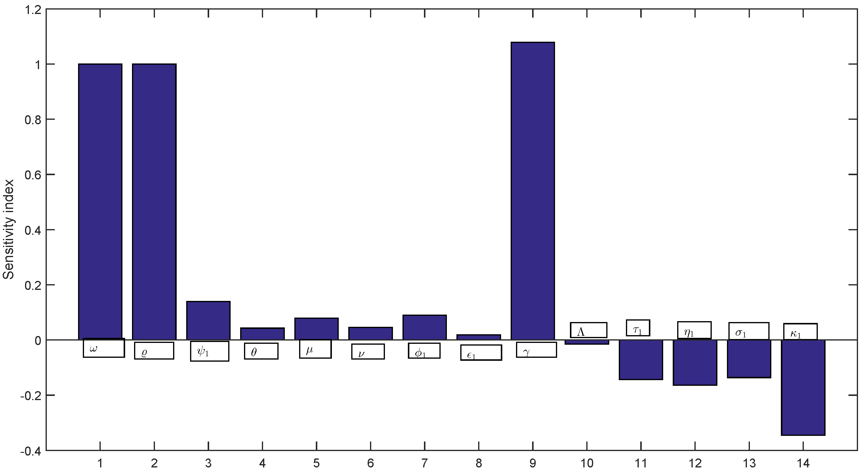
4.5. Sensitivity Analysis

The sensitivity indices play a crucial role in understanding the importance of parameters in the model disease. They guide parameter ranking, uncertainty analysis, model refinement, policy evaluation, and provide insights into the system’s behavior. By utilizing sensitivity analysis techniques. In this subsection, the reproductive number R 0 and sensitivity indices to the model parameters are computed. These indices highlight the importance of every factor in the occurrence and spread of disease. Sensitivity analysis is employed to assess the resistance of the model predictions to parameter values. In this sense, we compute sensitivity indices using the following formula
S R 0 = R 0 R 0 .
Applying the above formula gives
S ω R 0 = ω R 0 R 0 ω = 1 > 0 , S ϱ R 0 = ϱ R 0 R 0 ϱ = 1 > 0 , S ψ 1 R 0 = ψ 1 R 0 R 0 ψ 1 = 0.13922 > 0 , S θ R 0 = θ R 0 R 0 θ = 0.0042872 > 0 , S μ R 0 = μ R 0 R 0 μ = 0.007896 > 0 , S ϕ 1 R 0 = ϕ 1 R 0 R 0 ϕ 1 = 0.001001 > 0 , S ϵ 1 R 0 = ϵ 1 R 0 R 0 ϵ 1 = 0.0019 > 0 , S γ R 0 = γ R 0 R 0 γ = 1.078965 > 0 , S Λ R 0 = Λ R 0 R 0 Λ = 0.01477 < 0 , S τ 1 R 0 = τ 1 R 0 R 0 τ 1 = 0.143657 < 0 , S η 1 R 0 = η 1 R 0 R 0 η 1 = 0.163656 < 0 , S σ 1 R 0 = σ 1 R 0 R 0 σ 1 = 0.13634 < 0 , S ν R 0 = ν R 0 R 0 ν = 0.124567 < 0 , S κ 1 R 0 = κ 1 R 0 R 0 κ 1 = 0.345261 < 0 .
Here, we present the sensitivity indices in the given Figure 1.

5. Qualitative Analysis of HBV Model (1)

In this section, we address the existence and uniqueness of the solution as well as stability results for HBV model (1) by utilizing the fixed point technique. Let J = 0 , T R + , we are defining Banach space Ω = C J , R + × C J , R + × C J , R + × C J , R + × C J , R + × C J , R + under the norm
= S , E , A , A c , C , R P = sup S ( ι ) + E ( ι ) + A ( ι ) + A c ( ι ) + C ( ι ) + R P ( ι ) ,
where S , E , A , A c , C , R P C J , R + . To transform the model (8) into the fixed point problem, we define the operator Φ : Ω Ω by
Φ ( ι ) = ( 0 ) + 0 ι G ( σ , ( σ ) ) d σ , ι 0 , ι 1 , ( ι 1 ) + 1 ς ( ς ) G ( ι , ( ι ) ) + ς ( ς ) Γ ( ς ) ι 1 ι ( ι σ ) ς 1 G ( σ , ( σ ) ) d σ , ι ι 1 , T .
The following assumptions must be fulfilled for the analysis of existence, uniqueness, and stability results for the HBV model (1) using the fixed point technique.
H 1 : G : J × Ω R is continuous and there exist two constants τ , η > 0 such that
G ( ι , ( ι ) ) τ + ( ι ) η ,   for   σ J and   Y F .
H 2 : For ι J and 1 , 2 Ω , there exists the constant number O > 0 such that
G ( ι , 1 ( ι ) ) G ( ι , 2 ( ι ) ) O 1 ( ι ) 2 ( ι ) .
For simplicity of the analysis, we use the following notations
A = 1 ς ( ς ) + ( T ι 1 ) ς ( ς ) Γ ( ς ) , χ = 1 ( ι 1 ) 2 ( ι 1 ) .

5.1. Existence of the Solution

In this subsection, we will prove the existence of the solution for the HBV model by using Krasnoselskii fixed point theorem.
Theorem 7.
Suppose that H 1 and H 2 are satisfied. Then, the model (8) has a solution, provided that
0 < max ι 1 η , A η , O ι 1 , χ + 1 ς ( ς ) O < 1 ,
where χ = 1 ( ι 1 ) 2 ( ι 1 ) .
Proof. 
Let Ψ ζ = Ω : ζ be a closed ball with
ζ max ( 0 ) + ι 1 τ 1 ι 1 η , ( ι 1 ) + 1 ς ( ς ) + ( T ι 1 ) ς ( ς ) Γ ( ς ) τ 1 1 ς ( ς ) + ( T ι 1 ) ς ( ς ) Γ ( ς ) η .
We divide the operator Φ defined by (19) into two operators Φ 1 and Φ 2 such that Φ = Φ 1 + Φ 2 , as follows
Φ 1 ( ι ) = ( 0 ) + 0 ι G ( σ , ( σ ) ) d σ , if ι 0 , ι 1 , ( ι 1 ) + 1 ς ( ς ) G ( ι , ( ι ) ) , if ι ι 1 , T .
and
Φ 2 ( ι ) = 0 , if ι 0 , ι 1 , ς ( ς ) Γ ( ς ) ι 1 ι ( ι σ ) ς 1 G ( σ , ( σ ) ) d σ , if ι ι 1 , T .
To apply the fixed point technique with a piecewise fractional operator, we divide the proof into three steps such that any step has two cases, as follows
Step (1) Φ 1 ( ι ) + Φ 2 ( ι ) Ψ ζ .
Case (1): For ι 0 ,   ι 1 , Ψ ζ , with (H 1 ), we have
Φ 1 ι + Φ 2 ι = sup ι 0 , ι 1 ( 0 ) + 0 ι G ( σ , ( σ ) ) d σ ( 0 ) + 0 ι G ( σ , ( σ ) ) d σ ( 0 ) + ι τ + ι η .
Hence
Φ 1 + Φ 2 ( 0 ) + ι 1 τ + η ( 0 ) + ι 1 τ + ι 1 η ( 0 ) + ι 1 τ + ι 1 η ζ ζ .
Case (2): For ι ι 1 , T , Ψ ζ , we have
Φ 1 ι + Φ 2 ι = sup ι ι 1 , T ( ι 1 ) + 1 ς ( ς ) G ( ι , ( ι ) ) + ς ( ς ) Γ ( ς ) ι 1 ι ( ι σ ) ς 1 G ( σ , ( σ ) ) d σ ( ι 1 ) + 1 ς ( ς ) G ( ι , ( ι ) ) + ς ( ς ) Γ ( ς ) ι 1 ι ( ι σ ) ς 1 G ( σ , ( σ ) ) d σ .
By (H 1 ), we have
Φ 1 ι + Φ 2 ι ( ι 1 ) + 1 ς ( ς ) τ + ( ι ) η + ς ( ς ) Γ ( ς ) ι 1 ι ( ι σ ) ς 1 τ + ( σ ) η d σ .
Hence
Φ 1 + Φ 2 ( ι 1 ) + A τ + A η ζ ζ .
This demonstrates that Φ 1 ( ι ) + Φ 2 ( ι ) Ψ ζ .
Step (2) Φ 1 is contraction.
Case (1): For ι 0 , ι 1 , 1 , 2 Ψ ζ . Then via ( H 2 ) , we get
Φ 1 1 ( ι ) Φ 1 2 ( ι ) sup ι 0 , ι 1 0 ι G ( σ , 1 ( σ ) ) G ( σ , 2 ( σ ) ) d σ O 0 ι 1 ( σ ) 2 ( σ ) d σ .
Hence
Φ 1 1 Φ 1 2 O ι 1 1 2 .
Case (2): For ι ι 1 , T , 1 , 2 Ψ ζ . Then via ( H 2 ) , we get
Φ 1 1 ( ι ) Φ 1 2 ( ι ) χ + 1 ς ( ς ) G ( ι , 1 ( ι ) ) G ( ι , 2 ( ι ) ) χ + 1 ς ( ς ) O 1 ( ι ) 2 ( ι ) .
Hence
Φ 1 1 Φ 1 2 χ + 1 ς ( ς ) O 1 2 .
By the above cases, we get
Φ 1 1 Φ 1 2 max O ι 1 , χ + 1 ς ( ς ) O 1 2 .
Due to (21), we conclude that Φ 1 is contraction mapping.
Step (3) Φ 2 is relatively compact.
Since G ( ι , ( ι ) ) is continuous, then Φ 2 is continuous. Now, we prove that Φ 2 is uniformly bounded on Ψ ζ . Let Ψ ζ . Then, we have
Case (1): For ι 0 , ι 1 , Ψ ζ , we get directly that Φ 2 is uniformly bounded on Ψ ζ .
Case (2): For ι ι 1 , T , Ψ ζ , then via ( H 1 ) , we get
Φ 2 ( ι ) sup ι ι 1 , T ς ( ς ) Γ ( ς ) ι 1 ι ( ι σ ) ς 1 G ( σ , ( σ ) ) d σ ς ( ς ) Γ ( ς ) ι 1 ι ( ι σ ) ς 1 τ + ( σ ) η d σ .
Hence
Φ 2 ( T ι 1 ) ς ( ς ) Γ ( ς ) τ + ζ η .
Thus, Φ 2 is uniformly bounded on Ψ ζ . Next, we prove that Φ 2 is equicontinuous. Let Ψ ζ . Then, we have
Case (1) For any ι a , ι b 0 , ι 1 , ι a < ι b , we have
Φ 2 ι b Φ 2 ι a = 0 .
Case (2) For any ι a , ι b ι 1 , T , ι a < ι b and Ψ ζ , we have
Φ 2 ι b Φ 2 ι a ς ( ς ) Γ ( ς ) ι 1 ι b ( ι b σ ) ς 1 G ( σ , ( σ ) ) d σ ς ( ς ) Γ ( ς ) ι 1 ι a ( ι a σ ) ς 1 G ( σ , ( σ ) ) d σ 1 ( ς ) Γ ( ς ) ( ι b ι 1 ) ς ( ι b ι a ) ς ( ι a ι 1 ) ς τ + η + 1 ( ς ) Γ ( ς ) ( ι b ι a ) ς τ + ζ η 0   as   ι b ι a .
Thus, Φ 2 is equicontinuous. According to the above analysis together with the Arzela–Ascoli theorem, we deduce that Φ 2 is relatively compact and completely continuous. Thus, by the Krasnoselskii fixed point theorem, Equation (8) has at least one solution. □

5.2. Uniqueness of the Solution

In this subsection, we will prove the uniqueness of the solution for the HBV model by using the Banach contraction principle.
Theorem 8.
Assume that ( H 2 ) holds. If 0 < max O ι 1 , OA < 1 , then, the model (8) has a unique solution.
Proof. 
Taking the operator Φ : Ω Ω defined by (19).
Case (1): For ι 0 , ι 1 , 1 , 2 Ψ ζ with (H 2 ), we have
Φ 1 ( ι ) Φ 2 ( ι ) sup ι 0 , ι 1 0 ι G ( σ , 1 ( σ ) ) G ( σ , 2 ( σ ) ) d σ O 0 ι 1 ( σ ) 2 ( σ ) d σ .
Thus
Φ 1 Φ 2 O ι 1 1 2 .
Case (2): For ι ι 1 , T , 1 , 2 Ψ ζ with (H 2 ), we have
Φ 1 ( ι ) Φ 2 ( ι ) sup ι ι 1 , T 1 ς ( ς ) G ( ι , 1 ( ι ) ) G ( ι , 2 ( ι ) ) + ς ( ς ) Γ ( ς ) ι 1 ι ( ι σ ) ς 1 G ( σ , 1 ( σ ) ) G ( σ , 2 ( σ ) ) d σ 1 ς ( ς ) O 1 ( ι ) 2 ( ι ) + ς O ( ς ) Γ ( ς ) ι 1 ι ( ι σ ) ς 1 1 ( σ ) 2 ( σ ) d σ .
Hence
Φ 1 Φ 2 OA 1 2 ,
where A defined by (20). Thus, Φ is contraction. Consequently, the model (8) has a unique solution. □

5.3. Stability Analysis

Definition 3.
The model (8) is UH stable if there exists a real number Q > 0 such that for each ε > 0 there exists a solution ˜ Ω of the inequality
0 P A B D ι ς ^ ( ι ) G ( ι , ^ ( ι ) ) ε , ι J ,
corresponding to a solution Ω of model (8) with the following condition
( 0 ) = ˜ ( 0 ) ,
such that
˜ Q ε , ι J .
Remark 1.
A function ^ Ω is a solution of the inequality
0 P A B D ι ς ^ ( ι ) G ( ι , ^ ( ι ) ) ε
if and only if there exists a small perturbation z F such that
(i)  z ( ι ) ε , ι J ;
(ii)  0 P A B D ι ς ^ ( ι ) = G ( ι , ^ ( ι ) ) + Z ( ι ) , ι J , where
Z ( ι ) = z 1 ( ι ) , z 2 ( ι ) , z 3 ( ι ) , z 4 ( ι ) , z 5 ( ι ) , z 6 ( ι ) T .
Lemma 1.
Let ^ Ω be a function satisfies the inequalities
0 P A B D ι ς ^ ( ι ) G ( ι , ^ ( ι ) ) ε ,
then ^ satisfies the following integral inequalities
^ ( ι ) ^ ( 0 ) 0 ι G ( σ , ^ ( σ ) ) d σ ι 1 ε , i f ι 0 , ι 1 , ^ ( ι 1 ) + 1 ς ( ς ) G ( ι , ^ ( ι ) ) + ς ( ς ) Γ ( ς )    × ι 1 ι ( ι σ ) ς 1 G ( σ , ^ ( σ ) ) d σ A ε , i f ι ι 1 , T ,
where A is defined by (20).
Proof. 
Indeed by Remark 1, we have
0 P A B D ι ς ^ ( ι ) = G ( ι , ^ ( ι ) ) + Z ( ι ) , ι J .
Then
^ ( ι ) = ^ ( 0 ) + 0 ι 1 G ( σ , ^ ( σ ) ) + Z ( σ ) d σ , ι 0 , ι 1 ,    ^ ( ι 1 ) + 1 ς ( ς ) G ( ι , ^ ( ι ) ) + Z ( ι ) + ς ( ς ) Γ ( ς ) ι 1 ι ( ι σ ) ς 1 G ( σ , ^ ( σ ) ) + Z ( σ ) d σ , ι ι 1 , T .
Case(1): For ι 0 , ι 1 , ^ Ω , it follows that
^ ( ι ) ^ ( 0 ) 0 ι G ( σ , ^ ( σ ) ) d σ 0 ι Z ( σ ) d σ ι 1 ε .
Case(2): For ι ι 1 , T , ^ Ω , it follow that
^ ( ι 1 ) + 1 ς ( ς ) G ( ι , ^ ( ι ) ) + ς ( ς ) Γ ( ς ) ι 1 ι ( ι σ ) ς 1 G ( σ , ^ ( σ ) ) d σ 1 ς ( ς ) Z ( ι ) + ς ( ς ) Γ ( ς ) ι 1 ι ( ι σ ) ς 1 Z ( σ ) d σ A ε .
Theorem 9.
Assume that the conditions of Theorem 8 hold. Then the model (8) is UH stable provided that
0 < max ι 1 O , AO < 1 .
Proof. 
Let ε > 0 and ^ Ω be a function satisfying the inequalities
0 P A B D ι ς ^ ( ι ) G ( ι , ^ ( ι ) ) ε ,
and let Ω be the unique solution of the following model
0 P A B D ι ς ( ι ) = G ( ι , ( ι ) ) .
Now, in the light of Theorem 8, we have
( ι ) = ( 0 ) + 0 ι G ( σ , ( σ ) ) d σ , if ι 0 , ι 1 , ( ι 1 ) + 1 ς ( ς ) G ( ι , ( ι ) ) + ς ( ς ) Γ ( ς ) ι 1 ι ( ι σ ) ς 1 G ( σ , ( σ ) ) d σ , if ι ι 1 , T .
Hence, from (H 2 ) and Lemma 1, we have
Case (1): For ι 0 , ι 1 , we have
^ ( ι ) ( ι ) ^ ( ι ) ( 0 ) 0 ι G ( σ , ( σ ) ) d σ ^ ( ι ) ^ ( 0 ) 0 ι G ( σ , ^ ( σ ) ) d σ + 0 ι G ( σ , ^ ( σ ) ) G ( σ , ( σ ) ) d σ ι 1 ε + O 0 ι ^ ( σ ) ( σ ) d σ .
Hence
^ ι 1 ε + O ι 1 ^ .
Thus
^ ι 1 ε 1 O ι 1 .
Case (2): For ι ι 1 , T , we have
^ ( ι ) ( ι ) ^ ( ι 1 ) + 1 ς ( ς ) G ( ι , ( ι ) ) + ς ( ς ) Γ ( ς ) ι 1 ι ( ι σ ) ς 1 G ( σ , ( σ ) ) d σ ^ ( ι 1 ) + 1 ς ( ς ) G ( ι , ^ ( ι ) ) + ς ( ς ) Γ ( ς ) ι 1 ι ( ι σ ) ς 1 G ( σ , ^ ( σ ) ) d σ + 1 ς ( ς ) G ( ι , ^ ( ι ) ) G ( ι , ( ι ) ) + ς ( ς ) Γ ( ς ) ι 1 ι ( ι σ ) ς 1 G ( σ , ^ ( σ ) ) G ( σ , ( σ ) ) d σ A ε + 1 ς ( ς ) O ^ ( ι ) ( ι ) + ς O ( ς ) Γ ( ς ) ι 1 ι ( ι σ ) ς 1 ^ ( σ ) ( σ ) d σ .
Hence
^ A ε + OA ^ .
Thus
^ A ε 1 OA ^ .
By the above cases and by choosing Q > 0 , we get
^ Q ε ,
where
Q = max A ε 1 O ι 1 , A ε 1 O ( ς ) 1 ς + ( T ι 1 ) ς Γ ( ς ) .
This proves that the model (8) is U-H stable. □

6. Numerical Scheme with Piecewise Derivative

Over the past few decades, some analytical and numerical methods have been developed for use in the literature. However, sometimes, especially for large and complicated problems, numerical solutions to differential equations have shown to be more practical and efficient than analytical ones. As a result, scientists have created a variety of numerical techniques to address different types of differential equations with both fractional and ordinary orders. It has been demonstrated by researchers that the Adams–Bashforth method yields good numerical solutions for FDEs along with good stability analysis. Instead, more previously evaluated approximations must be used in multi-step methods to compute the solution. For fractional-order operators, multi-step methods are a natural choice because of their persistent memory for FDEs (we refer to Refs. [28,29,30]). By applying the piecewise integral local and Atangana–Baleanu derivative, we have
S ( ι ) = S ( 0 ) + 0 ι 1 ϱ ω A + ϕ 1 A c + ϵ 1 C S Λ S d σ , S ( ι 1 ) + 1 ς ( ς ) ϱ ω A + ϕ 1 A c + ϵ 1 C S Λ S + ς ( ς ) Γ ( ς ) ι 1 ι ( ι σ ) ς 1 ϱ ω A + ϕ 1 A c + ϵ 1 C S Λ S d σ ,
E ( ι ) = E ( 0 ) + 0 ι 1 ω A + ϕ 1 A c + ϵ 1 C S Λ + ψ 1 E d σ , E ( ι 1 ) + 1 ς ( ς ) ω A + ϕ 1 A c + ϵ 1 C S Λ + ψ 1 E + ς ( ς ) Γ ( ς ) ι 1 ι ( ι σ ) ς 1 ω A + ϕ 1 A c + ϵ 1 C S Λ + ψ 1 E d σ ,
A ( ι ) = A ( 0 ) + 0 ι 1 ψ 1 γ E Λ + μ + η 1 + κ 1 A d σ , A ( ι 1 ) + 1 ς ( ς ) ψ 1 γ E Λ + μ + η 1 + κ 1 A + ς ( ς ) Γ ( ς ) ι 1 ι ( ι σ ) ς 1 ψ 1 γ E Λ + μ + η 1 + κ 1 A d σ ,
A c ( ι ) = A c ( 0 ) + 0 ι 1 ψ 1 1 γ E Λ + τ 1 + θ A c d σ , A c ( ι 1 ) + 1 ς ( ς ) ψ 1 1 γ E Λ + τ 1 + θ A c + ς ( ς ) Γ ( ς ) ι 1 ι ( ι σ ) ς 1 ψ 1 1 γ E Λ + τ 1 + θ A c d σ ,
C ( ι ) = C ( 0 ) + 0 ι 1 η 1 A + τ 1 A c Λ + ν + σ 1 C d σ , C ( ι 1 ) + 1 ς ( ς ) η 1 A + τ 1 A c Λ + ν + σ 1 C + ς ( ς ) Γ ( ς ) ι 1 ι ( ι σ ) ς 1 η 1 A + τ 1 A c Λ + ν + σ 1 C d σ ,
and
R p ( ι ) = R p ( 0 ) + 0 ι 1 κ 1 A + σ 1 C + θ A c Λ R p d σ , R p ( ι 1 ) + 1 ς ( ς ) κ 1 A + σ 1 C + θ A c Λ R p + ς ( ς ) Γ ( ς ) ι 1 ι ( ι σ ) ς 1 κ 1 A + σ 1 C + θ A c Λ R p d σ ,
Now, put ι = ι n + 1 , we get
S ( ι n + 1 ) = S ( 0 ) + 0 ι 1 ϱ ω A + ϕ 1 A c + ϵ 1 C S Λ S d σ , S ( ι 1 ) + 1 ς ( ς ) ϱ ω A + ϕ 1 A c + ϵ 1 C S Λ S + ς ( ς ) Γ ( ς ) ι 1 ι n + 1 ( ι n + 1 σ ) ς 1 ϱ ω A + ϕ 1 A c + ϵ 1 C S Λ S d σ ,
E ( ι n + 1 ) = E ( 0 ) + 0 ι 1 ω A + ϕ 1 A c + ϵ 1 C S Λ + ψ 1 E d σ , E ( ι 1 ) + 1 ς ( ς ) ω A + ϕ 1 A c + ϵ 1 C S Λ + ψ 1 E + ς ( ς ) Γ ( ς ) ι 1 ι n + 1 ( ι n + 1 σ ) ς 1 ω A + ϕ 1 A c + ϵ 1 C S Λ + ψ 1 E d σ ,
A ( ι n + 1 ) = A ( 0 ) + 0 ι 1 ψ 1 γ E Λ + μ + η 1 + κ 1 A d σ , A ( ι 1 ) + 1 ς ( ς ) ψ 1 γ E Λ + μ + η 1 + κ 1 A + ς ( ς ) Γ ( ς ) ι 1 ι n + 1 ( ι n + 1 σ ) ς 1 ψ 1 γ E Λ + μ + η 1 + κ 1 A d σ ,
A c ( ι n + 1 ) = A c ( 0 ) + 0 ι 1 ψ 1 1 γ E Λ + τ 1 + θ A c d σ , A c ( ι 1 ) + 1 ς ( ς ) ψ 1 1 γ E Λ + τ 1 + θ A c + ς ( ς ) Γ ( ς ) ι 1 ι n + 1 ( ι n + 1 σ ) ς 1 ψ 1 1 γ E Λ + τ 1 + θ A c d σ ,
C ( ι n + 1 ) = C ( 0 ) + 0 ι 1 η 1 A + τ 1 A c Λ + ν + σ 1 C d σ , C ( ι 1 ) + 1 ς ( ς ) η 1 A + τ 1 A c Λ + ν + σ 1 C + ς ( ς ) Γ ( ς ) ι 1 ι n + 1 ( ι n + 1 σ ) ς 1 η 1 A + τ 1 A c Λ + ν + σ 1 C d σ ,
and
R p ( ι n + 1 ) = R p ( 0 ) + 0 ι 1 κ 1 A + σ 1 C + θ A c Λ R p d σ , R p ( ι 1 ) + 1 ς ( ς ) κ 1 A + σ 1 C + θ A c Λ R p + ς ( ς ) Γ ( ς ) ι 1 ι n + 1 ( ι n + 1 σ ) ς 1 κ 1 A + σ 1 C + θ A c Λ R p d σ .
By applying the Newton Polynomial interpolation scheme we have
S ( ι n + 1 ) = S ( 0 ) + k = 2 i 5 12 ϱ ω A ι k 2 + ϕ 1 A c ι k 2 + ϵ 1 C ι k 2 S ι k 2 Λ S ι k 2 Δ ι 4 3 ϱ ω A ι k 1 + ϕ 1 A c ι k 1 + ϵ 1 C ι k 1 S ι k 1 Λ S ι k 1 Δ ι + 23 12 ϱ ω A ι k + ϕ 1 A c ι k + ϵ 1 C ι k S ι k Λ S ι k Δ ι , S ( ι 1 ) + 1 ς ( ς ) ϱ ω A ι n + ϕ 1 A c ι n + ϵ 1 C ι n S ι n Λ S ι n + ς Δ ι ς 1 ( ς ) Γ ( ς + 1 ) k = i + 3 n ϱ ω A ι k 2 + ϕ 1 A c ι k 2 + ϵ 1 C ι k 2 S ι k 2 Λ S ι k 2 Φ + ς Δ ι ς 1 ( ς ) Γ ( ς + 1 ) k = i + 3 n ϱ ω A ι k 1 + ϕ 1 A c ι k 1 + ϵ 1 C ι k 1 S ι k 1 Λ S ι k 1 ϱ ω A ι k 2 + ϕ 1 A c ι k 2 + ϵ 1 C ι k 2 S ι k 2 Λ S ι k 2 Σ + ς ( ς ) + ς Δ ι ς 1 2 Γ ( ς + 3 ) k = i + 3 n ϱ ω A ι k + ϕ 1 A c ι k + ϵ 1 C ι k S ι k Λ S ι k 2 ϱ ω A ι k 1 + ϕ 1 A c ι k 1 + ϵ 1 C ι k 1 S ι k 1 Λ S ι k 1 + ϱ ω A ι k 2 + ϕ 1 A c ι k 2 + ϵ 1 C ι k 2 S ι k 2 Λ S ι k 2 Δ ,
E ( ι n + 1 ) = E ( 0 ) + k = 2 i 5 12 ω A ι k 2 + ϕ 1 A c ι k 2 + ϵ 1 C ι k 2 S Λ + ψ 1 E ι k 2 Δ ι 4 3 ω A ι k 1 + ϕ 1 A c ι k 1 + ϵ 1 C ι k 1 S ι k 1 Λ + ψ 1 E ι k 1 Δ ι + 23 12 ω A ι k + ϕ 1 A c ι k + ϵ 1 C ι k S ι k Λ + ψ 1 E ι k Δ ι , E ( ι 1 ) + 1 ς ( ς ) ω A ι n + ϕ 1 A c ι n + ϵ 1 C ι n S ι n Λ + ψ 1 E ι n + ς Δ ι ς 1 ( ς ) Γ ( ς + 1 ) k = i + 3 n ω A ι k 2 + ϕ 1 A c ι k 2 + ϵ 1 C ι k 2 S ι k 2 Λ + ψ 1 E ι k 2 Φ + ς Δ ι ς 1 ( ς ) Γ ( ς + 1 ) k = i + 3 n ω A ι k 1 + ϕ 1 A c ι k 1 + ϵ 1 C ι k 1 S ι k 1 Λ + ψ 1 E ι k 1 ω A ι k 2 + ϕ 1 A c ι k 2 + ϵ 1 C ι k 2 S ι k 2 Λ + ψ 1 E ι k 2 Σ + ς ( ς ) + ς Δ ι ς 1 2 Γ ( ς + 3 ) k = i + 3 n ω A ι k + ϕ 1 A c ι k + ϵ 1 C ι k S ι k Λ + ψ 1 E ι k 2 ω A ι k 1 + ϕ 1 A c ι k 1 + ϵ 1 C ι k 1 S ι k 1 Λ + ψ 1 E ι k 1 + ω A ι k 2 + ϕ 1 A c ι k 2 + ϵ 1 C ι k 2 S ι k 2 Λ + ψ 1 E ι k 2 Δ ,
A ( ι n + 1 ) = A ( 0 ) + k = 2 i 5 12 ψ 1 γ E ι k 2 Λ + μ + η 1 + κ 1 A ι k 2 Δ ι 4 3 ψ 1 γ E ι k 1 Λ + μ + η 1 + κ 1 A ι k 1 Δ ι + 23 12 ψ 1 γ E ι k Λ + μ + η 1 + κ 1 A ι k Δ ι , A ( ι 1 ) + 1 ς ( ς ) ψ 1 γ E ι n Λ + μ + η 1 + κ 1 A ι n + ς Δ ι ς 1 ( ς ) Γ ( ς + 1 ) k = i + 3 n ψ 1 γ E ι k 2 Λ + μ + η 1 + κ 1 A ι k 2 Φ + ς Δ ι ς 1 ( ς ) Γ ( ς + 1 ) k = i + 3 n ψ 1 γ E ι k 1 Λ + μ + η 1 + κ 1 A ι k 1 ψ 1 γ E ι k 2 Λ + μ + η 1 + κ 1 A ι k 2 Σ + ς ( ς ) + ς Δ ι ς 1 2 Γ ( ς + 3 ) k = i + 3 n ψ 1 γ E ι k Λ + μ + η 1 + κ 1 A ι k 2 ψ 1 γ E ι k 1 Λ + μ + η 1 + κ 1 A ι k 1 + ψ 1 γ E ι k 2 Λ + μ + η 1 + κ 1 A ι k 2 Δ ,
A c ( ι n + 1 ) = A c ( 0 ) + k = 2 i 5 12 ψ 1 1 γ E ι k 2 Λ + τ 1 + θ A c ι k 2 Δ ι 4 3 ψ 1 1 γ E ι k 1 Λ + τ 1 + θ A c ι k 1 Δ ι + 23 12 ψ 1 1 γ E ι k Λ + τ 1 + θ A c ι k Δ ι , A c ( ι 1 ) + 1 ς ( ς ) ψ 1 1 γ E ι n Λ + τ 1 + θ A c ι n + ς Δ ι ς 1 ( ς ) Γ ( ς + 1 ) k = i + 3 n ψ 1 1 γ E ι k 2 Λ + τ 1 + θ A c ι k 2 Φ + ς Δ ι ς 1 ( ς ) Γ ( ς + 1 ) k = i + 3 n ψ 1 1 γ E ι k 1 Λ + τ 1 + θ A c ι k 1 ψ 1 1 γ E ι k 2 Λ + τ 1 + θ A c ι k 2 Σ + ς ( ς ) + ς Δ ι ς 1 2 Γ ( ς + 3 ) k = i + 3 n ψ 1 1 γ E ι k Λ + τ 1 + θ A c ι k 2 ψ 1 1 γ E ι k 1 Λ + τ 1 + θ A c ι k 1 + ψ 1 1 γ E ι k 2 Λ + τ 1 + θ A c ι k 2 Δ ,
C ( ι n + 1 ) = C ( 0 ) + k = 2 i 5 12 η 1 A ι k 2 + τ 1 A c ι k 2 Λ + ν + σ 1 C ι k 2 Δ ι 4 3 η 1 A ι k 1 + τ 1 A c ι k 1 Λ + ν + σ 1 C ι k 1 Δ ι + 23 12 η 1 A ι k + τ 1 A c ι k Λ + ν + σ 1 C ι k Δ ι , C ( ι 1 ) + 1 ς ( ς ) η 1 A ι n + τ 1 A c ι n Λ + ν + σ 1 C ι n + ς Δ ι ς 1 ( ς ) Γ ( ς + 1 ) k = i + 3 n η 1 A ι k 2 + τ 1 A c ι k 2 Λ + ν + σ 1 C ι k 2 Φ + ς Δ ι ς 1 ( ς ) Γ ( ς + 1 ) k = i + 3 n η 1 A ι k 1 + τ 1 A c ι k 1 Λ + ν + σ 1 C ι k 1 η 1 A ι k 2 + τ 1 A c ι k 2 Λ + ν + σ 1 C ι k 2 Σ + ς ( ς ) + ς Δ ι ς 1 2 Γ ( ς + 3 ) k = i + 3 n η 1 A ι k + τ 1 A c ι k Λ + ν + σ 1 C ι k 2 η 1 A ι k 1 + τ 1 A c ι k 1 Λ + ν + σ 1 C ι k 1 + η 1 A ι k 2 + τ 1 A c ι k 2 Λ + ν + σ 1 C ι k 2 Δ ,
and
R p ( ι n + 1 ) = R p ( 0 ) + k = 2 i 5 12 κ 1 A ι k 2 + σ 1 C ι k 2 + θ A c ι k 2 Λ R p ι k 2 Δ ι 4 3 κ 1 A ι k 1 + σ 1 C ι k 1 + θ A c ι k 1 Λ R p ι k 1 Δ ι + 23 12 κ 1 A ι k + σ 1 C ι k + θ A c ι k Λ R p ι k Δ ι , R p ( ι 1 ) + 1 ς ( ς ) κ 1 A ι n + σ 1 C ι n + θ A c ι n Λ R p ι n + ς Δ ι ς 1 ( ς ) Γ ( ς + 1 ) k = i + 3 n κ 1 A ι k 2 + σ 1 C ι k 2 + θ A c ι k 2 Λ R p ι k 2 Φ + ς Δ ι ς 1 ( ς ) Γ ( ς + 1 ) k = i + 3 n κ 1 A ι k 1 + σ 1 C ι k 1 + θ A c ι k 1 Λ R p ι k 1 κ 1 A ι k 2 + σ 1 C ι k 2 + θ A c ι k 2 Λ R p ι k 2 Σ + ς ( ς ) + ς Δ ι ς 1 2 Γ ( ς + 3 ) k = i + 3 n κ 1 A ι k + σ 1 C ι k + θ A c ι k Λ R p ι k 2 κ 1 A ι k 1 + σ 1 C ι k 1 + θ A c ι k 1 Λ R p ι k 1 + κ 1 A ι k 2 + σ 1 C ι k 2 + θ A c ι k 2 Λ R p ι k 2 Δ ,
where
Δ = n k + 1 ς 2 n k 2 + 3 ς + 10 n k + 2 ς 2 + 9 ς + 12 ( n k ) ς 2 n k 2 + 5 ς + 10 n k + 6 ς 2 + 18 ς + 12 ,
Σ = n k + 1 ς n k + 3 + 2 ς n k ς n k + 3 + 3 ς ,
and
Φ = n k + 1 ς n k ς .

7. Simulations and Discussion

In this section of the paper, we illustrate the graphical interpretation of the piecewise fractional HBV transmission model (1) using different values of the fractional order ς 0 , 1 and relevant biological parameters ϱ = 2 ,   Λ = 1 67.7 ,   ω = 0.042 ,   ϕ 1 = ϵ 1 = 0.002 ,   ψ 1 = 0.004 ,   γ = 0.6 ,   μ = 0.001 ,   η 1 = κ 1 = τ 1 = 0.02 ,   θ = 0.1 ,   ν = 0.003 and σ 1 = 0.2 . In addition, the initial values are selected as
S 0 , E 0 , A 0 , A c , C 0 , R p 0 = ( 60 , 40 , 3 , 0.25 , 0.1 ) .
We now use the numerical scheme established to simulate our results graphically. The mentioned data for the different compartments in period [ 0 ,   200 ] are presented graphically in the following three cases.
Case (1) When ς ( 0 ,   0.55 ]
We have plotted the results graphically of the dynamics of each variable in the fractional order model in Figure 2, Figure 3, Figure 4, Figure 5 and Figure 6 for various fractional orders ς = 0.25 , 0.35 , 0.45 and 0.55 .
Case (2) When ς [ 0.60 ,   0.75 ]
We have plotted the results graphically of the dynamics of each variable in the fractional order model in Figure 7, Figure 8, Figure 9, Figure 10 and Figure 11 for various fractional orders ς = 0.60 , 0.65 , 0.70 and 0.75 .
Case (3) When ς ( 0.75 ,   1.0 ]
We have plotted the results graphically of the dynamics of each variable in the fractional order model in Figure 12, Figure 13, Figure 14, Figure 15 and Figure 16 for various fractional orders ς = 1 , 0.97 , 0.87 and 0.80 .
From all the plotted figures, we can observe that
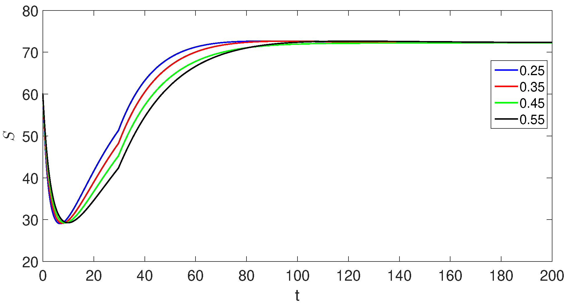
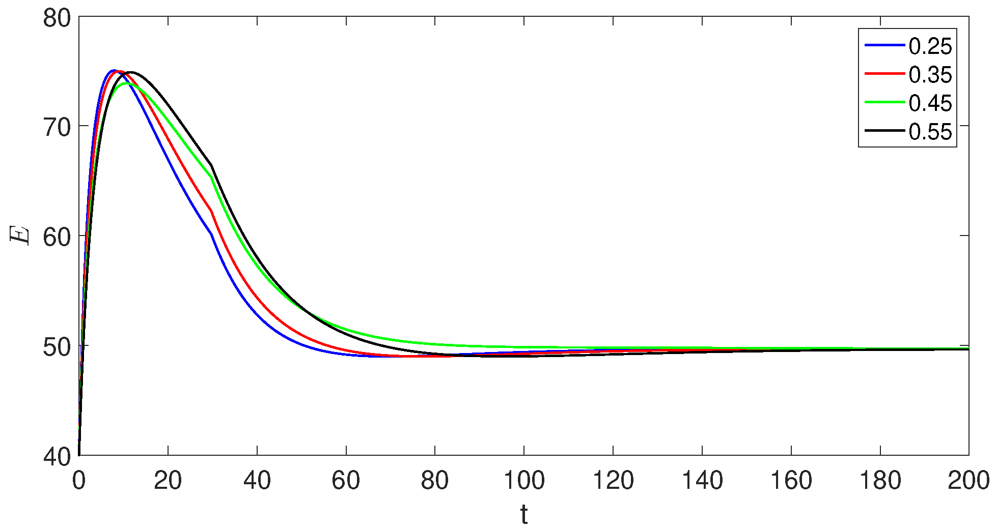
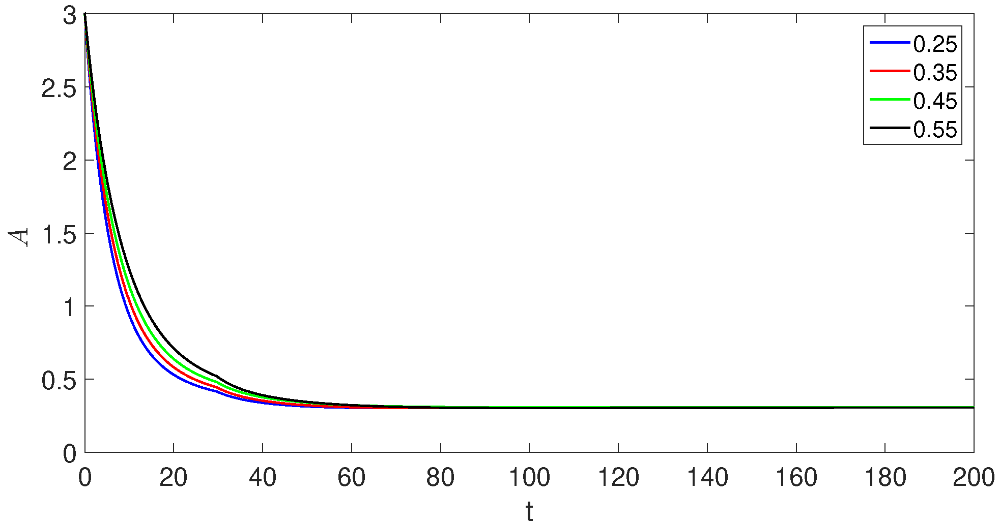
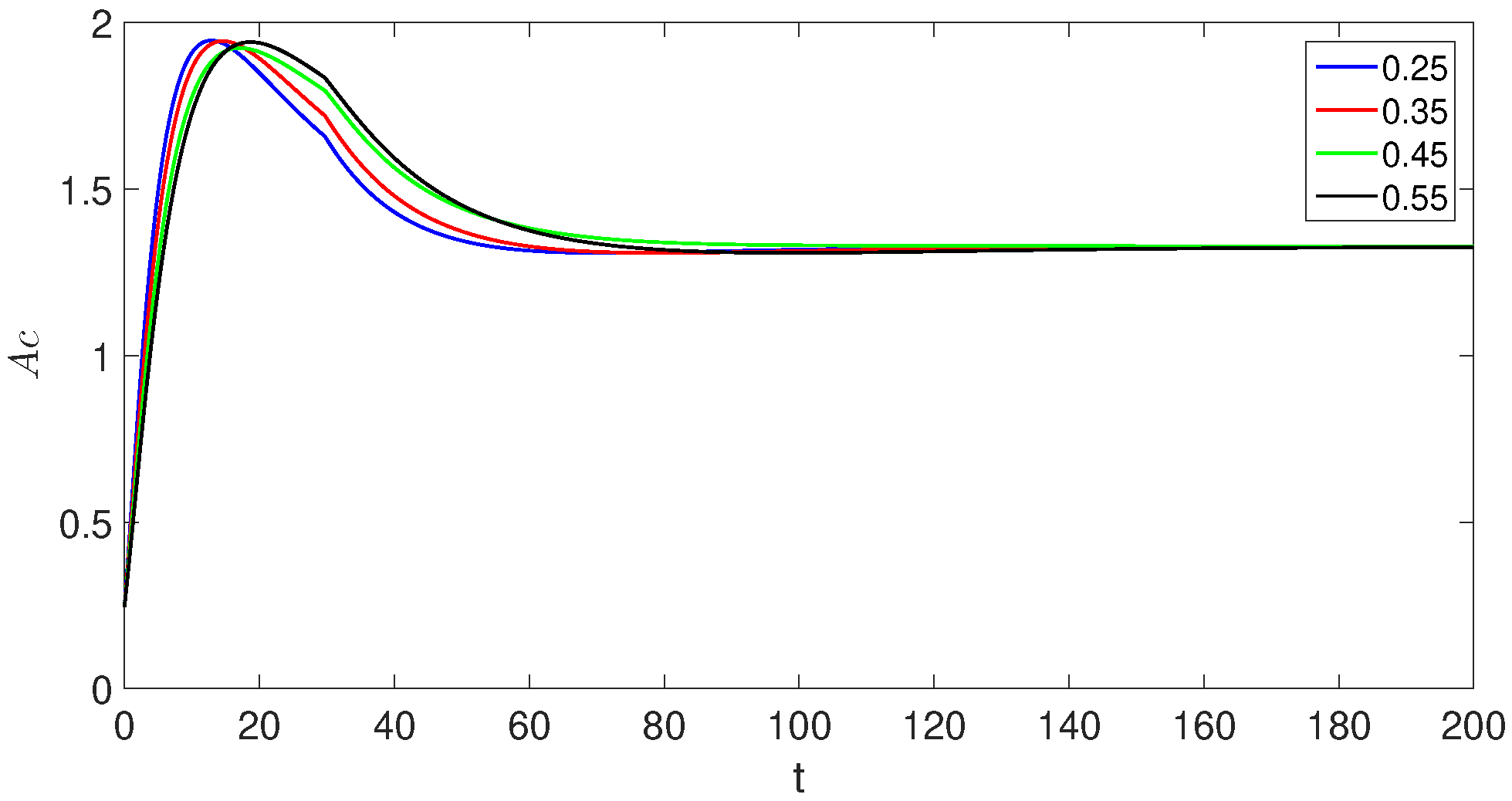
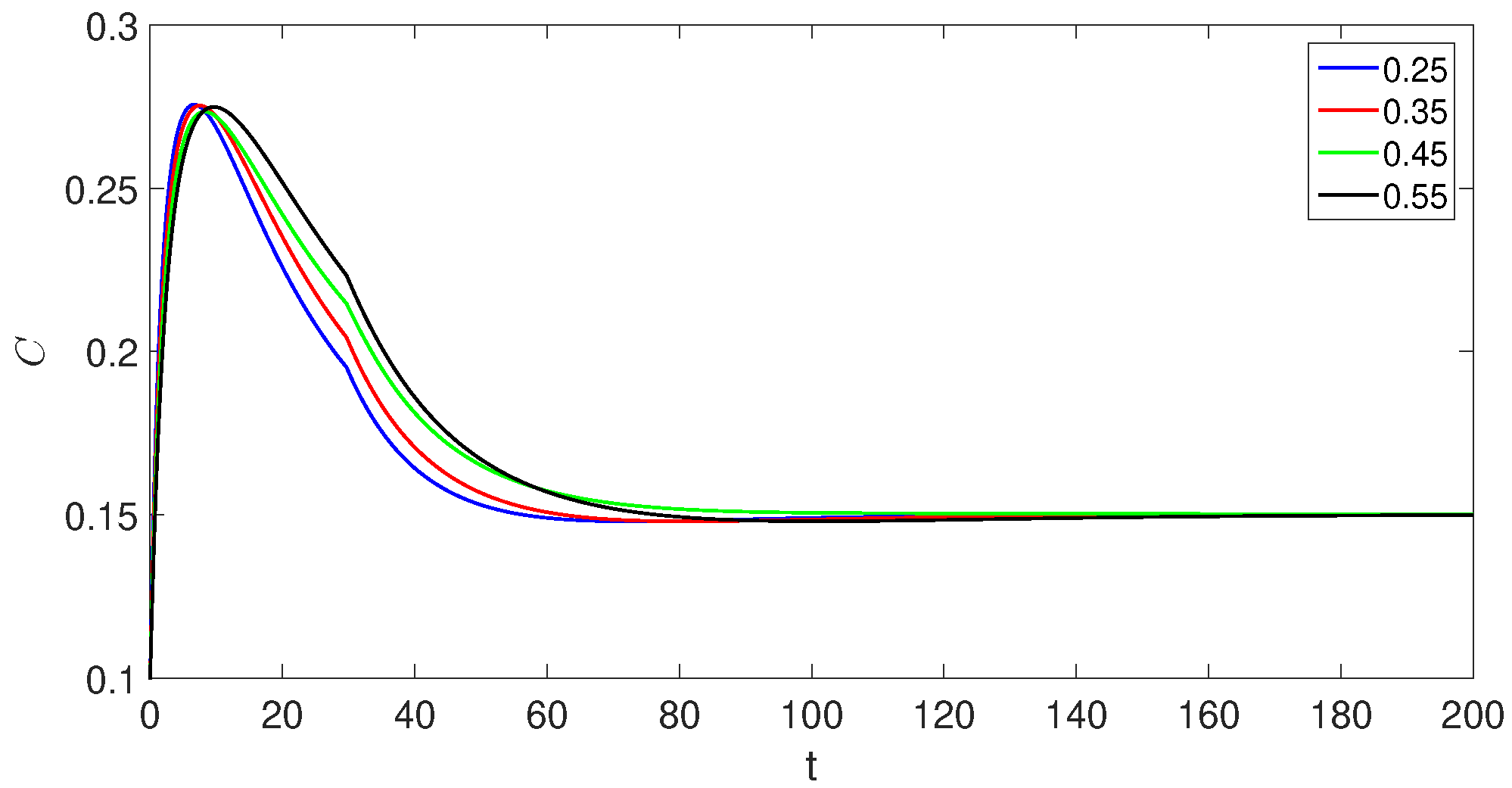
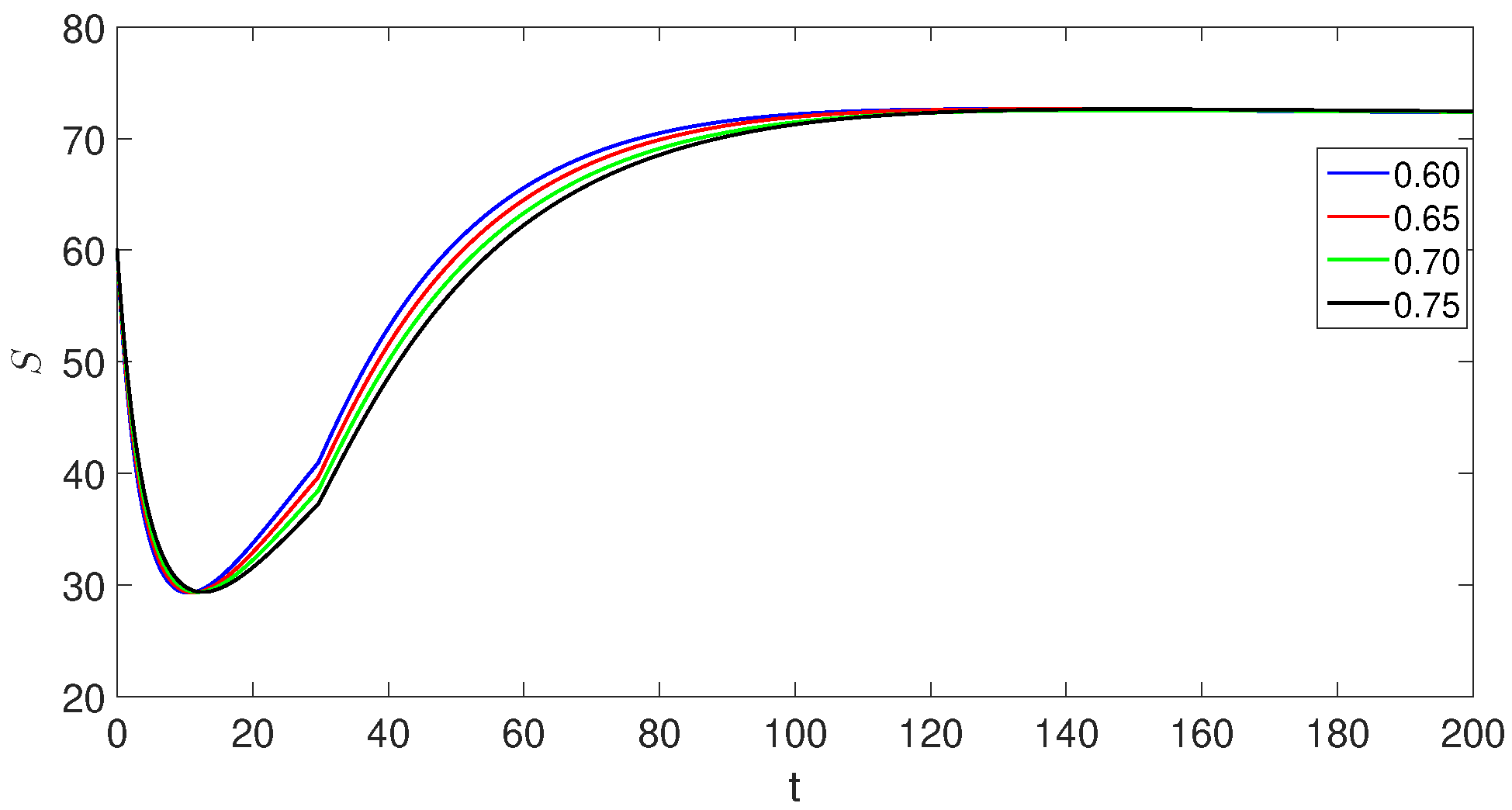
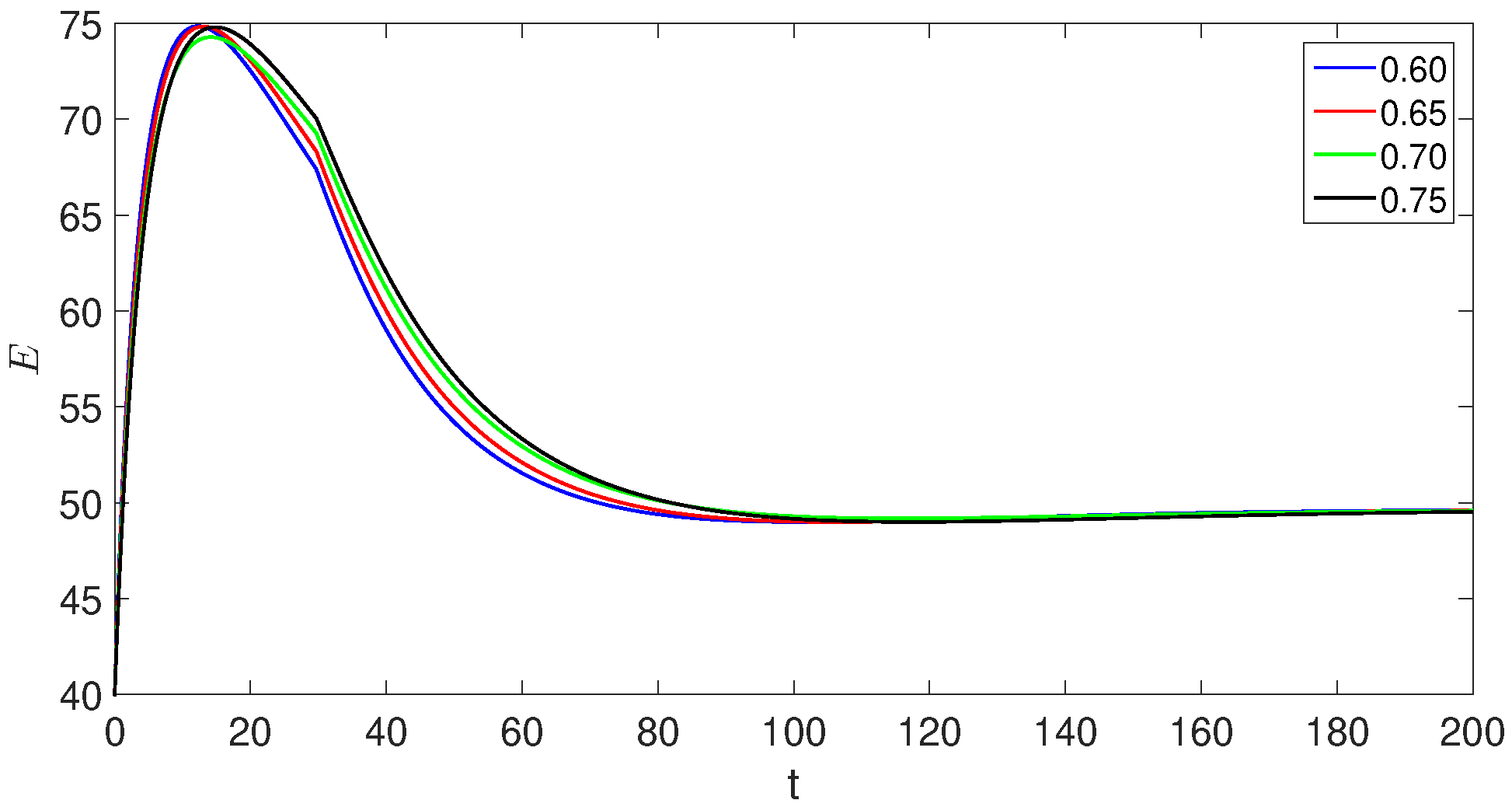
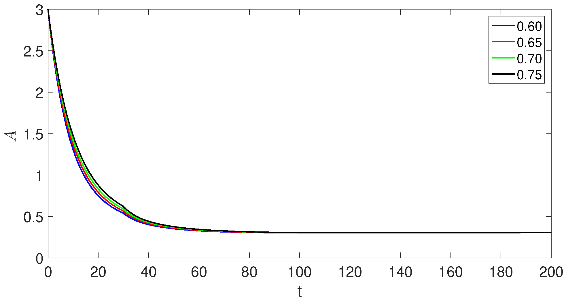
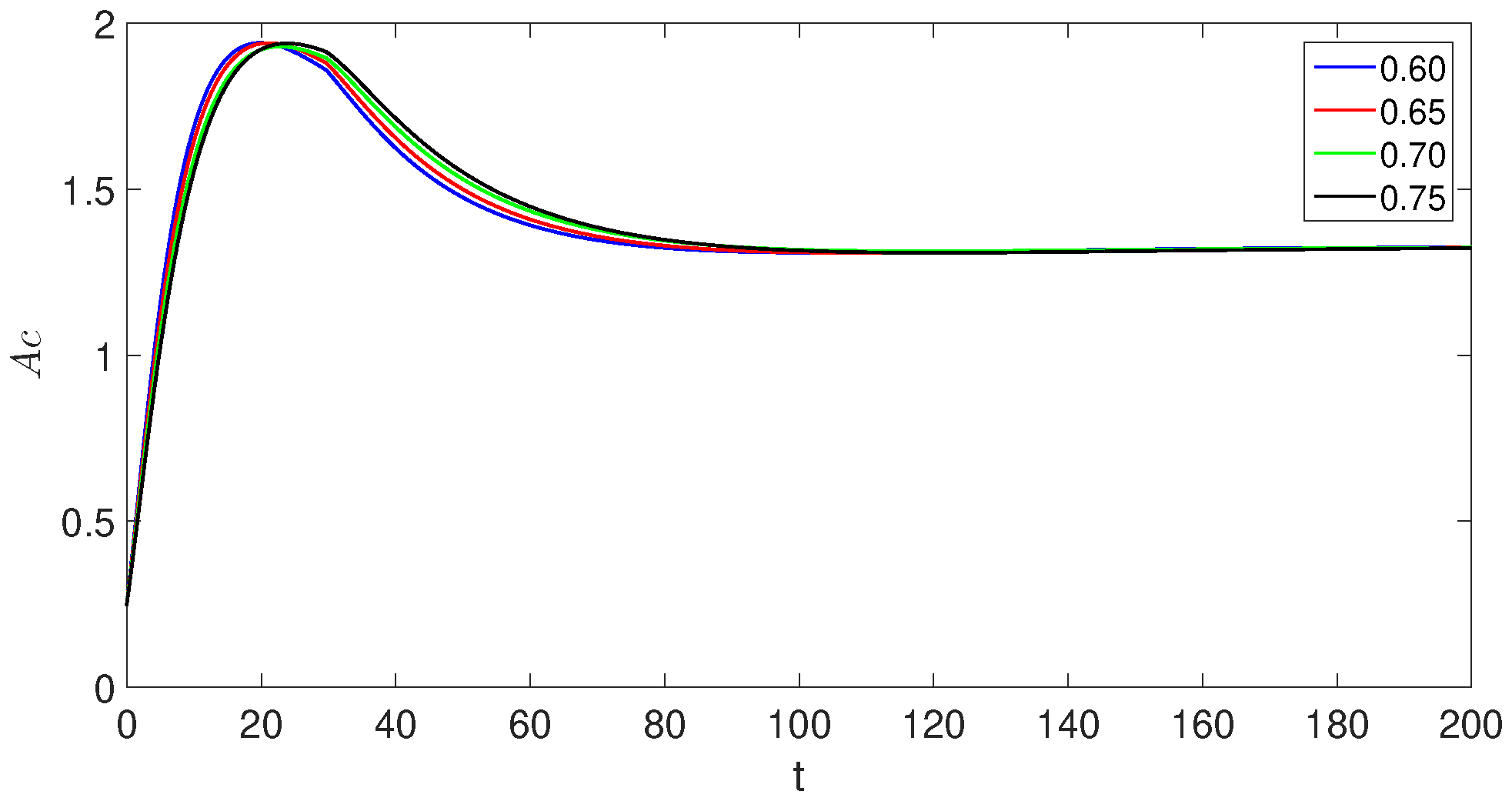
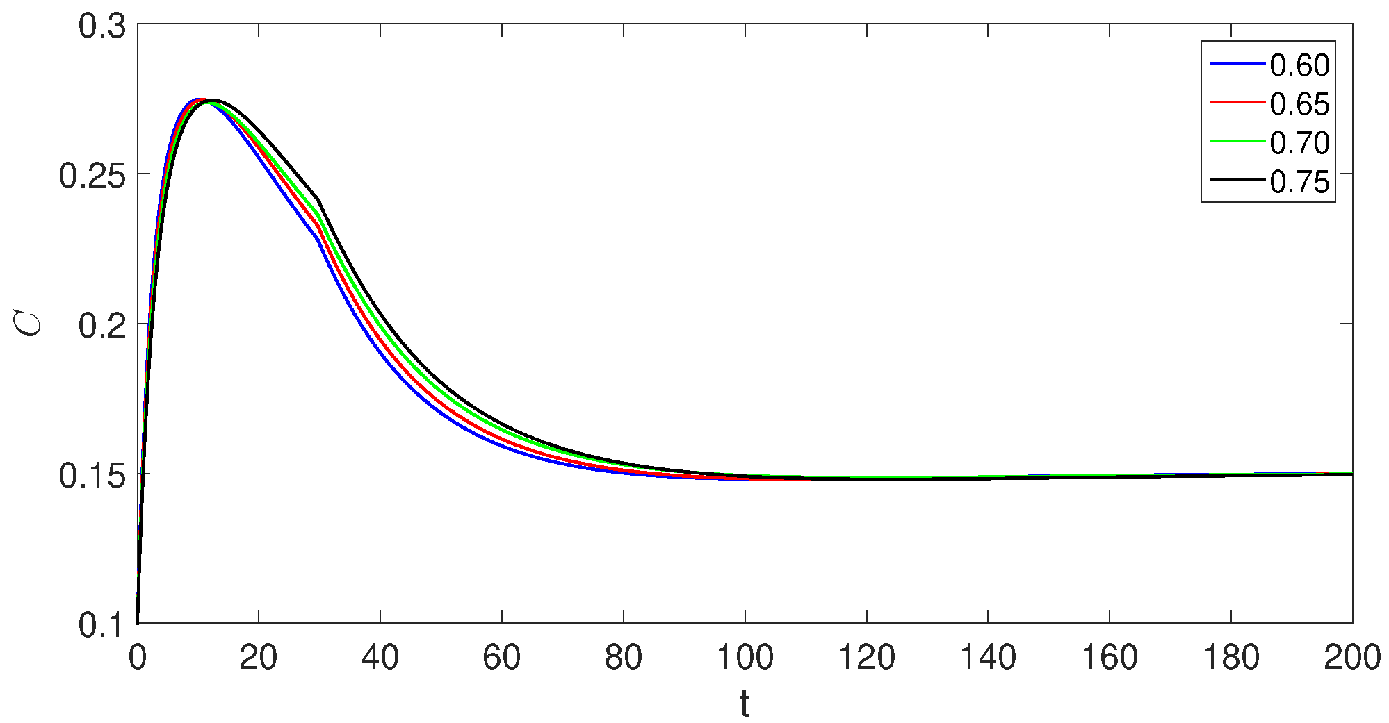
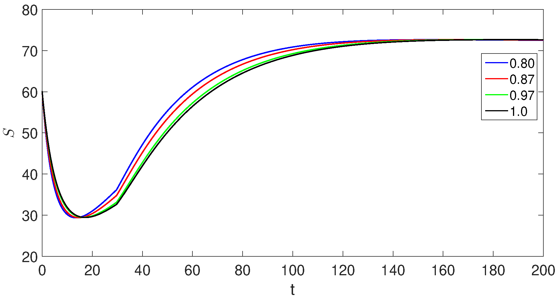
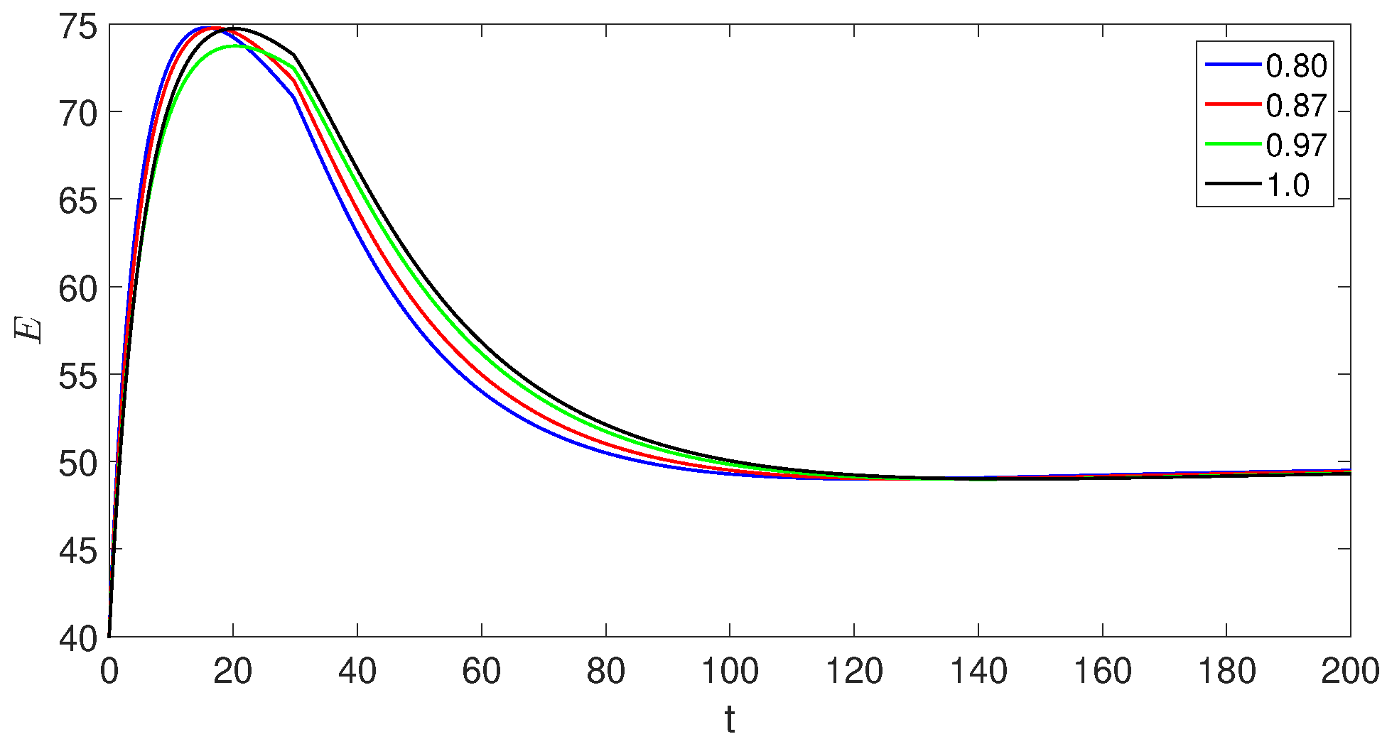
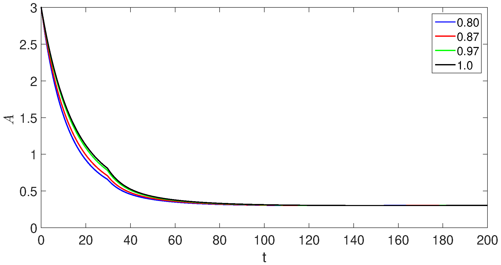
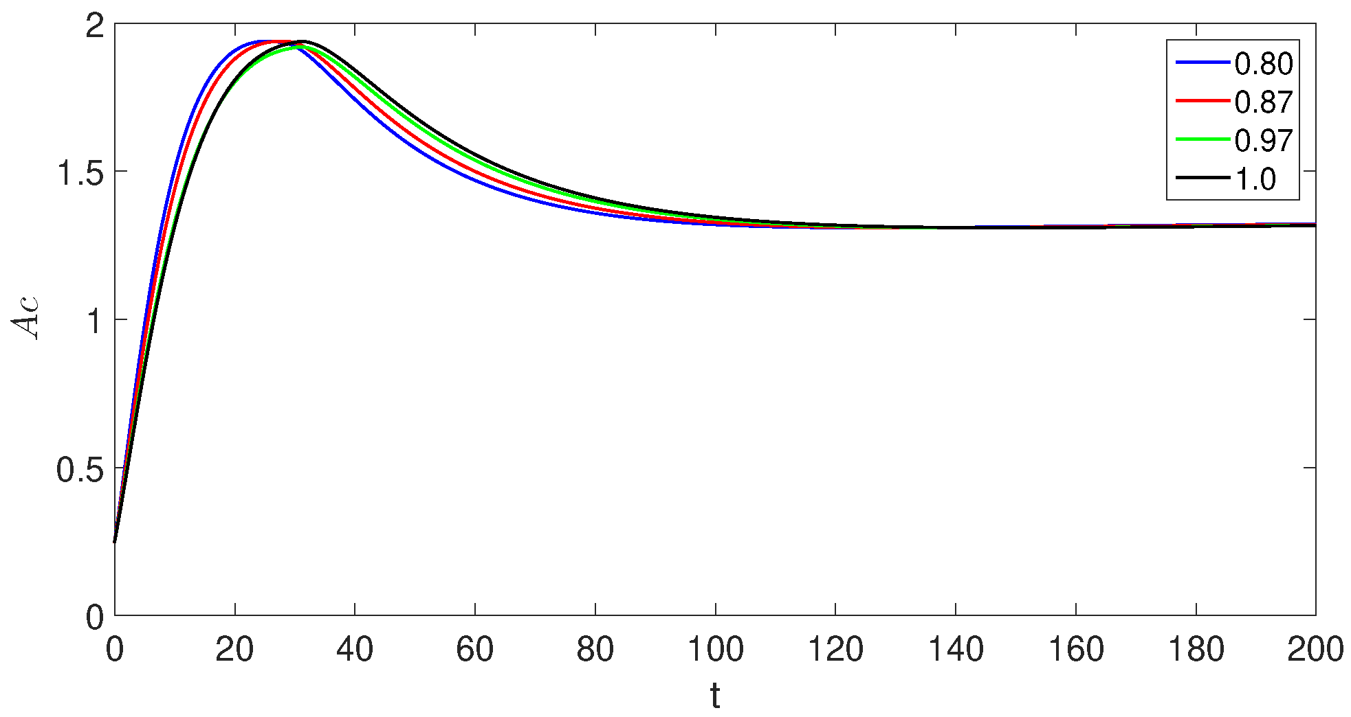
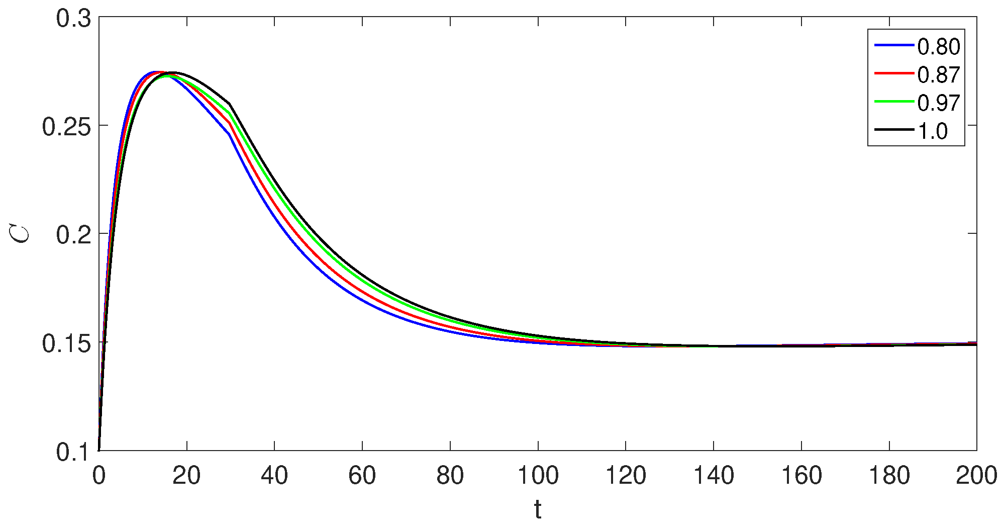
  • The crossover behaviors in each compartment due to the piecewise version of derivatives near the point t 1 < 100 ;
  • The decreases and increases over time in susceptible class, exposed classes, and the concerned changes in other compartments A ,   A c ,   C can be observed easily;
  • Figure 1 displays the sensitivity indices of parameters in the HBV model. From the sensitivity indices in Figure 1, we note that the birth rate of susceptible individuals, the effective contact rate, and the death rate due to acute disease have the most significant impact on the model’s behavior;
  • The population of the exposed, asymptomatic carrier, and chronic infected individuals model classes increases and reaches its peak value around ι = 20 , but in the second sub-interval, they start decreasing.

8. Conclusions

We have studied a dynamics system of HBV with the class of asymptomatic carriers with some new perspectives of fractional calculus. We have used piecewise derivatives of fractional orders with non-local kernel as well as singular kernel. We studied fundamental characteristics of the HBV model (5), such as the identification of an invariant region, positivity of solutions, equilibrium and endemic points, basic reproduction number, local and global Stability, and sensitivity indices. Also, we have established some appropriate conditions for the existence of such models using the tools of nonlinear analysis. In addition, for numerical illustration, we have used Adam Bashforth’s numerical method. Using the real values of parameters already reported, the concerned results have been presented graphically under various fractional orders. The model numerically demonstrated the crossover effect in the dynamics using the time domain for transmission [ 0 ,   200 ] near the point where t 1 < 100 . The mentioned aspects of fractional calculus have recently been recognized as a powerful tool to elaborate the sudden or abrupt changes in real-world phenomena in more brilliant ways. Age-specific data reveals that acute HBV infection is typically asymptomatic in infants, young children (under the age of 10), and immunocompromised adults. Symptomatic cases are more common among adults and older children, accounting for approximately 30 to 50% of infections. Infected individuals with HBV without symptoms can transmit the virus and may face the risk of liver damage or even death, particularly if they remain asymptomatic for over six months. In the future, we will use these methodologies in other complex dynamical models of other diseases.

Author Contributions

Conceptualization: K.A.A., M.A.A. and K.S.; Formal analysis: K.A.A., M.A.A. and K.S.; Investigation: K.A.A., M.A.A. and K.S.; Methodology: K.A.A., M.A.A. and K.S.; Writing—original draft: K.A.A., M.A.A. and K.S. All authors have read and agreed to the published version of the manuscript.

Funding

This research received no external funding.

Data Availability Statement

The authors declare that all data and materials in this paper are available and veritable.

Acknowledgments

The researchers wish to extend their sincere gratitude to the Deanship of Scientific Research at the Islamic University of Madinah for the support provided to the Post-Publishing Program.

Conflicts of Interest

The authors declare that they have no known competing financial interests or personal relationships that could have appeared to influence the work reported in this paper.

References

  1. World Health Organization (WHO) Media Centre. Available online: http://www.who.int/mediacentre/factsheets/fs204/en/ (accessed on 12 February 2018).
  2. Thornley, S.; Bullen, C.; Roberts, M. Hepatitis B in a high prevalence New Zealand population: A mathematical model applied to infection control policy. J. Theor. Biol. 2008, 254, 599–603. [Google Scholar] [CrossRef] [PubMed]
  3. Mann, J.; Roberts, M. Modelling the epidemiology of hepatitis B in New Zealand. J. Theoret. Biol. 2011, 269, 266–272. [Google Scholar] [CrossRef] [PubMed]
  4. Wang, J.; Pang, J.; Liu, X. Modelling diseases with relapse and nonlinear incidence of infection: A multi-group epidemic model. J. Biolog. Dyn. 2014, 8, 99–116. [Google Scholar] [CrossRef] [PubMed]
  5. Zhao, S.; Xu, Z.; Lu, Y. A mathematical model of hepatitis B virus transmission and its application for vaccination strategy in China. Int. J. Epidemiol. 2000, 29, 744–752. [Google Scholar] [CrossRef] [PubMed]
  6. Wang, K.; Wang, W.; Song, S. Dynamics of an HBV model with diffusion and delay. J. Theor. Biol. 2008, 253, 36–44. [Google Scholar] [CrossRef] [PubMed]
  7. Xu, R.; Ma, Z. An HBV model with diffusion and time delay. J. Theor. Biol. 2009, 257, 499–509. [Google Scholar] [CrossRef] [PubMed]
  8. Kilbas, A.A.; Shrivastava, H.M.; Trujillo, J.J. Theory and Applications of Fractional Differential Equations; Elsevier: Amsterdam, The Netherlands, 2006. [Google Scholar]
  9. Podlubny, I. Fractional Differential Equations; Academic Press: San Diego, CA, USA, 1999. [Google Scholar]
  10. Atangana, A.; Baleanu, D. New fractional derivatives with non-local and non-singular kernel: Theory and application to heat transfer model. Therm. Sci. 2016, 20, 763–769. [Google Scholar] [CrossRef]
  11. Atangana, A.; Araz, S.I. Nonlinear equations with global differential and integral operators: Existence, uniqueness with application to epidemiology. Results Phys. 2020, 20, 103593. [Google Scholar] [CrossRef]
  12. Khan, H.; Alam, K.; Gulzar, H.; Etemad, S.; Rezapour, S. A case study of fractal-fractional tuberculosis model in China: Existence and stability theories along with numerical simulations. Math. And Computers Simul. 2022, 198, 455–473. [Google Scholar] [CrossRef]
  13. Khan, A.; Gómez-Aguilar, J.F.; Khan, T.S.; Khan, H. Stability analysis and numerical solutions of fractional order HIV/AIDS model. Chaos Solitons Fractals 2019, 122, 119–128. [Google Scholar] [CrossRef]
  14. Alkahtani, B.S.T. Chua’s circuit model with Atangana-Baleanu derivative with fractional order. Chaos Solitons Fractals 2016, 89, 547–551. [Google Scholar] [CrossRef]
  15. Almalahi, M.A.; Panchal, S.K.; Shatanawi, W.; Abdo, M.S.; Shah, K.; Abodayeh, K. Analytical study of transmission dynamics of 2019-nCoV pandemic via fractal fractional operator. Results Phys. 2021, 24, 104045. [Google Scholar] [CrossRef]
  16. Abdeljawad, T. A Lyapunov type inequality for fractional operators with nonsingular Mittag-Leffler kernel. J. Inequal. Appl. 2017, 2017, 130. [Google Scholar] [CrossRef] [PubMed]
  17. Abdeljawad, T.; Baleanu, D. On fractional derivatives with generalized Mittag-Leffler kernels. Adv. Differ. Equ. 2018, 2018, 468. [Google Scholar] [CrossRef]
  18. Abdeljawad, T. Fractional operators with generalized Mittag-Leffler kernels and their differintegrals. Chaos 2019, 29, 023102. [Google Scholar] [CrossRef] [PubMed]
  19. Atangana, A.; Araz, S.I. New concept in calculus: Piecewise differential and integral operators. Chaos Solitons Fractals 2021, 145, 110638. [Google Scholar] [CrossRef]
  20. Gul, N.; Bilal, R.; Algehyne, E.A.; Alshehri, M.G.; Khan, M.A.; Chu, Y.M.; Islam, S. The dynamics of fractional order Hepatitis B virus model with asymptomatic carriers. Alex. Eng. J. 2021, 60, 3945–3955. [Google Scholar] [CrossRef]
  21. Kumar, S.; Chauhan, R.P.; Aly, A.A.; Momani, S.; Hadid, S. A study on fractional HBV model through singular and non-singular derivatives. Eur. Phys. J. Spec. Top. 2022, 231, 1885–1904. [Google Scholar] [CrossRef]
  22. Shah, S.A.A.; Khan, M.A.; Farooq, M.; Ullah, S.; Alzahrani, E.O. A fractional order model for Hepatitis B virus with treatment via Atangana–Baleanu derivative. Phys. Stat. Mech. Its Appl. 2020, 538, 122636. [Google Scholar] [CrossRef]
  23. Alazman, I.; Alkahtani, B.S.T. Investigation of Novel Piecewise Fractional Mathematical Model for COVID-19. Fractal Fract. 2022, 6, 661. [Google Scholar] [CrossRef]
  24. Momani, S.; Abu Arqub, O.; Maayah, B. Piecewise optimal fractional reproducing kernel solution and convergence analysis for the Atangana-Baleanu-Caputo model of the Lienarders equation. Fractals 2020, 28, 2040007. [Google Scholar] [CrossRef]
  25. Alkahtani, B.S.T. Dynamical Analysis of Rubella Disease Model in the Context of Fractional Piecewise Derivative: Simulations with Real Statistical Data. Fractal Fract. 2023, 7, 746. [Google Scholar] [CrossRef]
  26. Kattan, D.A.; Hammad, H.A. Existence and Stability Results for Piecewise Caputo-Fabrizio Fractional Differential Equations with Mixed Delays. Fractal Fract. 2023, 7, 644. [Google Scholar] [CrossRef]
  27. Van den Driessche, P.; Watmough, J. Reproduction numbers and sub-threshold endemic equilibria for compartmental models of disease transmission. Math. Biosci. 2002, 180, 29–48. [Google Scholar] [CrossRef]
  28. Alkahtani, B.S.T.; Atangana, A.; Koca, I. Novel analysis of the fractional Zika model using the Adams type predictor-corrector rule for non-singular and non-local fractional operators. J. Nonlinear Sci. Appl. 2017, 10, 3191–3200. [Google Scholar] [CrossRef]
  29. Garrappa, R. Numerical solution of fractional differential equations: A survey and a software tutorial. Mathematics 2018, 6, 16. [Google Scholar] [CrossRef]
  30. Zabidi, N.A.; Abdul Majid, Z.; Kilicman, A.; Rabiei, F. Numerical solutions of fractional differential equations by using fractional explicit Adams method. Mathematics 2020, 8, 1675. [Google Scholar] [CrossRef]
Figure 1. Presentation of sensitivity indices involved in the computation of R 0 .
Fractalfract 07 00844 g001
Figure 2. Graphical presentations of susceptible individuals for the HBV using the given fractional orders.
Fractalfract 07 00844 g002
Figure 3. Graphical presentations of the exposed population for the HBV using the given fractional orders.
Fractalfract 07 00844 g003
Figure 4. Graphical presentations of the acutely infected population for HBV using the given fractional orders.
Fractalfract 07 00844 g004
Figure 5. Graphical presentations of approximate solutions of asymptomatic carrier for the proposed model using the given fractional orders.
Fractalfract 07 00844 g005
Figure 6. Graphical presentations of approximate solutions of chronic infected individuals for the proposed model using the given fractional orders.
Fractalfract 07 00844 g006
Figure 7. Graphical presentations of susceptible individuals for the HBV using the given fractional orders.
Fractalfract 07 00844 g007
Figure 8. Graphical presentations of the exposed population for the HBV using the given fractional orders.
Fractalfract 07 00844 g008
Figure 9. Graphical presentations of the acutely infected population for HBV using the given fractional orders.
Fractalfract 07 00844 g009
Figure 10. Graphical presentations of approximate solutions of asymptomatic carrier for the proposed model using the given fractional orders.
Fractalfract 07 00844 g010
Figure 11. Graphical presentations of approximate solutions of C for the proposed model using the given fractional orders.
Fractalfract 07 00844 g011
Figure 12. Graphical presentations of approximate solutions of S for the proposed model using the given fractional orders.
Fractalfract 07 00844 g012
Figure 13. Graphical presentations of approximate solutions of E for the proposed model using the given fractional orders.
Fractalfract 07 00844 g013
Figure 14. Graphical presentations of approximate solutions of A for the proposed model using the given fractional orders.
Fractalfract 07 00844 g014
Figure 15. Graphical presentations of approximate solutions of A c for the proposed model using the given fractional orders.
Fractalfract 07 00844 g015
Figure 16. Graphical presentations of approximate solutions of chronic infected individuals for the proposed model using the given fractional orders.
Fractalfract 07 00844 g016
Disclaimer/Publisher’s Note: The statements, opinions and data contained in all publications are solely those of the individual author(s) and contributor(s) and not of MDPI and/or the editor(s). MDPI and/or the editor(s) disclaim responsibility for any injury to people or property resulting from any ideas, methods, instructions or products referred to in the content.

