


Fractional-Order Accumulative Generation with Discrete Convolution Transformation

Department of Mathematics, Communication University of China, Beijing 100024, China
Fractal Fract. 2023, 7(5), 402; https://doi.org/10.3390/fractalfract7050402
Submission received: 2 April 2023
/
Revised: 6 May 2023
/
Accepted: 12 May 2023
/
Published: 16 May 2023
(This article belongs to the Special Issue Fractional-Order Circuits, Systems, and Signal Processing)
Abstract
:A new fractional accumulation technique based on discrete sequence convolution transform was developed. The accumulation system, whose unit impulse response is the accumulation convolution sequence, was constructed; then, the order was extended to fractional orders. The fractional accumulative convolution grey forecasting model GM was established on the sequence convolution. From the viewpoint of sequence convolution, we can better understand the mechanism of accumulative generation. Real cases were used to verify the validity and effectiveness of the fractional accumulative convolution method.
1. Introduction
Due to the finite cognitive competence of human beings, the information obtained from the investigated system is always incomplete and inaccurate. The incompleteness and inaccuracy of information are absolute, while completeness and accuracy are relative [1]. Prof. Julong Deng proposed the grey system theory to solve undetermined problems, in which the given information is lacking and the data for modelling are few.
In contrast to traditional statistical models, such as the Bayesian approach [2], maximum likelihood estimation [3], modern artificial neural network [4], and machine learning methods [5], which usually need many samples, the grey model requires less data modelling [1]. It makes full use of the limited data from a small sample and excavates more useful information from the data. In the early stage, Deng pointed out that only four data points were sufficient for GM modelling [6]. Yao et al. put forward the mathematical proof indicating that small samples have greater accuracy than large samples [7]. Matrix perturbation theory was introduced to analyse the grey model, suitable for modelling small samples, by Wu, and Xu et al. [8,9]. Wang applied the grey power model to simulate small oscillating samples [10]. Talafuse modelled a small sample on discrete reliability growth with the grey model and achieved more accurate predictions than the traditional parametric and non-parametric methods [11]. Ma proposed KGM combined with kernel learning to model the non-linearity of multi-input and single-output sequences and proved it to be more stable and efficient than the machine learning models, such as least squares support vector machines [12]. The grey model has been applied with high efficiency in modelling small data samples in science and engineering technologies [13], energy resources [14], traffic control [15], health care [16], economics [17], management [18], ecology [19], agriculture [20], etc., and has achieved significant economic and social benefits [21,22,23,24].
The grey model employs a kind of sequence operator called accumulative generation operator to act on the system behaviour sequence to provide intermediate data for the grey model [25], distinguishing itself from other forecasting models that directly model the original data series. The acting of the accumulative generation operator on the original data sequence removes random fluctuation in the data, and the acted-upon sequence approximates to the quasi-exponential law. Many systems in economics, ecosystems, etc., are general energy systems, and energy transfer follows the power law, which is the foundation of grey modelling [26]. Prof. Sifeng Liu proposed the concept of the grey sequence operator [27] and then considered the accumulative generation procedure as the action of the sequence operator called the accumulative generation operator (AGO) [26]. The AGO can make the data sequence follow the power law, but the over-acting of the AGO can also destroy the power law [21].
In nature, there are many systems with non-integral-order derivative effects; the fractional-order derivative is a better way to describe this kind of system behaviour than ordinary integral-order models. With the concept of “in between”, the fractional-order derivative is the general extension of the normal integral-order derivative, applied in many disciplines, such as fractional system analysis and control [28,29,30], energy resource modelling and prediction [31,32], air pollution and environment protection [33,34], etc.
A higher-order operator is a natural concept indicating the repeated action of the operator on the data sequence, i.e., the AGO acting m times on the data sequence leads to the m-th-order AGO, where m is a positive integer [22]. Wu et al. considered the accumulative generation operator a square matrix; then, the action of AGOs of different orders was the same as the power of the square matrix [35]. From this viewpoint, the explicit expression of the positive integral m-th-order AGO was derived; then, it could be very quickly extended to fractional orders, i.e., the fractional-order accumulative operator (FAO), establishing the fractional-order grey forecasting model (FGM) [35,36,37,38]. Due to great improvement in forecasting precision, FAO and FGM have attracted a lot of attention and have become hot topics in recent years. Xiao, and Mao et al. used matrix analysis to explore the modelling mechanism and theoretical significance of fractional accumulation grey models [39,40]. Soon, the order was extended to arbitrary real numbers by Meng, and Zeng et al. [41,42,43]. Recently, Wu et al. unified the expression of AGOs; then, they extended the order numbers to the widest field, i.e., the complex number order [44].
Although the AGO has been discussed for a long time and has been widely used in many fields, little attention has been paid to its essence and mechanism. Wei, and Xie et al. introduced the integral matching method to explain that the AGO is a discrete form of the integral of the continuous function approximated by a piecewise constant in each subinterval, and due to the approximated discrete form of the integral being cumulative summation, the operator gained a new name, cumulative sum operator [45,46,47]. Chen used convolution transformation to improve the accumulative generation procedure and pointed out that convolution transformation could enhance the smoothness of the data sequence, which could be used in grey modelling [48]. Lin et al. quantitatively studied the mechanism and power of the AGO by applying spectrum analysis in the frequency domain [49,50,51,52].
The paper proposes fractional accumulation with the discrete convolution transform of finite sequences and aims to interpret its physical meaning from the perspective of signal processing. The main contributions are listed as follows:
- (1)
- The concept of discrete convolution transform is introduced in accumulative generation. In fact, the unit impulse response of the accumulative generation system is found and is named accumulative generation convolution sequence. This is the discretization of the AGO in the time domain.
- (2)
- By extending the concept in (1) to the fractional-order accumulative generation convolution sequence, the unit impulse response of the fractional-order accumulative generation system is obtained. In fact, the discrete form of the fractional accumulation operator (FAO) in the time domain is explicitly represented, which makes the physical meaning of the FAO self-evident.
- (3)
- The fractional-order accumulative generation convolution transform and its inversion are mutually inverse. They do not impose any extra error on data transformation. The inversion of the fractional-order accumulative generation convolution sequence can be calculated directly by assigning the minus fractional order, without demanding a round number order (compare with [8] (p. 1780)).
- (4)
- According to model fitting error, the fractional accumulation grey model can dynamically adjust the order to model and predict the system behaviour data better.
Convolution transformation is a powerful tool in digital signal process [53]. In this framework, a new viewpoint to understand the mechanism of AGO emerges. An AGO can be understood as a linear time invariant system. Convolving an input sequence with the unit impulse responsesequence yields an accumulated output sequence [54].
The remainder of the paper is organized as follows. The integral-order accumulative convolution sequence is introduced and extended to arbitrary real numbers in Section 2. The fractional accumulative convolution grey model is discussed in Section 3. Some real cases are used to demonstrate the validity of the fractional accumulative convolution transform in Section 4. Finally, Section 5 discusses the conclusions.
2. The Accumulative Generation with Discrete Convolution Transform
In this section, we start from the classical definition of the AGO, then introduce the finite sequence convolution and construct the accumulative convolution sequence to fulfil the accumulative generation procedure and the extend the accumulative convolution sequenceto the integral- and fractional-order.
Definition 1.
The accumulative generation operator (AGO) for a sequence is as follows [25]
Here, is a sequence with length N with the integral-index n varying from 0 to and is one datum in the sequence. The superscript represents the order of accumulation, e.g., is the zeroth-order accumulated sequence, i.e., the original sequence; while represents the first-order accumulated sequence.
Applying the AGO m times leads to the integral-order accumulated sequence [21,26]
where (set of natural numbers).
Definition 2.
Given two sequences with length N, and , then their discrete convolution is [54]
By Definition 2, the discrete convolution operation is commutative.
Definition 3.
Set to be the unit impulse sequence on the non-negative part of the time axis, i.e., [55]
By Definitions 2 and 3, the invariance of the unit impulse sequence in the convolution operation is obtained, i.e., does not change anything and is identically equal to . Therefore, in the convolution operation, is an identity element. Moreover, for a positive integer m,
Definition 4.
Set and to be two sequences. If their convolution yields to the unit impulse sequence, then they are mutually inverse, denoted by .
Based on the above definitions, we arrived at Theorem (1) to represent the AGO in the form of finite sequence convolution. Since the classical accumulative generation operator is denoted in uppercase, the accumulative convolution sequence is denoted by in lowercase for distinction.
Theorem 1.
For a sequence , denote the first-order accumulated sequence obtained by the AGO in (1) as . Then it can be regenerated by convolution
The is called the accumulative convolution sequence, and is represented by
Proof.
From Definition 2 and Equation (5),
which concludes the result. □
Remark 1.
The acts on a sequence, denoted with a pair of round brackets, i.e., , which yields to the ; while the accumulative convolution sequence is a data sequence by itself, in which a pair of square brackets indicates that is a datum. Convolution transforming the original sequence by the accumulative convolution sequence also generates the first-order accumulated sequence, i.e., , which plays the same role of the AGO. To avoid confusion, the same name but in lower case “ago” denotes the accumulative convolution sequence. Simply, is an operator; while is a datum from an accumulative convolution sequence. They are fundamentally different.
Definition 5.
The convolution power is defined by a sequence convolving with itself for k times, where k is a positive integer,
For completeness of Definition 5 , the zeroth convolution power is set to be the identity element, i.e.,
By (5),
Comparing (7) and (10), the accumulative convolution sequence can be represented by summation of the first n terms of the convolution power series
Convolving with (11) yields the unit impulse sequence, i.e.,
According to Definition 4, is the inverse accumulative convolution sequence of . It is denoted by .
Based on (12), the first-order accumulative convolution sequence is extended to the integral-order, i.e., , with (set of positive integers),
This leads to the definition of the positive integral-order accumulative convolution sequence. Using Newton’s generalized binomial theorem and the unit impulse sequence in Definition 3,
where is the extended combination number, given by
According to (4) and (10), the m-th power of the accumulative convolution sequence yields
For , (16) is always equal to 1, i.e., . For , by (4), the unit impulse is equal to zero when , thus
Therefore, the positive-integral m-th power of the accumulative convolution sequence is
For the negative-integral -th-order accumulative convolution sequence,
For , (18) is also equal to 1, i.e., . For ,
If , k can reach n and if and only if . Thus,
Otherwise, if , k is also less than n, which causes the unit impulse to equal zero. Thus
Therefore, the negative-integral -th power of the accumulative convolution sequence is
According to Equations (17) and (19), the following theorem unifies the integral m-th-order accumulative convolution sequence.
Theorem 2.
Let be the accumulative convolution sequence, then the integral m-th-order accumulative convolution sequence with (set of integers) is unified, i.e.,
Next, the order of accumulative convolution sequence is extended to fractional orders. Based on (13), for a positive real number (set of positive real numbers),
Thus, the r-th power of the accumulative convolution sequence is
Using Newton’s generalized binomial theorem and the definition of in (4),
Similarly, (22) is always equal to 1 when , i.e., . For ,
Therefore, the positive real r-th power of the accumulative convolution sequence is
For the negative real -th-order accumulative convolution sequence,
Using Newton’s generalized binomial theorem again,
By the definition of unit impulse in (4),
Thus, (24) is always equal to 1 for , i.e., . For ,
Therefore, (24) becomes
According to Equations (23) and (25), a unified expression of the real number r-th-order accumulative convolution sequence is obtained in the following theorem.
Theorem 3.
Let be the accumulative convolution sequence, then the real r-th-order accumulative convolution sequence with (set of real numbers) is unified, i.e.,
3. Grey Forecasting Model with Fractional Accumulative Convolution
The fractional accumulative convolution is introduced into GM in this section, leading to a new grey model.
For a given sequence and the accumulation order r, according to Definition 2 and the Theorem 3, the accumulated sequence can be represented by the convolution transform with the r-th-order accumulative convolution sequence .
Definition 6.
Givenan original sequence , and a real number r-th-order accumulative convolution sequence defined in (26), their discrete convolution yields the r-th-order accumulated sequence , i.e.,
Suppose be the equidistant sampling sequence from a differentiable function , satisfying the first-order ordinary differential equation
For a given sequence , the coefficients and in (28) are determined. Both sides of (28) are integrated on subinterval ,
By the trapezoidal rule, a discrete form of (28) is obtained,
Remark 2.
Equation (30) is the so-called fractional r-th-order accumulative convolution grey model, denoting GM with . The superscript represents the accumulative convolution sequence with order r. When , it turns out to be the GM .
For , (30) leads to a linear system
where
Linear system (31) contains equations, but there are only two unknowns, and . It is an over-determined system when . Therefore, the solution of (31) in the sense of least squares is equivalent to the solution of the normal equation
and the unknown coefficients can be estimated by
The ODE (28) can be solved by
Then the time response of GM can be achieved by substituting coefficients obtained from (33) into (34)
The timeresponse sequence from (35) can be convolved with the corresponding inverse -th-order accumulative convolution sequence to obtain the estimated data sequence, i.e.,
The mean absolute percentage error (MAPE) is employed here to indicate errors between the estimated data and original data , i.e.,
Finally, the modelling procedure for the fractional-order accumulative convolution GM model is described in Algorithm 1, and depends on Algorithm 2 for finite sequence convolution based on Definition 2 and Algorithm 3 for the fractional accumulative convolution sequence based on Theorem 3.
| Algorithm 1 Fractional-order accumulative convolution GM model |
| Algorithm 2 Finite sequence convolution |
|
| Algorithm 3 Fractional-order accumulative convolution sequence |
|
4. Cases Study
Case 1
Case 2
(Inverse fractional accumulative convolution sequence). Set , generate the inverse -th-order accumulative convolution sequence with different orders , , , , , , , . The inverse fractional -th-order accumulative convolution sequences are generated by Algorithm 3, and displayed in Table 2 and Figure 2.
Case 3
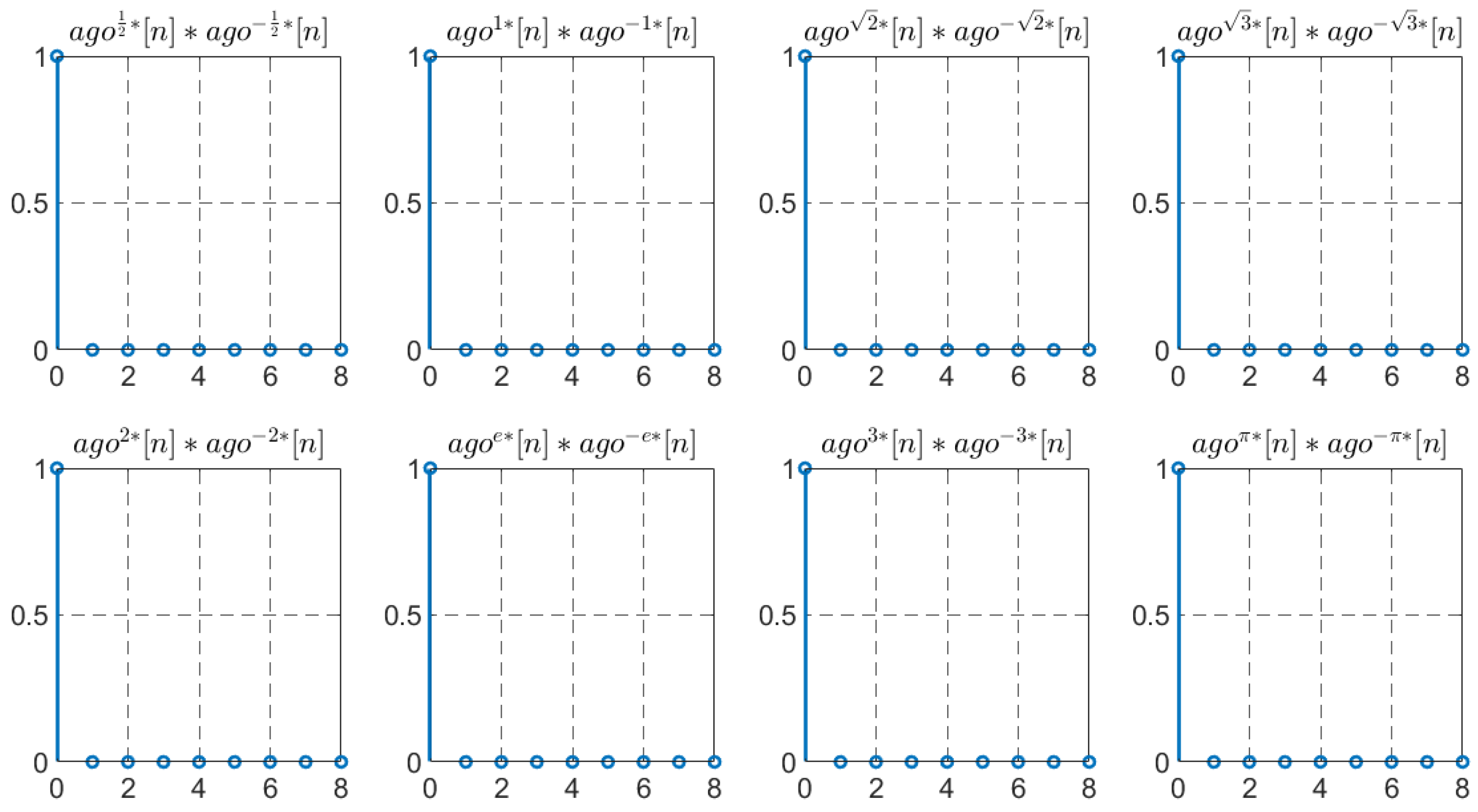
(Mutually inverse relationships). Calculate the convolution of the r-th-order convolution sequences in Case 1 and the inverse -th-order convolution sequences in Case 2 to verify their mutually inverse relationship (21),
with different orders , 1, , , 2, e, 3, π. The convolution operations follow Algorithm 2 and the results are displayed in Figure 3.
Case 4
(Lorenz system [56]). Consider a Lorenz map
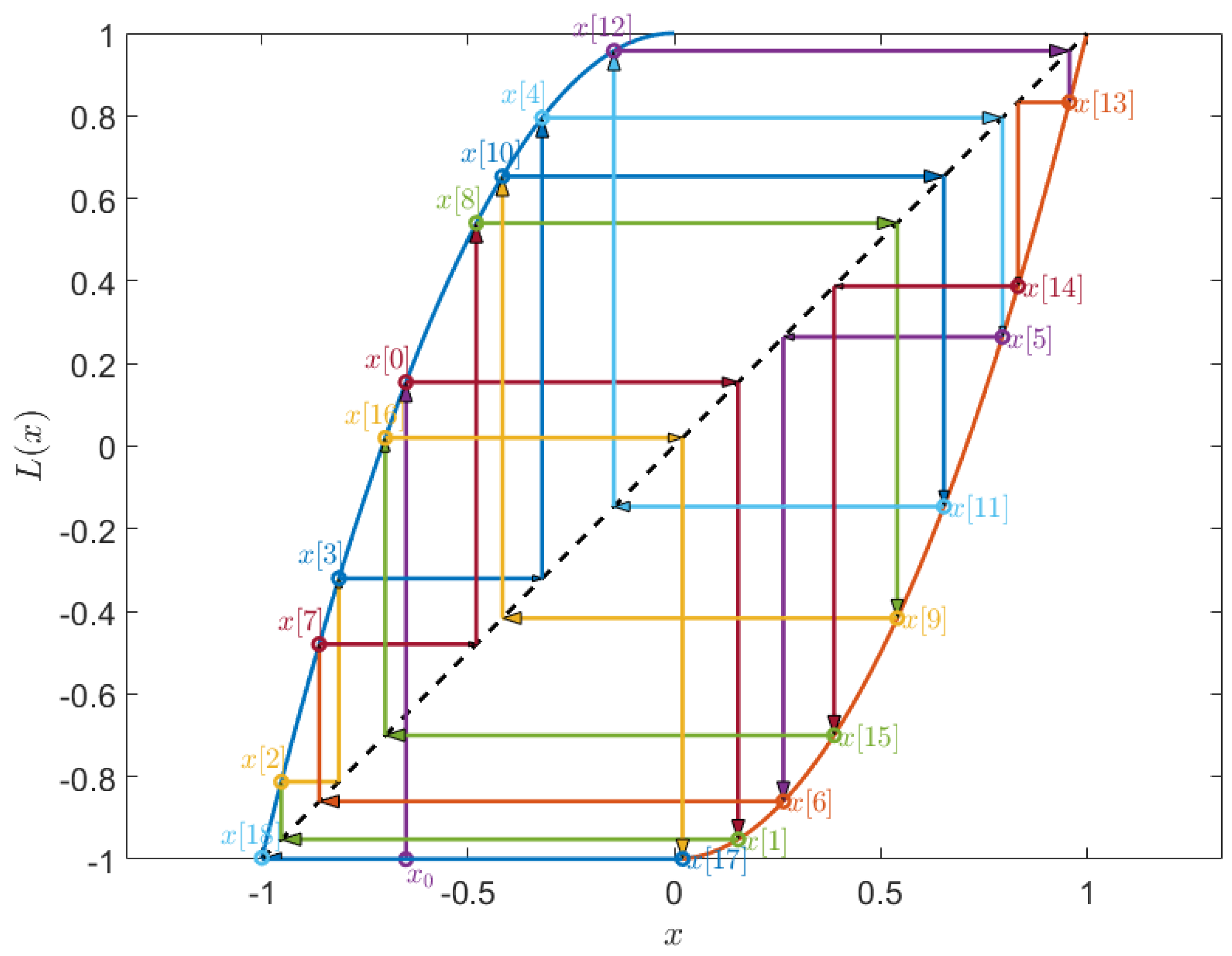
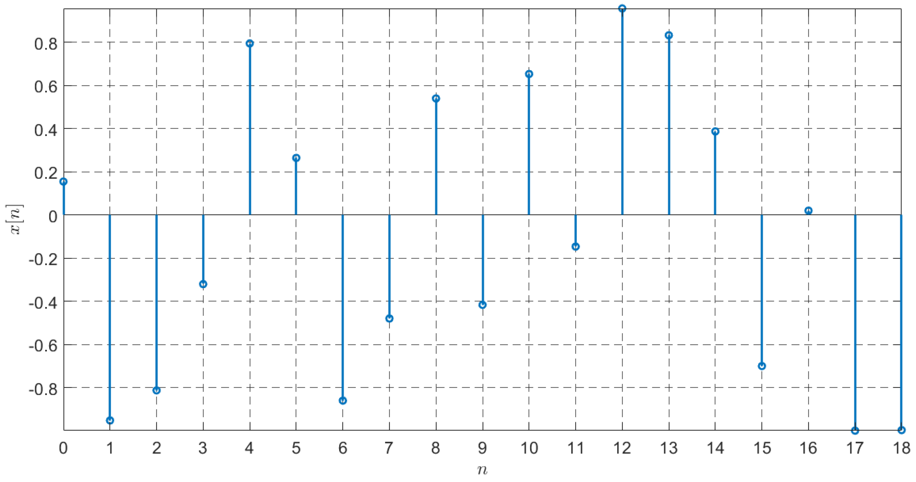
Using (38) as the iterative function, and starting from a random initial point , with 19 iterations, where 16 points checks the model’s coefficient estimation and 3 points check its predictive power. Figure 4 is a cobweb-diagram of the iteration procedure, and the obtained sequence is displayed in Figure 5, illustrating the chaotic characteristic of the sequence obtained from the Lorenz iteration.
The Lorenz system was introduced by a meteorologist, Edward Lorenz, in 1963, describing the unpredictable chaotic motion of convection flow in the atmosphere surrounding the Earth. The Lorenz system, with unstable topological structure, is sensitive to the initial value condition. A small difference at the beginning leads to great unpredictable diversity in the following, which is called “chaos”. Another system family with chaotic features is the one-dimensional map. Guckenheimer and Williams studied the geometric and topological structure of the Lorenz attractor which is a one-dimensional self-map. The chaotic features can also be found in grey models. Tan re-established the context value of the grey model leading to the logistic equation, which mapped the properties of chaos [57].Wang studied the unbiased grey model with chaotic characteristics [58] which improved upon Deng’s model. Zhang applied the grey model to simulate and predict data sequences from a Lorenz chaotic system [56], achieving a predictive precision of over 90%. To make the results comparable with Zhang’s work, the same Lorenz map configuration was used is set as the one in [56].
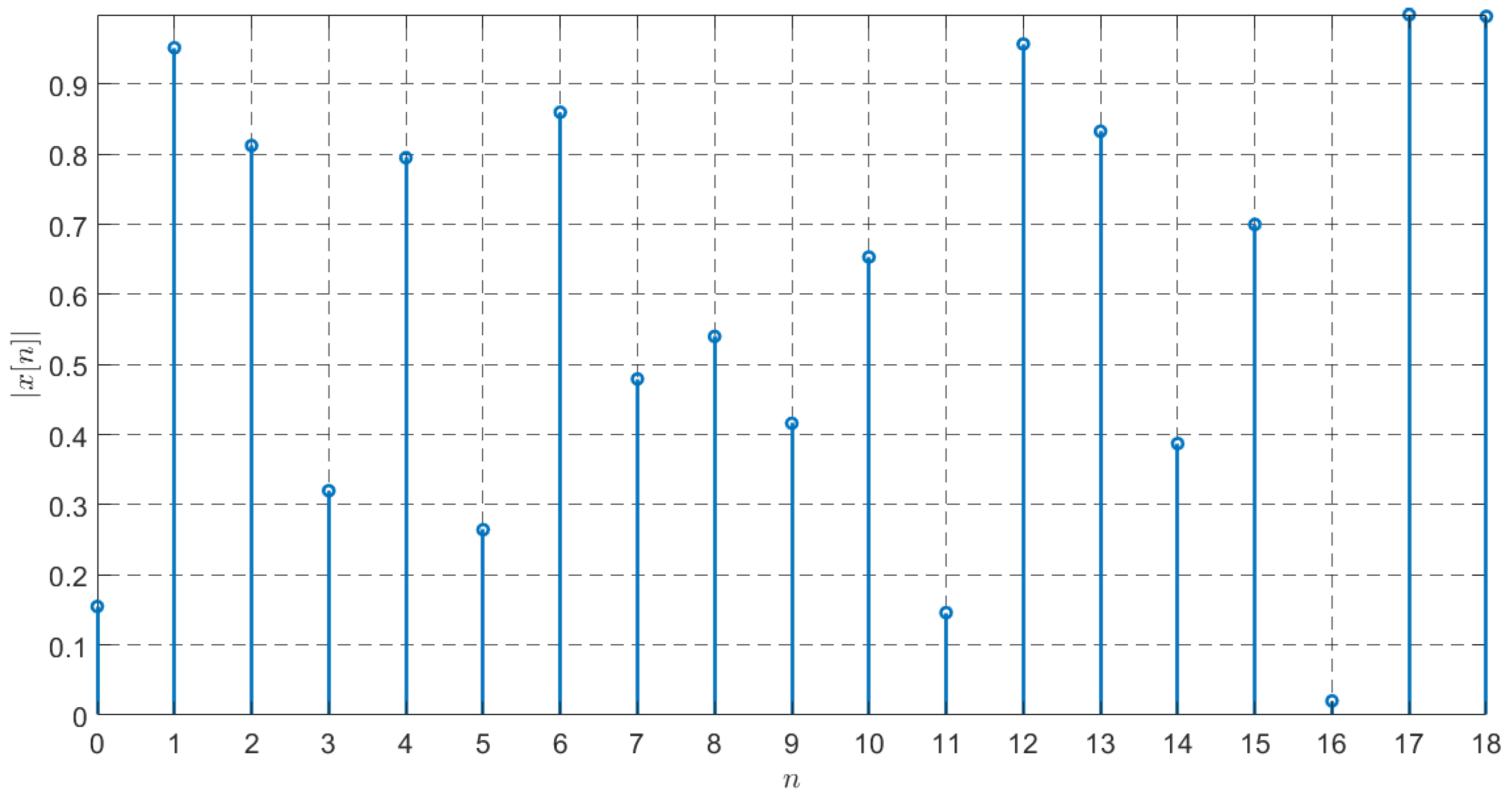
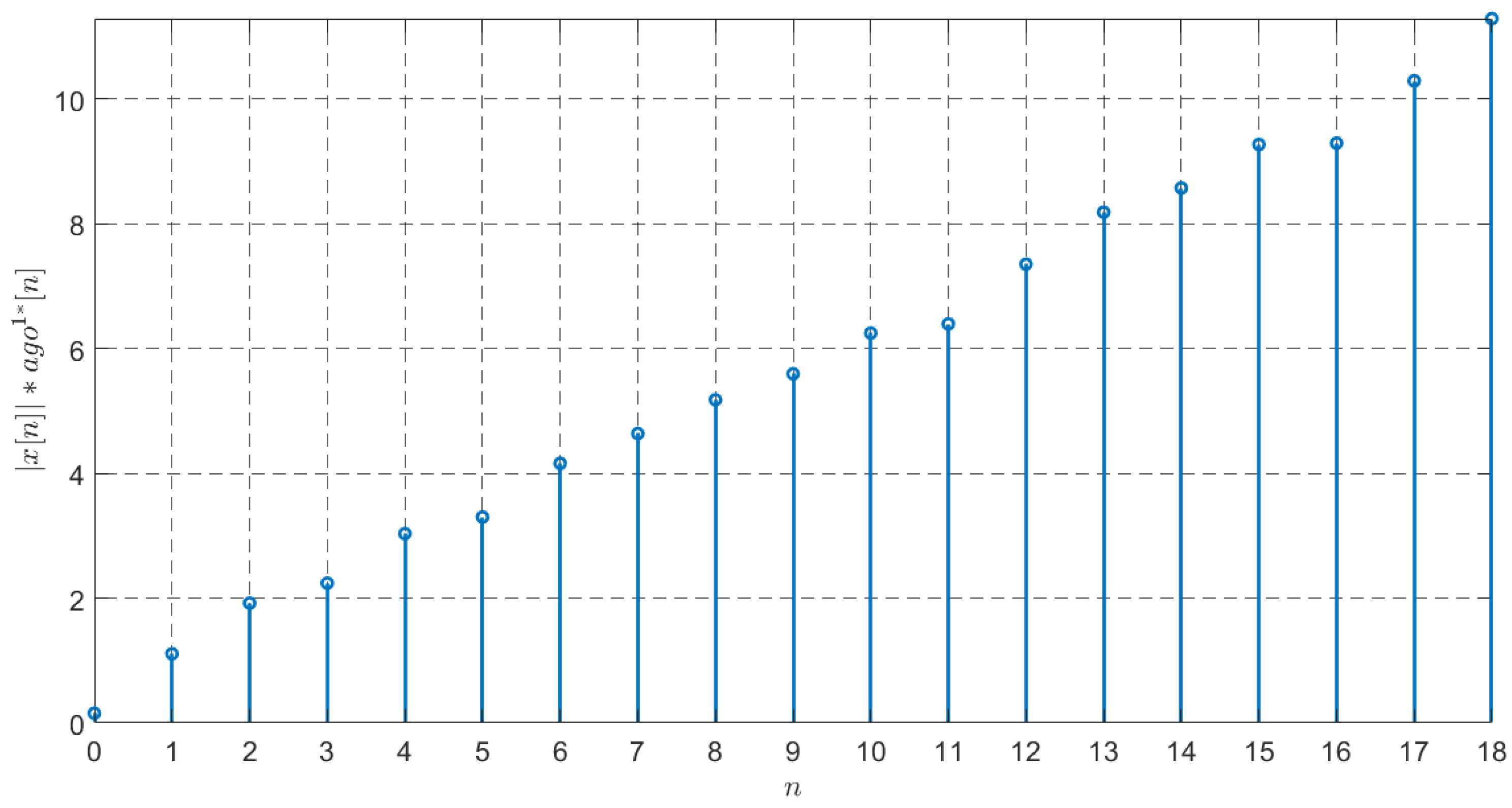
Due to the chaotic characteristics of the Lorenz iteration, two data transforms are employed before grey modeling. Firstly, the absolute values of the Lorenz sequence are taken, denoted by in Figure 6. Secondly, the sequence of absolute values by convolution transform are accumulated, shown in Figure 7. Then the transformed data is denoted as the input sequence to the grey model.
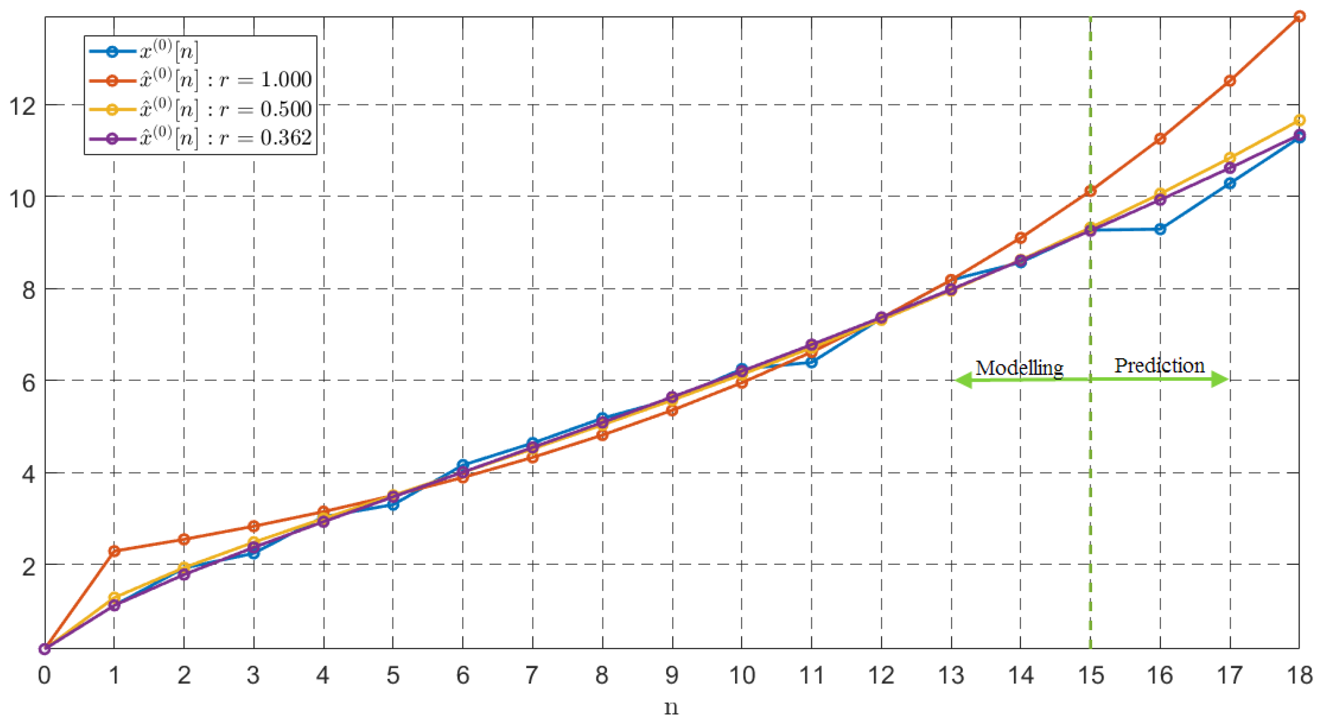
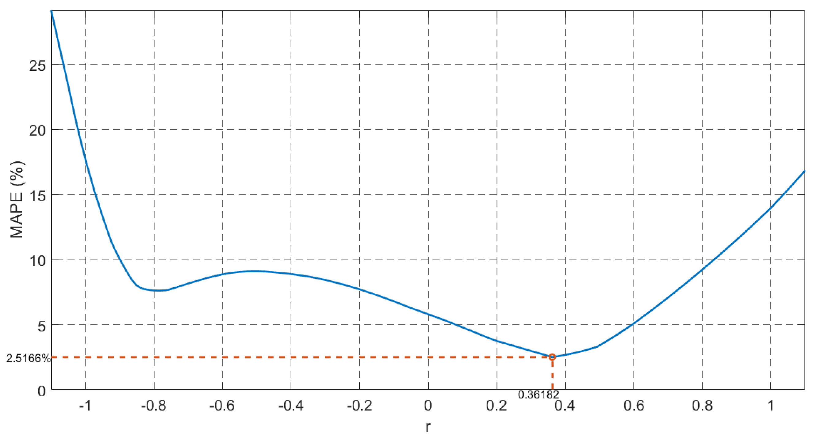
Following Algorithm 1, three different GM models are established with , and . The fitted sequences of the different models are compared with the input sequence in Table 3 and Figure 8. For , it turns out to be the GM model, and its fitted values are the same as those in Zhang’s paper (Table 6 on p. 1008 in [56]). In fact, the in-sample simulation precision was 86% (MAPE in-sample = 13.9748%). This is close to 90% but a little below. However, the out-of-sample predictive precision declinedto 78% (MAPE out-of-sample = 22.0589%). The reason Zhang claimed the precision of the GM model exceeded 90% is that he measured the error at a single datum (Table 6 on p. 1008 in [56]) , which is the local error when he predicted the Lorenz chaotic system; while MAPE belongs to the global error which objectively measures the modelling precision over the whole data sequence. The new fractional-order accumulative convolution grey models are compared with Zhang’s model in Table 3. It can be seen that both grey models with fractional accumulative convolution transform MAPEs are lower than the GM model. Obviously, from Figure 8, two fractional accumulative convolution grey models fitted original data better than ordinary grey model. The MAPE curve with respect to r in Figure 9 demonstrates that is the best fractional-order since the GM achieves the lowest MAPE in-sample, a precision over 97% (MAPE in-sample = 2.5166%), and gives the best prediction out-of-sample, over 96% (MAPE out-of-sample = 3.5414%).
Case 5.
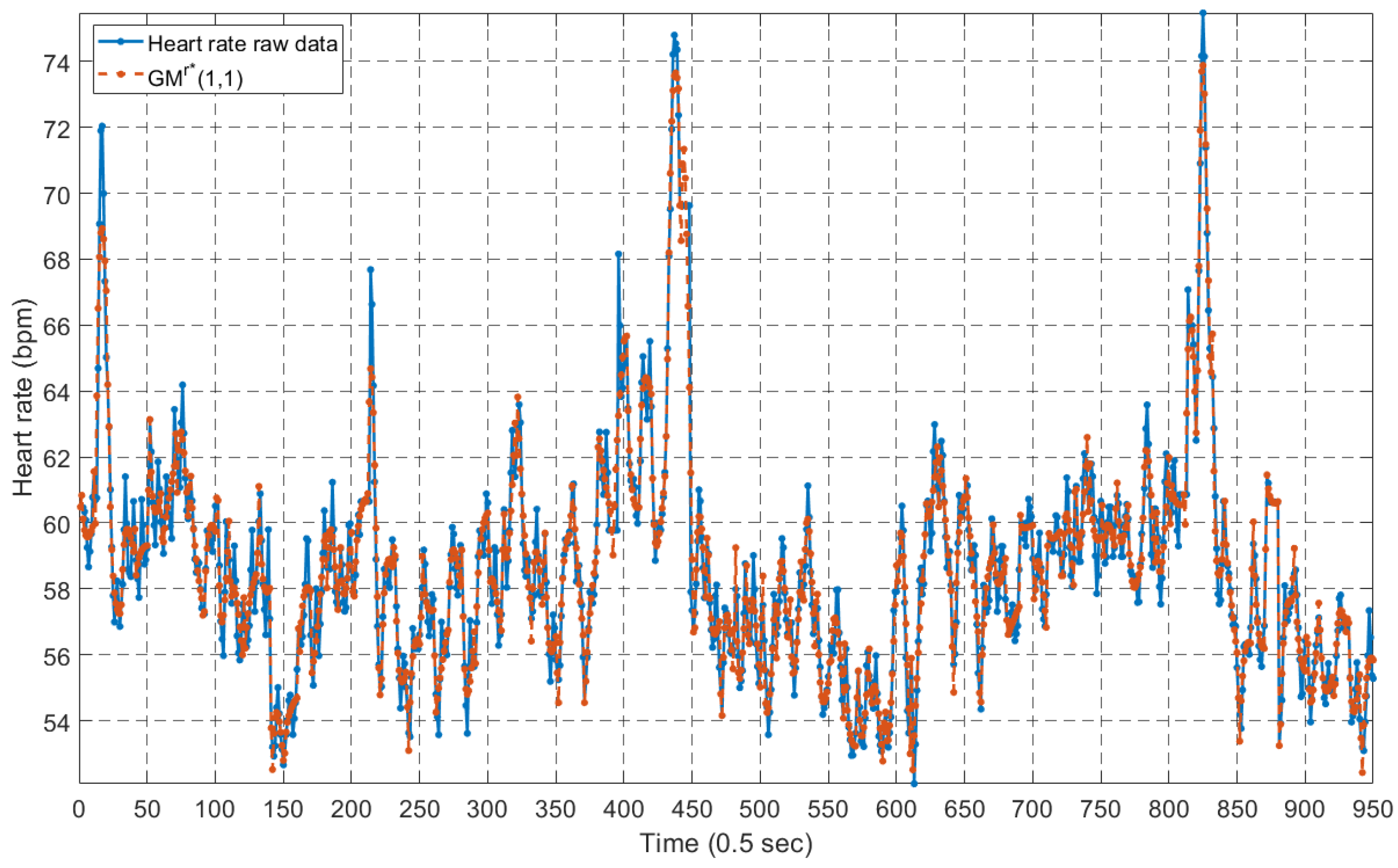
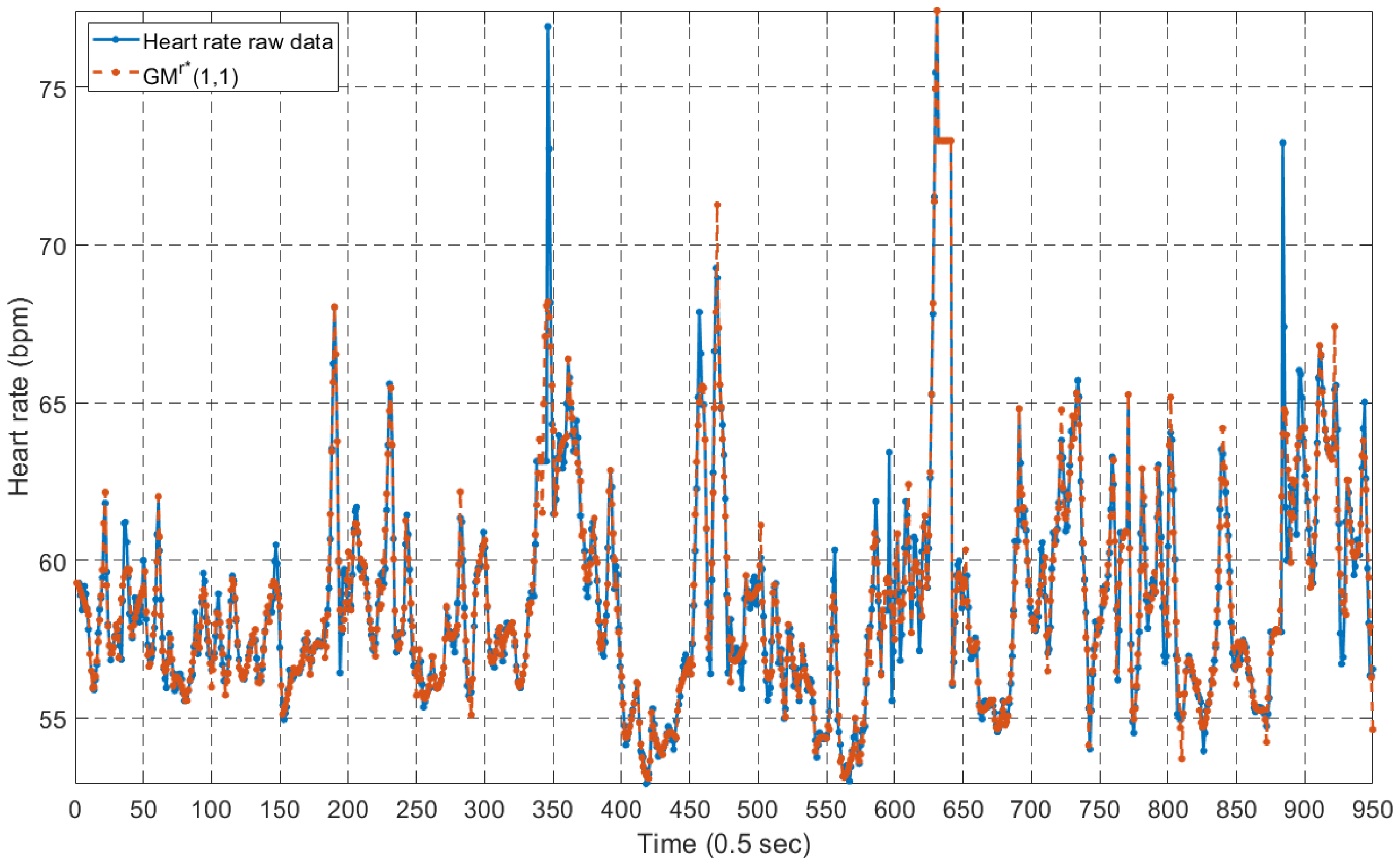
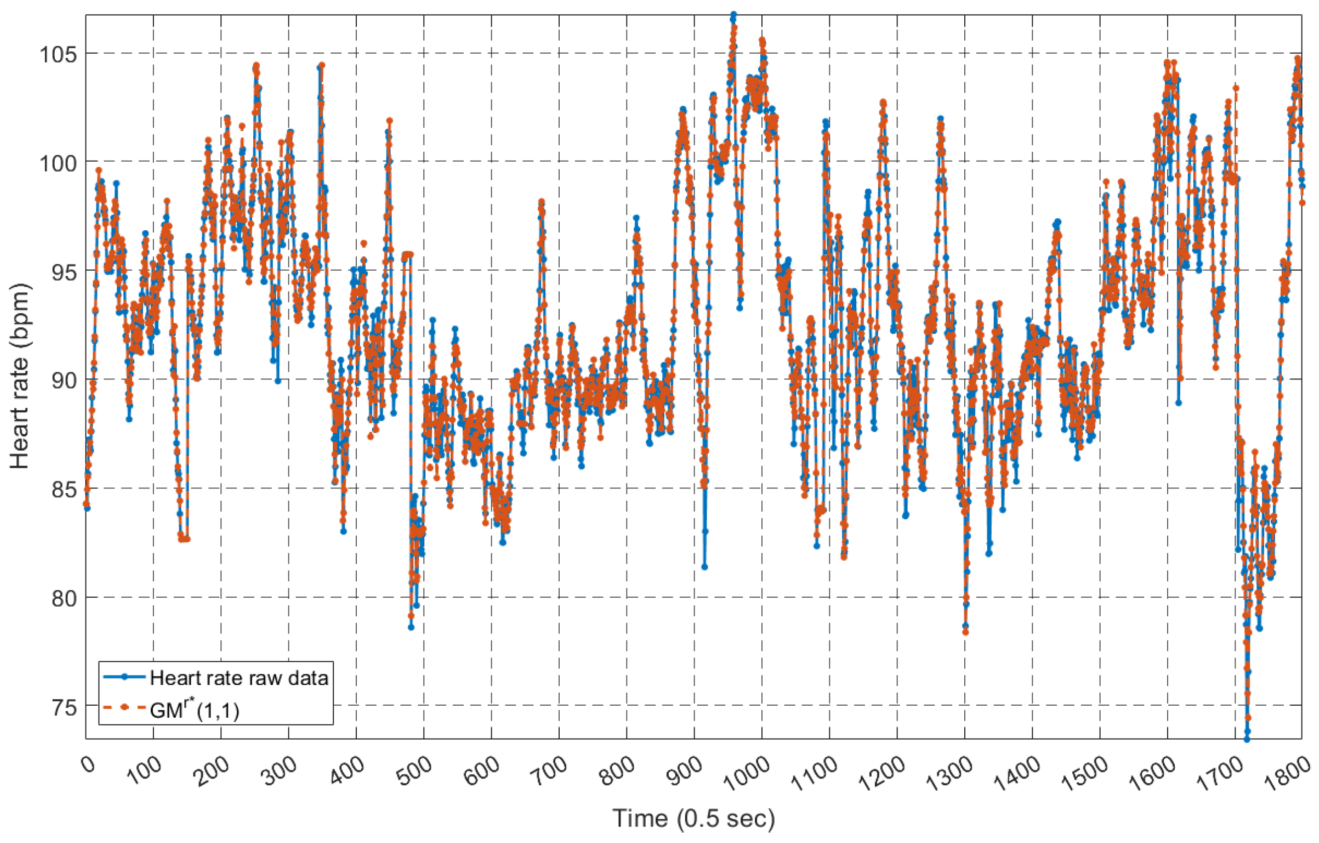
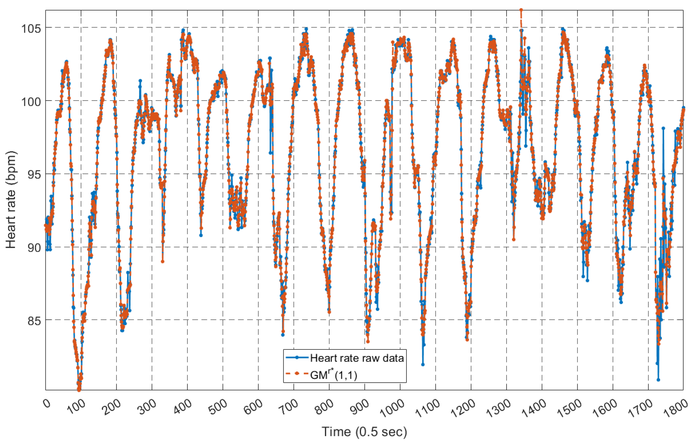
Consider time sequences of the electrocardiogram (ECG), which can be downloaded from the MIT-BIH Database [59]. Four ECG sequences: “hr.207”, “hr.237”, “hr.11839” and “hr.7257” are studied here. Sequences “hr.207” and “hr.237” contain 950 measured points of the transient heart rate (unit: beats per minute); while sequences “hr.11839” and “hr.7257” contain 1800 points. The time spacing between the measure points is 0.5 s.
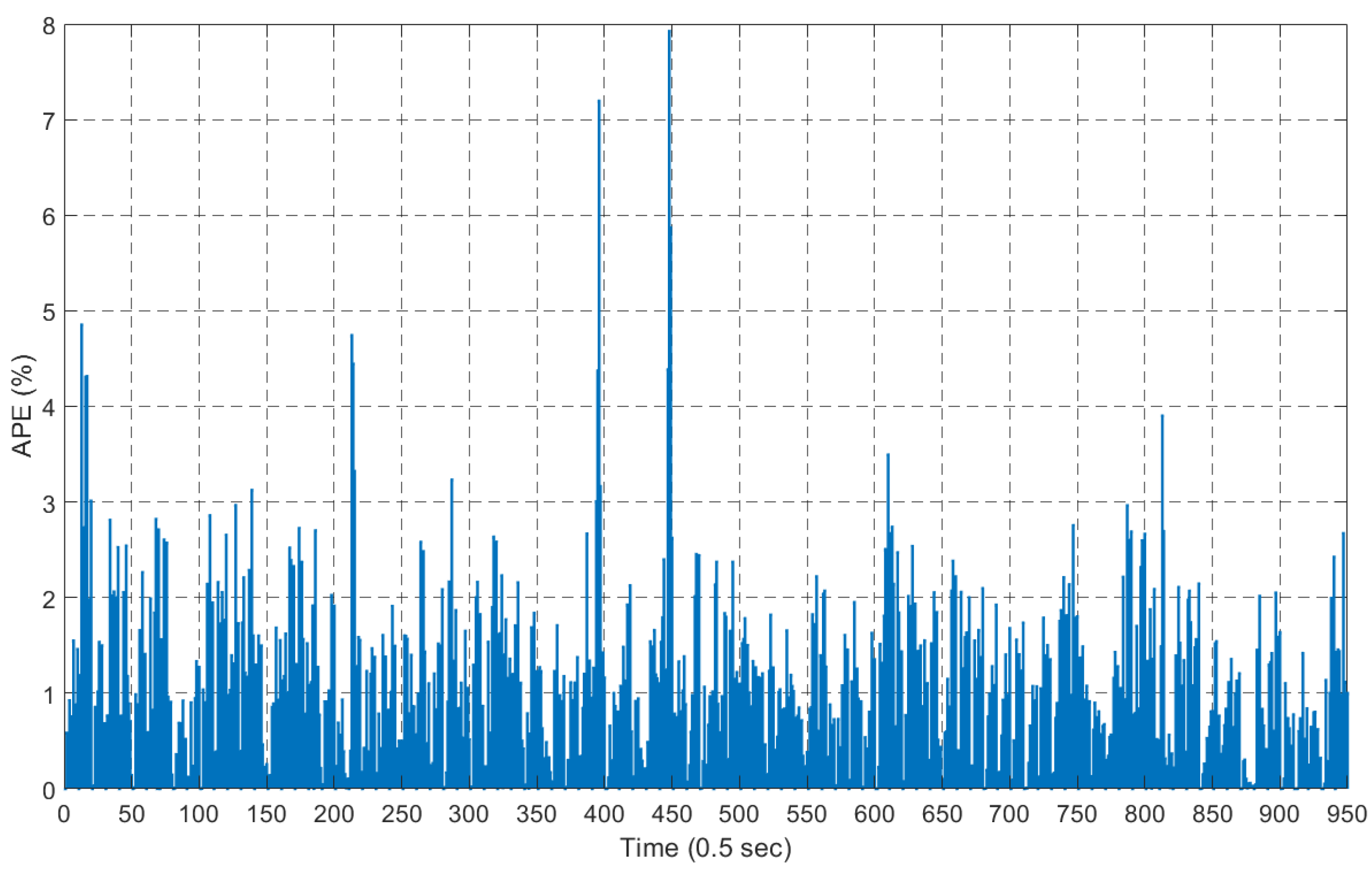
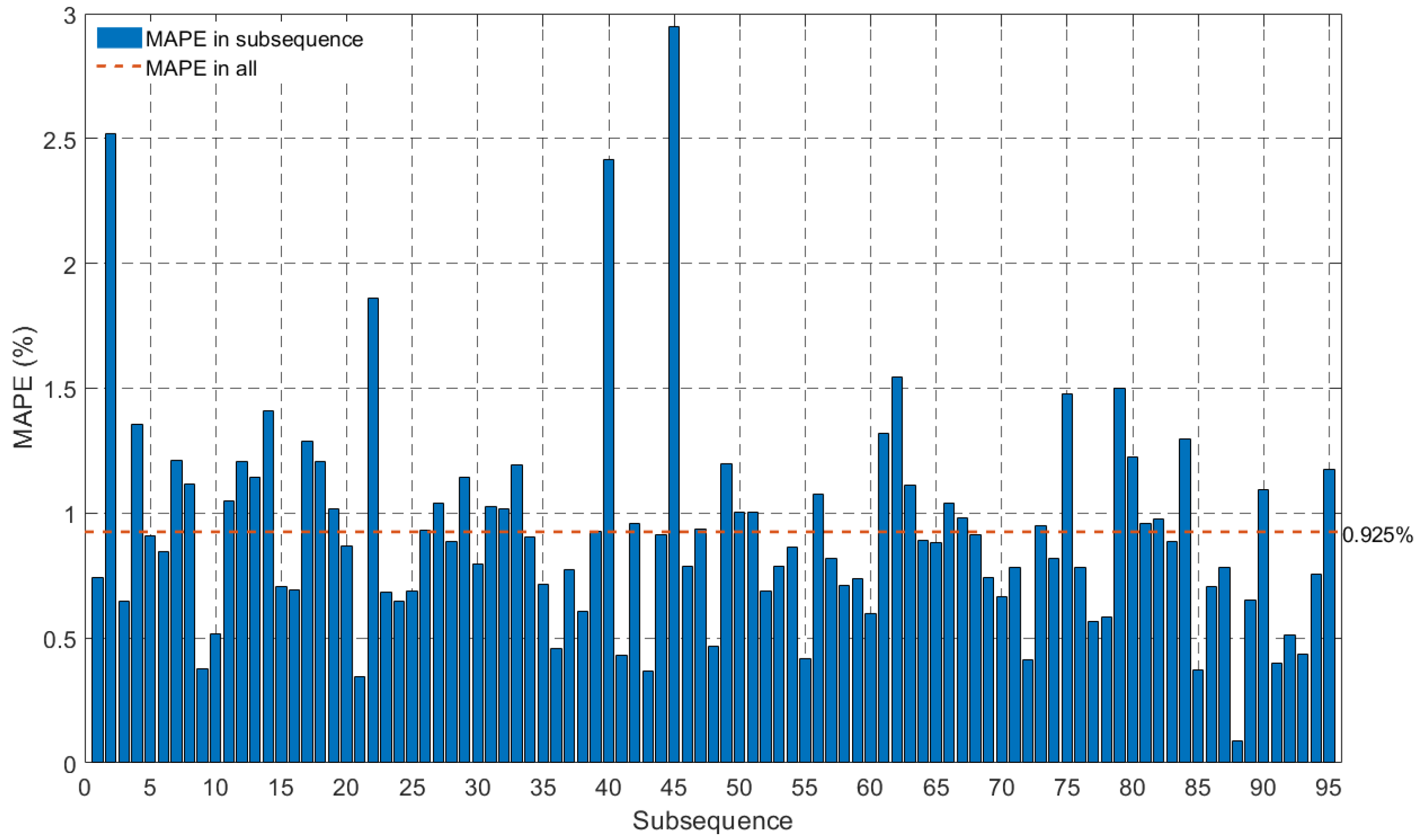
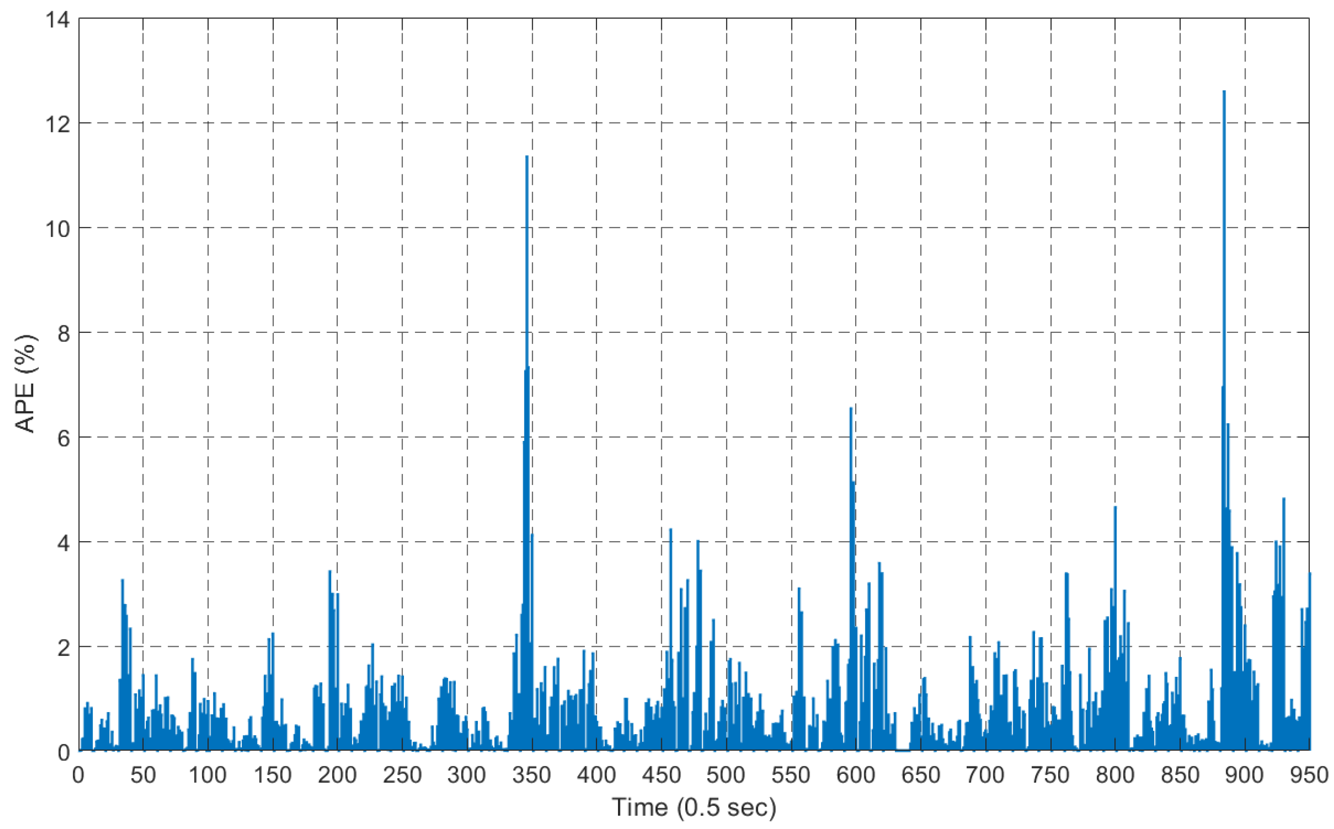
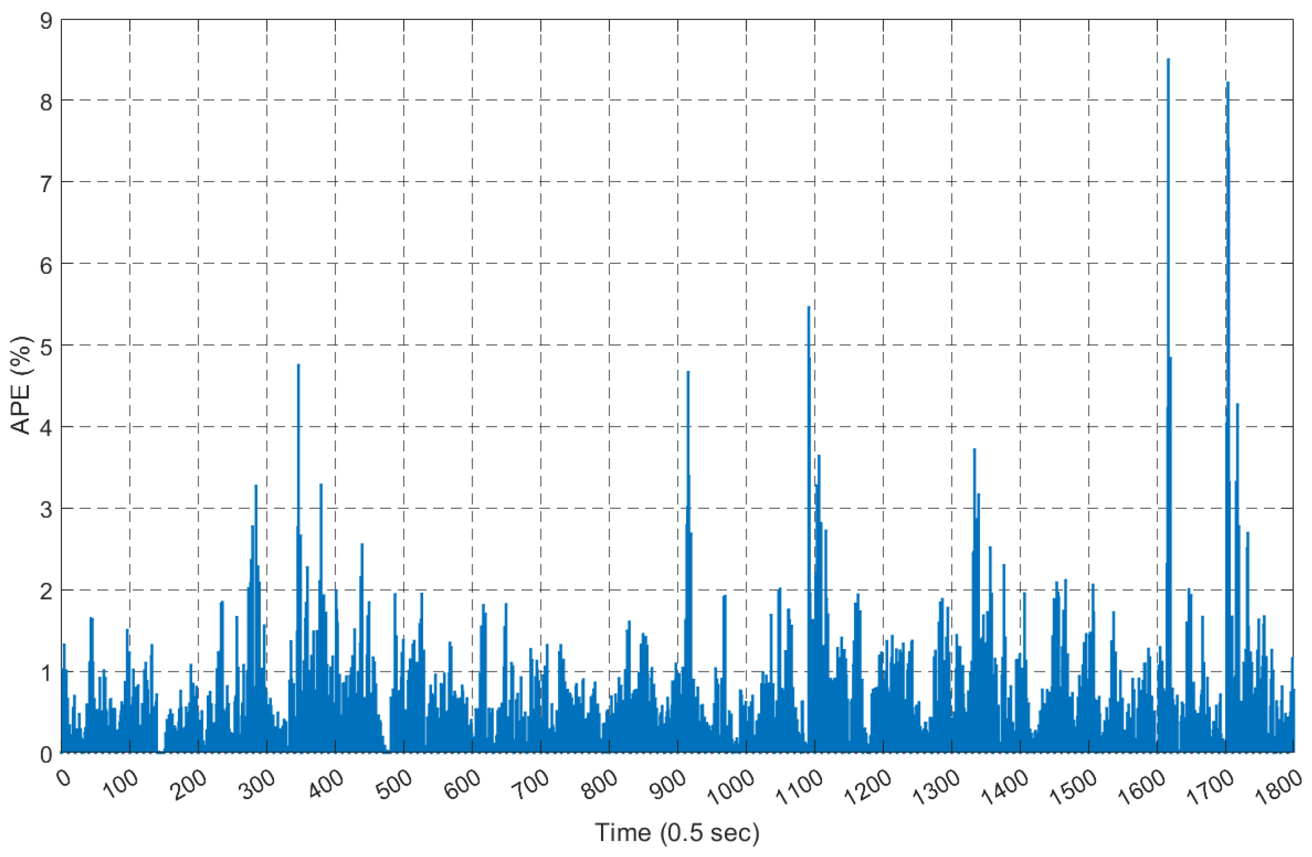
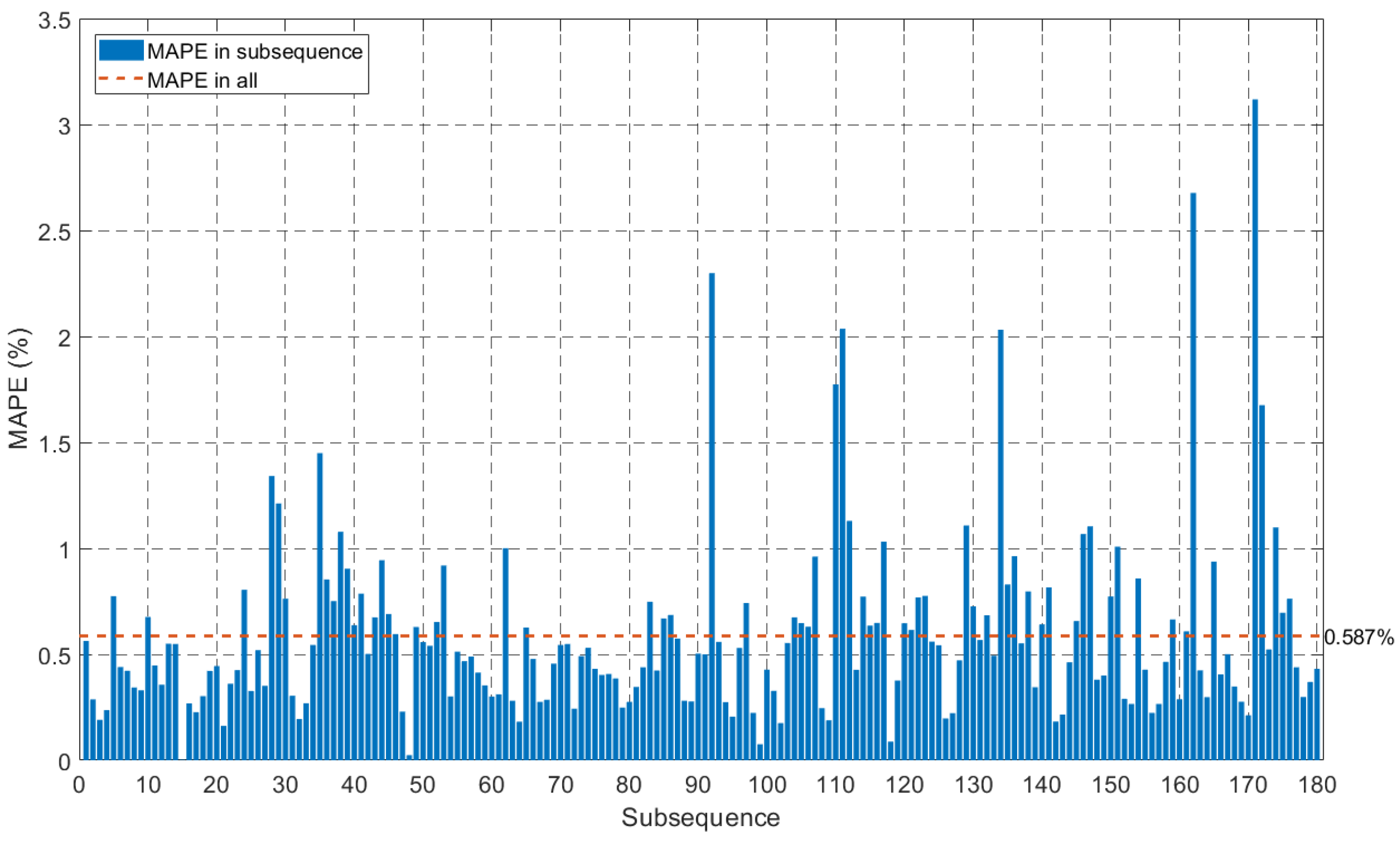
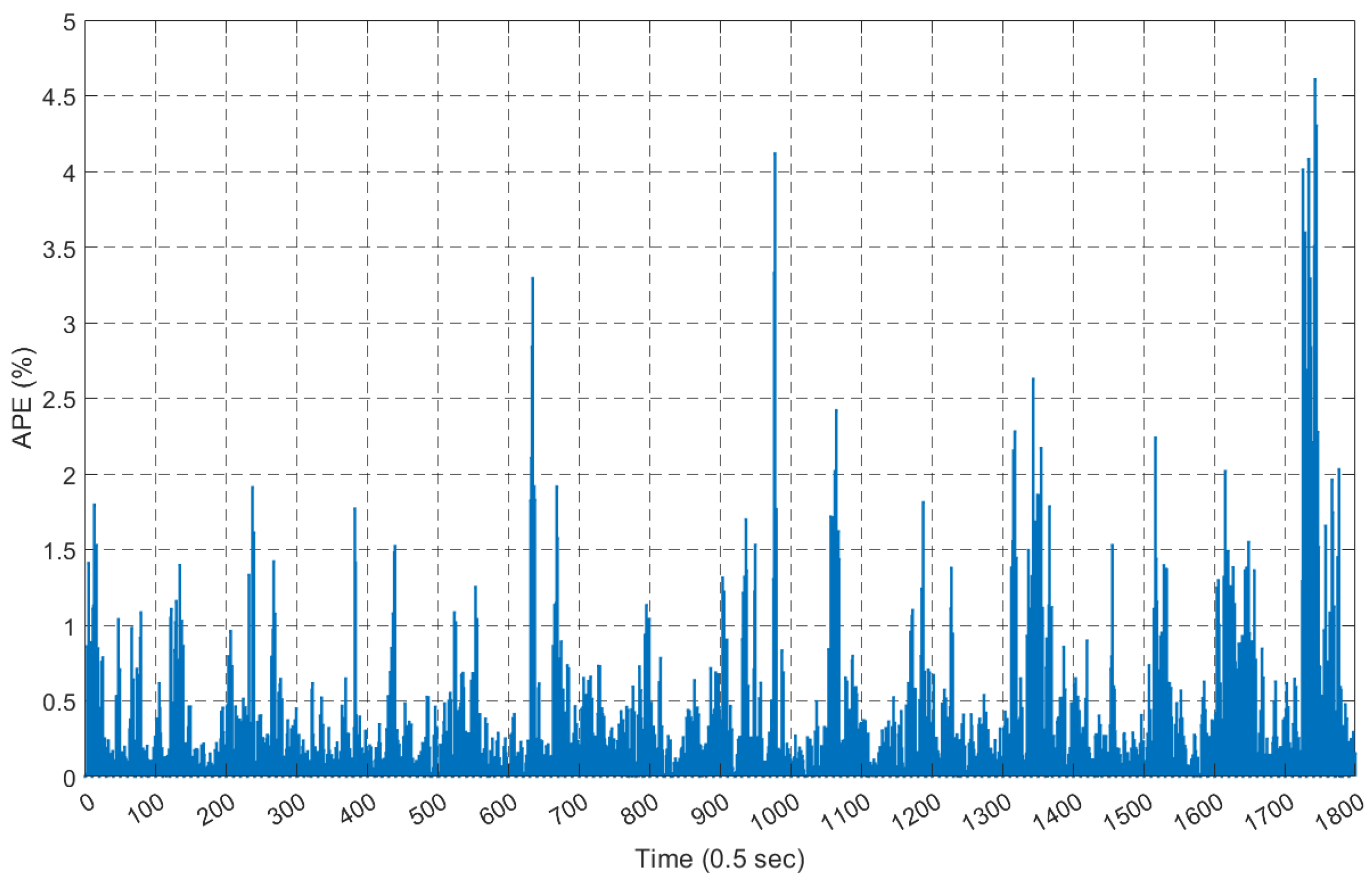
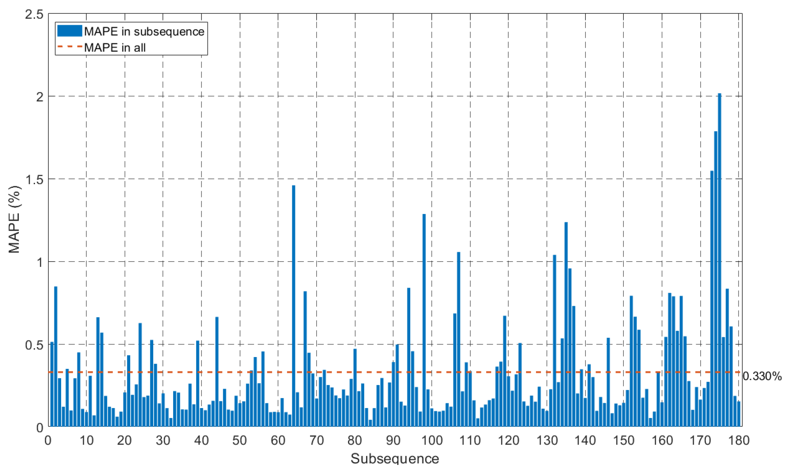
Figure 10 shows the fitted results from the GM model compared with the original ECG sequence “hr.207”. Figure 11 represents the absolute percentage error (APE) of the fitting at each sampling point. Furthermore, Figure 12 is the mean absolute percentage error (MAPE) of the fitting in each sample block, containing 10 sampling points. Similarly, Figure 13, Figure 14 and Figure 15 display the ECG sequence for “hr.237”. Figure 16, Figure 17 and Figure 18 display the ECG sequence for “hr.11839”. Figure 19, Figure 20 and Figure 21 display the ECG sequence for “hr.7257”.
5. Conclusions
The accumulation generation and its inversion are essential procedures in grey modelling. They are implemented here in a new way—sequence convolution. The fractional-order accumulative convolution sequence is constructed to fulfil the fractional-order accumulative generation procedure. Based on accumulative convolution, the fractional accumulative convolution grey model is established. The main results of this paper are as follows.
- (i)
- The accumulative generation convolution sequence is constructed by the unit impulse sequence in Theorem 1. The classical accumulative generation procedure can be fulfilled by the sequence convolution, i.e., yields to accumulated sequence, and its inverse, returns to the original sequence. They are mutually inverse in the sense of convolution operation, i.e., .
- (ii)
- The fractional-order accumulative convolution sequence is constructed in Theorem 3. With the convolution transform, yields to the fractional accumulated sequence , and with the convolution transform of its inverse sequence, recovers the data. Furthermore, the two fractional-order accumulative convolution sequences are mutually inverse in the convolution operation, .
- (iii)
- Under the fractional-order accumulative convolution transform, the new GM is established in Algorithm 1. The cases above verify and demonstrate the validity and effectiveness of the new model.
Accumulative convolution transform and its inversion are new concepts for data transformation. The success in the grey forecasting GM model is one application of the fractional-order accumulative convolution transformation. It could be found in more extensive applications in other disciplines. Some possible research directions in the future are listed as follows.
- (i)
- Since the unit impulse response of the fractional-order accumulative system has been obtained, the powerful tools in digital signal process could be used to analysis the more impressive properties of the fractional-order accumulative system.
- (ii)
- Fractional-order accumulative convolution transform is the discrete form of integration, and can be applied in fractional calculus and fractional differential equations.
Funding
The Fundamental Research Funds for the Central Universities.
Institutional Review Board Statement
The study did not require ethical approval.
Data Availability Statement
Publicly available datasets were analysed in this study. This data can be found at: http://ecg.mit.edu/time-series/index.html (accessed on 5 May 2023).
Conflicts of Interest
The authors declare no conflict of interest.
References
- Deng, J. Introduction Grey System Theory. J. Grey Syst. 1989, 1, 1–24. [Google Scholar]
- Putter, H.; Heisterkamp, S.H.; Lange, J.M.A.; de Wolf, F. A Bayesian Approach to Parameter Estimation in HIV Dynamical Models. Stat. Med. 2022, 21, 2199–2214. [Google Scholar] [CrossRef]
- Zhang, G.; Sheng, Y. Maximum Likelihood Estimation of Time-Varying Parameters in Uncertain Differential Equations. J. Xinjiang Univ. (Nat. Sci. Ed. Chin. Engl.) 2022, 39, 421–431. (In Chinese) [Google Scholar]
- Jamili, E.; Dua, V. Parameter estimation of partial differential equations using artificial neural network. Comput. Chem. Eng. 2021, 147, 107221. [Google Scholar] [CrossRef]
- Torres, M. A Machine Learning Method for Parameter Estimation and Sensitivity Analysis. In Proceedings of the Computational Science-ICCS 2021, Krakow, Poland, 16–18 June 2021; Lecture Notes in Computer Science; Paszynski, M., Kranzlmuller, D., Krzhizhanovskaya, V., Dongarra, J., Sloot, P., Eds.; Springer: Cham, Switzerland, 2021; Volume 12746, pp. 330–343. [Google Scholar]
- Deng, J. Grey Control System, 2nd ed.; Press of Huazhong University of Science and Technology: Wuhan, China, 1993. (In Chinese) [Google Scholar]
- Yao, T.; Liu, S.; Xie, N. On the properties of small sample of GM(1,1) model. Appl. Math. Model. 2009, 33, 1894–1903. [Google Scholar] [CrossRef]
- Wu, L.; Liu, S.; Yao, L.; Yan, S. The effect of sample size on the grey system model. Appl. Math. Model. 2013, 37, 6577–6583. [Google Scholar] [CrossRef]
- Zhicun, X.; Meng, D.; Lifeng, W. Evaluating the effect of sample length on forecasting validity of FGM(1,1). Alex. Eng. J. 2020, 59, 4687–4698. [Google Scholar] [CrossRef]
- Wang, Z. Grey forecasting method for small sample oscillating sequences based on Fourier series. Control Decis. 2014, 29, 270–274. (In Chinese) [Google Scholar]
- Talafuse, T.P.; Pohl, E.A. Small sample discrete reliability growth modeling using a grey systems model. Grey Syst. Theory Appl. 2018, 8, 246–271. [Google Scholar] [CrossRef]
- Ma, X.; Liu, Z.b. The kernel-based nonlinear multivariate grey model. Appl. Math. Model. 2018, 56, 217–238. [Google Scholar] [CrossRef]
- Liu, S.; Tao, Y.; Xie, N.; Tao, L.; Hu, M. Advance in grey system theory and applications in science and engineering. Grey Syst. Theory Appl. 2022, 12, 804–823. [Google Scholar] [CrossRef]
- Hu, M.; Liu, W. Grey system theory in sustainable development research—A literature review (2011–2021). Grey Syst. Theory Appl. 2022, 12, 785–803. [Google Scholar] [CrossRef]
- Xiao, X.; Duan, H. A new grey model for traffic flow mechanics. Eng. Appl. Artif. Intell. 2020, 88, 103350. [Google Scholar] [CrossRef]
- Seneviratna, D.; Rathnayaka, R.K.T. Hybrid grey exponential smoothing approach for predicting transmission dynamics of the COVID-19 outbreak in Sri Lanka. Grey Syst. Theory Appl. 2022, 12, 824–838. [Google Scholar] [CrossRef]
- Camelia, D. Grey systems theory in economics—A historical applications review. Grey Syst. Theory Appl. 2015, 5, 263–276. [Google Scholar] [CrossRef]
- Li, X.; Cao, Y.; Wang, J.; Dang, Y.; Kedong, Y. A summary of grey forecasting and relational models and its applications in marine economics and management. Grey Syst. Theory Appl. 2019, 2, 87–113. [Google Scholar]
- Huang, J.; Wang, R.; Shi, Y. Urban climate change: A comprehensive ecological analysis of the thermo-effects of major Chinese cities. Ecol. Complex. 2010, 7, 188–197. [Google Scholar] [CrossRef]
- Li, B.; Zhang, S.; Li, W.; Zhang, Y. Application progress of grey model technology in agricultural science. Grey Syst. Theory Appl. 2022, 12, 744–784. [Google Scholar] [CrossRef]
- Liu, S.; Yang, Y.; Wu, L. Grey System Theory and Application; Science Press: Beijing, China, 2014. [Google Scholar]
- Liu, S.; Yang, Y.; Forrest, J. Grey Data Analysis: Methods, Models and Applications; Springer: Singapore, 2017. [Google Scholar]
- Xie, N.; Wang, R. A historic review of grey forecasting models. J. Grey Syst. 2017, 29, 1–29. [Google Scholar]
- Xie, N. A summary of grey forecasting models. Grey Syst. Theory Appl. 2022, 12, 703–722. [Google Scholar] [CrossRef]
- Deng, J. Grey Forecasting and Decision-Making; Press of Huazhong University of Science and Technology: Wuhan, China, 1986. (In Chinese) [Google Scholar]
- Liu, S.; Lin, Y. Grey Systems: Theory and Applications; Springer: Berlin/Heidelberg, Germany, 2010. [Google Scholar]
- Liu, S. The three axioms of buffer operator and their application. J. Grey Syst. 1991, 3, 39–48. [Google Scholar]
- Makhlouf, A.B.; Naifar, O.; Hammami, M.A.; Wu, B. FTS and FTB of Conformable Fractional Order Linear Systems. Math. Probl. Eng. 2018, 2018, 2572986. [Google Scholar] [CrossRef]
- Naifar, O.; Boukettaya, G.; Oualha, A.; Ouali, A. A comparative study between a high-gain interconnected observer and an adaptive observer applied to IM-based WECS. Eur. Phys. J. Plus 2015, 130, 88. [Google Scholar] [CrossRef]
- Ayadi, M.; Naifar, O.; Derbel, N. High-order sliding mode control for variable speed PMSG-wind turbine-based disturbance observer. Int. J. Model. Identif. Control 2019, 32, 85–92. [Google Scholar] [CrossRef]
- Wu, L.; Liu, S.; Yao, L. Grey model with Caputo fractional order derivative. Syst. Eng.—Theory Prat. 2015, 35, 1311–1316. (In Chinese) [Google Scholar]
- Ma, X.; Wu, W.; Zeng, B.; Wang, Y.; Wu, X. The conformable fractional grey system model. ISA Trans. 2020, 96, 255–271. [Google Scholar] [CrossRef]
- Wu, L.; Liu, S.; Chen, D.; Yao, L. Using gray model with fractional order accumulation to predict gas emission. Nat. Hazards 2014, 71, 2231–2236. [Google Scholar] [CrossRef]
- Wu, W.; Ma, X.; Zhang, Y.; Li, W.; Wang, Y. A novel conformable fractional non-homogeneous grey model for forecasting carbon dioxide emissions of BRICS countries. Sci. Total. Environ. 2020, 707, 135447. [Google Scholar] [CrossRef]
- Wu, L.; Liu, S.; Yao, L.; Yan, S.; Liu, D. Grey system model with the fractional order accumulation. Commun. Nonlinear Sci. Numer. Simul. 2013, 252, 1775–1785. [Google Scholar] [CrossRef]
- Wu, L.; Liu, S.; Yao, L.; Xu, R.; Lei, X. Using fractional order accumulation to reduce errors from inverse accumulated generating operator of grey model. Soft Comput. 2014, 252, 1775–1785. [Google Scholar] [CrossRef]
- Wu, L.; Liu, S.; Fang, Z.; Xu, H. Properties of the GM(1,1) with fractional order accumulation. Appl. Math. Comput. 2015, 252, 287–293. [Google Scholar] [CrossRef]
- Wu, L. Using fractional GM(1,1) model to predict the life of complex equipment. Grey Syst. Theory Appl. 2016, 6, 32–40. [Google Scholar] [CrossRef]
- Xiao, X.; Guo, H.; Mao, S. The modeling mechanism, extension and optimization of grey GM(1,1) model. Appl. Math. Model. 2014, 38, 1896–1910. [Google Scholar] [CrossRef]
- Mao, S.; Gao, M.; Xiao, X. A Novel Fractional Grey System Model and its Application. Appl. Math. Model. 2016, 40, 5063–5076. [Google Scholar] [CrossRef]
- Meng, W.; Zeng, B. Discrete Grey Model with Inverse Fractional Operators and Optimized Order. Control Decis. 2016, 31, 1903–1907. (In Chinese) [Google Scholar]
- Meng, W.; Zeng, B.; Li, S. A Novel Fractional-Order Grey Prediction Model and Its Modeling Error Analysis. Information 2016, 10, 167. [Google Scholar] [CrossRef]
- Zeng, B.; YU, L.; Liu, S.; Meng, W.; Zhou, M. Unification of grey accumulation operator and the inverse operator and its application. Information 2021, 41, 2710–2720. [Google Scholar]
- Wu, Z.; Chen, J.; Chai, J.; Zhang, F. Grey System Model with Complex Order Accumulation. J. Grey Syst. 2021, 33, 98–117. [Google Scholar]
- Wei, B.; Xie, N.; Yang, L. Understanding cumulative sum operator in grey prediction model with integral matching. Commun. Nonlinear Sci. Numer. Simul. 2020, 82, 105076. [Google Scholar] [CrossRef]
- Wei, B.; Xie, N. On unified framework for discrete-time grey models: Extension and applications. ISA Trans. 2020, 107, 1–11. [Google Scholar] [CrossRef]
- Wei, B.; Xie, N. On unified framework for continuous-time grey models: An integral matching perspective. Appl. Math. Model. 2022, 101, 432–452. [Google Scholar] [CrossRef]
- Chen, C. Improvement on the AGO and a Grey Model GM(1,1,t). Math. Pract. Theory 2007, 37, 105–109. (In Chinese) [Google Scholar]
- Lin, C.; Wang, Y.; Liu, S.; Zhang, Y.; Tao, L. On Spectrum Analysis of Different Weakening Buffer Operators. J. Grey Syst. 2019, 31, 111–121. [Google Scholar]
- Liu, S.; Lin, C.; Tao, L.; Javed, S.A.; Fang, Z.; Yang, Y. On Spectral Analysis and New Research Directions in Grey System Theory. J. Grey Syst. 2020, 32, 108–117. [Google Scholar]
- Lin, C.; Song, Z.; Liu, S.; Yang, Y.; Forrest, J. Study on mechanism and filter efficacy of AGO/IAGO in the frequency domain. Grey Syst. Theory Appl. 2021, 11, 1–21. [Google Scholar] [CrossRef]
- Lin, C.; Liu, S.; Fang, Z.; Yang, Y. Spectrum analysis of moving average operator and construction of time-frequency hybrid sequence operator. Grey Syst. Theory Appl. 2022, 12, 101–116. [Google Scholar] [CrossRef]
- Proakis, J.G.; Manolakis, D.G. Digital Signal Process: Principles, Algorithms and Applications, 4th ed.; Pearson Prentice Hall: Upper Saddle River, NJ, USA, 2006. [Google Scholar]
- Hirschman, I.I.; Widder, D.V. The Convolution Transform; Princeton University Press: Princeton, NJ, USA, 1955. [Google Scholar]
- Leng, J. Fourier Transformation; Tsinghua University Press: Beijing, China, 2004. (In Chinese) [Google Scholar]
- Zhang, Y.; Yan, X.; Wang, Z. GM(1,1) Grey prediction of Lorenz chaotic system. Chaos Solitons Fractals 2009, 42, 1003–1009. [Google Scholar] [CrossRef]
- Tan, G. The Structure Method Application of Background Value in Grey System GM(1,1) Model (III). Syst. Eng.—Theory Pract. 2000, 6, 70–74. (In Chinese) [Google Scholar]
- Wang, Z.; Dang, Y.; Liu, S. Analysis of Chaotic Charateristics of Unbiased GM(1,1). Syst. Eng.—Theory Pract. 2007, 11, 153–158. (In Chinese) [Google Scholar]
- Heart Rate Time Series. Available online: http://ecg.mit.edu/time-series/index.html (accessed on 5 May 2023).
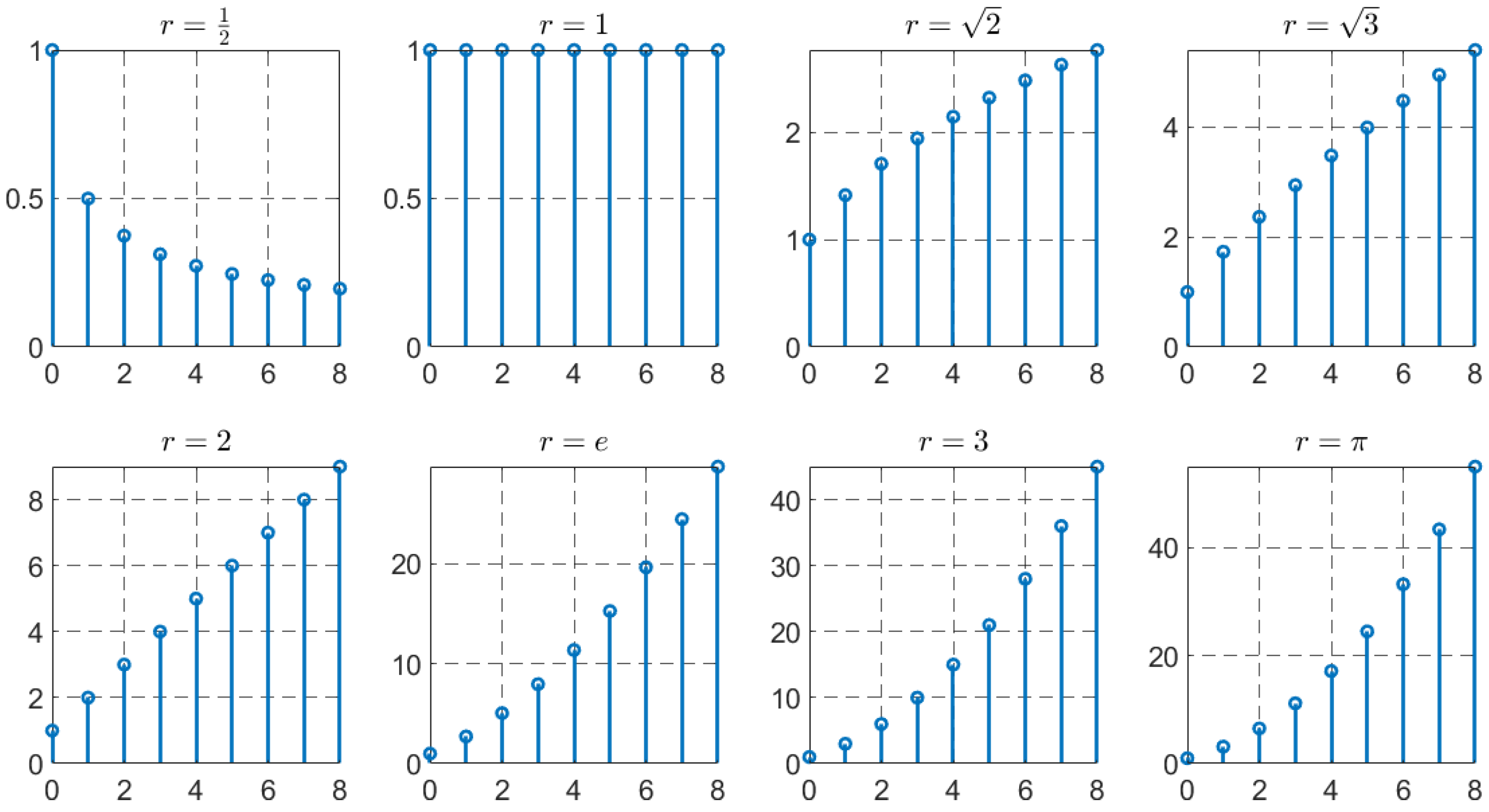
Figure 1.
Accumulative convolution sequences with fractional r-th order.

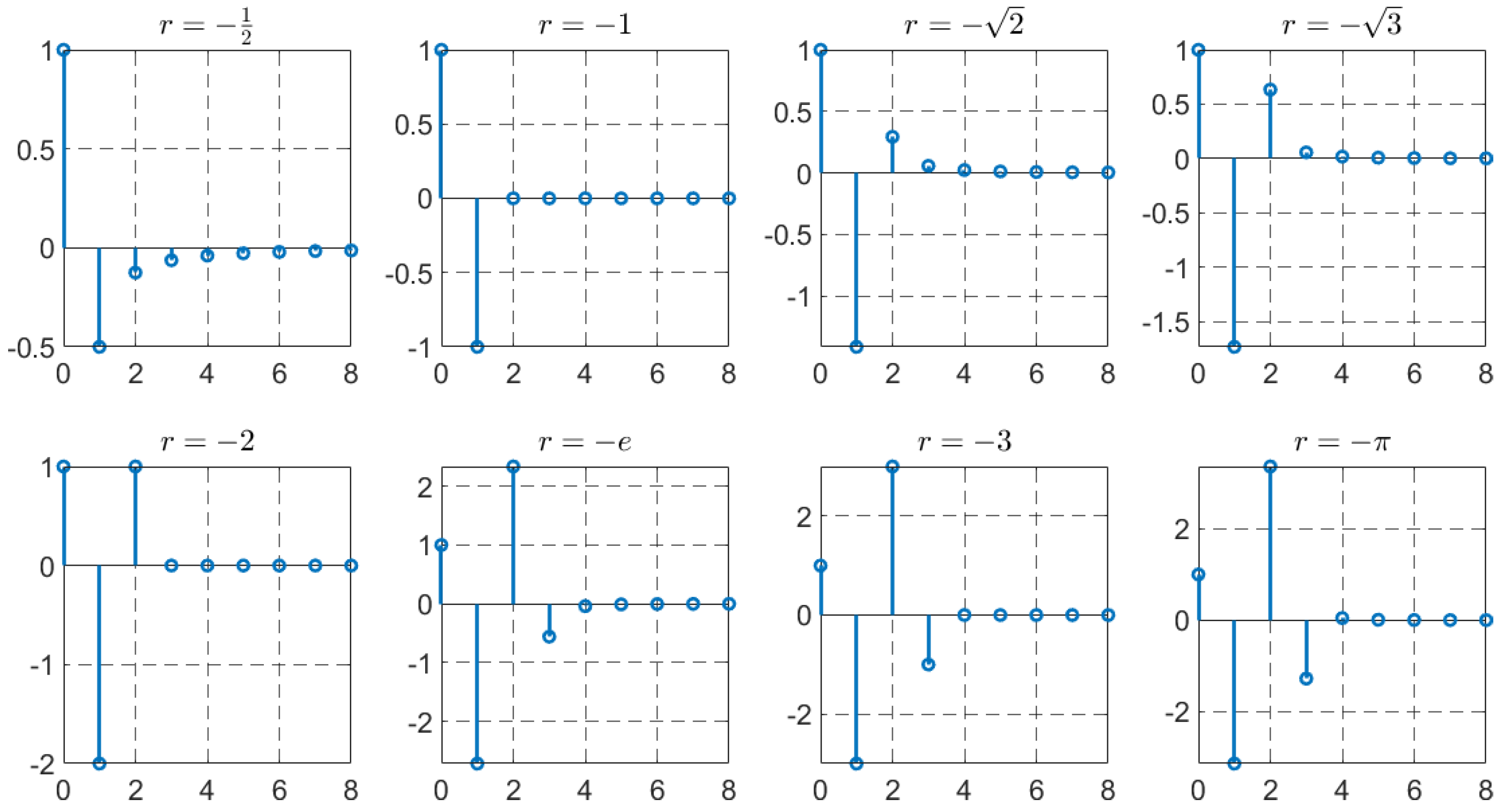
Figure 2.
Accumulative convolution sequences with inverse fractional -th order.

Figure 3.
Convolution results of with different r-th order. The first and third * on the superscript represent the exponentiated convolution, and the second * represents the convolution operation.
Figure 3.
Convolution results of with different r-th order. The first and third * on the superscript represent the exponentiated convolution, and the second * represents the convolution operation.

Figure 4.
Cobweb-diagram of 19 Lorenz iterations with the initial condition . One colour represents one step of the iteration process.
Figure 4.
Cobweb-diagram of 19 Lorenz iterations with the initial condition . One colour represents one step of the iteration process.

Figure 5.
The sequence obtained from the Lorenz iterations.

Figure 6.
Data transformation—absolute values of the Lorenz iteration sequence.

Figure 7.
Data transformation—first-order accumulative absolute values by convolution. The first * represents the convolution operation, and the second * on the superscript represents the exponentiated convolution.
Figure 7.
Data transformation—first-order accumulative absolute values by convolution. The first * represents the convolution operation, and the second * on the superscript represents the exponentiated convolution.

Figure 8.
Comparison of fitted results from different orders.

Figure 9.
MAPE curve with respect to the accumulative convolution order r.

Figure 10.
Comparison of the original sequence “hr.207” and the fitted results from the GM(1,1) model.
Figure 10.
Comparison of the original sequence “hr.207” and the fitted results from the GM(1,1) model.

Figure 11.
APE of the original sequence “hr.207” using the GM(1,1) model.

Figure 12.
MAPE of the original sequence “hr.207” using the GM(1,1) model.

Figure 13.
Comparison of the original sequence “hr.237” and the fitted results from the GM(1,1) model.
Figure 13.
Comparison of the original sequence “hr.237” and the fitted results from the GM(1,1) model.

Figure 14.
APE of the original sequence “hr.237” using the GM(1,1) model.

Figure 15.
APE of the original sequence “hr.237” using the GM(1,1) model.

Figure 16.
Comparison of the original sequence “hr.11839” and the fitted results from the GM(1,1) model.
Figure 16.
Comparison of the original sequence “hr.11839” and the fitted results from the GM(1,1) model.

Figure 17.
APE of the original sequence “hr.11839” using the GM(1,1) model.

Figure 18.
MAPE of the original sequence “hr.11839” using the GM(1,1) model.

Figure 19.
Comparison of the original sequence “hr.7257” and the fitted results from the GM(1,1) model.
Figure 19.
Comparison of the original sequence “hr.7257” and the fitted results from the GM(1,1) model.

Figure 20.
APE of original sequence “hr.7257” by GM(1,1) model.

Figure 21.
MAPE of the original sequence “hr.7257” using the GM(1,1) model.


Table 1.
Accumulative convolution sequences with fractional r-th order.
| r | 1 | 2 | e | 3 | |||||
|---|---|---|---|---|---|---|---|---|---|
| n | |||||||||
| 0 | 1.000 | 1.000 | 1.000 | 1.000 | 1.000 | 1.000 | 1.000 | 1.000 | |
| 1 | 0.500 | 1.000 | 1.414 | 1.732 | 2.000 | 2.718 | 3.000 | 3.142 | |
| 2 | 0.375 | 1.000 | 1.707 | 2.366 | 3.000 | 5.054 | 6.000 | 6.506 | |
| 3 | 0.313 | 1.000 | 1.943 | 2.943 | 4.000 | 7.948 | 10.000 | 11.150 | |
| 4 | 0.273 | 1.000 | 2.144 | 3.482 | 5.000 | 11.363 | 15.000 | 17.119 | |
| 5 | 0.246 | 1.000 | 2.322 | 3.992 | 6.000 | 15.267 | 21.000 | 24.452 | |
| 6 | 0.226 | 1.000 | 2.482 | 4.479 | 7.000 | 19.640 | 28.000 | 33.179 | |
| 7 | 0.209 | 1.000 | 2.629 | 4.947 | 8.000 | 24.461 | 36.000 | 43.330 | |
| 8 | 0.196 | 1.000 | 2.765 | 5.400 | 9.000 | 29.714 | 45.000 | 54.930 | |
Table 2.
Accumulative convolution sequences with inverse fractional -th order.
| r | |||||||||
|---|---|---|---|---|---|---|---|---|---|
| n | |||||||||
| 0 | 1.0000 | 1 | 1.0000 | 1.0000 | 1 | 1.0000 | 1 | 1.0000 | |
| 1 | −0.5000 | −1 | −1.4142 | −1.7321 | −2 | −2.7183 | −3 | −3.1416 | |
| 2 | −0.1250 | 0 | 0.2929 | 0.6340 | 1 | 2.3354 | 3 | 3.3640 | |
| 3 | −0.0625 | 0 | 0.0572 | 0.0566 | 0 | −0.5592 | −1 | −1.2801 | |
| 4 | −0.0391 | 0 | 0.0227 | 0.0179 | 0 | −0.0394 | 0 | 0.0453 | |
| 5 | −0.0273 | 0 | 0.0117 | 0.0081 | 0 | −0.0101 | 0 | 0.0078 | |
| 6 | −0.0205 | 0 | 0.0070 | 0.0044 | 0 | −0.0038 | 0 | 0.0024 | |
| 7 | −0.0161 | 0 | 0.0046 | 0.0027 | 0 | −0.0018 | 0 | 0.0010 | |
| 8 | −0.0131 | 0 | 0.0032 | 0.0018 | 0 | −0.0010 | 0 | 0.0005 | |
Table 3.
Comparison of the fitted results from different order GM(1,1) models.
| n | GM | GM | GM | |
|---|---|---|---|---|
| 0 | 0.1550 | 0.1550 | 0.1550 | 0.1550 |
| 1 | 1.1069 | 2.2874 | 1.2752 | 1.1070 |
| 2 | 1.9194 | 2.5438 | 1.9276 | 1.7767 |
| 3 | 2.2394 | 2.8290 | 2.4809 | 2.3684 |
| 4 | 3.0346 | 3.1461 | 2.9973 | 2.9264 |
| 5 | 3.2991 | 3.4988 | 3.5005 | 3.4690 |
| 6 | 4.1591 | 3.8910 | 4.0029 | 4.0062 |
| 7 | 4.6386 | 4.3272 | 4.5122 | 4.5444 |
| 8 | 5.1788 | 4.8122 | 5.0339 | 5.0878 |
| 9 | 5.5951 | 5.3517 | 5.5721 | 5.6399 |
| 10 | 6.2485 | 5.9516 | 6.1304 | 6.2032 |
| 11 | 6.3946 | 6.6187 | 6.7118 | 6.7801 |
| 12 | 7.3519 | 7.3607 | 7.3193 | 7.3724 |
| 13 | 8.1848 | 8.1858 | 7.9556 | 7.9820 |
| 14 | 8.5722 | 9.1034 | 8.6234 | 8.6105 |
| 15 | 9.2721 | 10.1239 | 9.3253 | 9.2596 |
| MAPE | in-sample | 13.9748% | 3.4191% | 2.5166% |
| 16 | 9.2923 | 11.2587 | 10.0642 | 9.9308 |
| 17 | 10.2915 | 12.5208 | 10.8427 | 10.6256 |
| 18 | 11.2882 | 13.9244 | 11.6639 | 11.3454 |
| MAPE | out-of-sample | 22.0589% | 5.6635% | 3.5414% |
Disclaimer/Publisher’s Note: The statements, opinions and data contained in all publications are solely those of the individual author(s) and contributor(s) and not of MDPI and/or the editor(s). MDPI and/or the editor(s) disclaim responsibility for any injury to people or property resulting from any ideas, methods, instructions or products referred to in the content. |
© 2023 by the author. Licensee MDPI, Basel, Switzerland. This article is an open access article distributed under the terms and conditions of the Creative Commons Attribution (CC BY) license (https://creativecommons.org/licenses/by/4.0/).
Share and Cite
MDPI and ACS Style
Chen, T. Fractional-Order Accumulative Generation with Discrete Convolution Transformation. Fractal Fract. 2023, 7, 402. https://doi.org/10.3390/fractalfract7050402
AMA Style
Chen T. Fractional-Order Accumulative Generation with Discrete Convolution Transformation. Fractal and Fractional. 2023; 7(5):402. https://doi.org/10.3390/fractalfract7050402
Chicago/Turabian StyleChen, Tao. 2023. "Fractional-Order Accumulative Generation with Discrete Convolution Transformation" Fractal and Fractional 7, no. 5: 402. https://doi.org/10.3390/fractalfract7050402