Subordination Principle for Generalized Fractional Zener Models

Abstract

The fractional Zener constitutive law is frequently used as a model of solid-like viscoelastic behavior. In this work, a class of linear viscoelastic models of Zener type, which generalize the fractional Zener model, is studied by the use of Bernstein functions technique. We prove that the corresponding relaxation moduli are completely monotone functions under appropriate thermodynamic restrictions on the parameters. Based on this property, we study the propagation function and establish the subordination principle for the corresponding Zener-type wave equation, which provides an integral representation of the solution in terms of the propagation function and the solution of a related classical wave equation. The analytical findings are supported by numerical examples.

1. Introduction

The application of fractional derivatives in time in rheological constitutive equations has a long history [1]. One of the advantages of fractional time-derivatives in linear viscoelasticity is that with their help the damping behavior of viscoelastic media is described by using less parameters, compared with integer-order models. For a review of the main aspects of wave propagation in linear homogeneous viscoelastic media and the simplest and most used fractional constitutive models, we refer to [2].

In linear viscoelasticity, the rheological properties of a viscoelastic medium are described through a linear constitutive relation between stress $\sigma$ and strain $\epsilon$. Following [2], we restrict our considerations to the uniaxial case, in which $\sigma =\sigma (x,t)$ and $\epsilon =\epsilon (x,t)$, and consider systems quiescent for all times prior to some starting time $t=0$.

The fractional Zener constitutive law is extensively used as a model of solid-like viscoelastic behavior [2,3]. The fractional Zener stress–strain relation reads

$$(1+a{D}_t^{\alpha })\sigma (x,t)=(1+b{D}_t^{\alpha })\epsilon (x,t),$$

(1)

where $D_t^{\alpha }$ denotes the Riemann–Liouville fractional derivative [4] of order $\alpha \in (0,1)$ and $a>0,b>0$. Constitutive Equation (1) is introduced for the first time in 1971 by Caputo and Mainardi [5,6]. Another early extensive study of model (1) can be found in [7]. A necessary and sufficient condition for physical acceptability of model (1) is the restriction $a\le b$. Under this condition, the corresponding relaxation modulus is a completely monotone function, see, e.g., [2].

Recall that a functions $f\left(t\right)$ is said to be completely monotone if it is real-valued and infinitely differentiable on ${\mathbb{R}}_{+}$ and

$${(-1)}^n{f}^{\left(n\right)}\left(t\right)\ge 0,t>0,n=0,1,2,\dots$$

(2)

Completely monotonic relaxation moduli are commonly encountered in polymer physics and other branches of rheology and mechanics [2,8,9]. For a discussion on the importance of the complete monotonicity property of the relaxation moduli in linear viscoelasticity, we refer to [9].

Wave equations in viscoelastic media described by the fractional Zener model are studied in many works, see, e.g., [3,10] and the references cited there. Various types of distributed-order generalizations of model (1) are proposed and studied along with the corresponding wave equations: see, e.g., [11,12,13,14,15,16]. The complete monotonicity of the relaxation modulus for Zener-type constitutive equations with multiple time-derivatives and distributed-order time-derivatives with power-type weight function is established in [17] under appropriate constraints on the parameters. The proofs are based on a representation of the relaxation modulus as a Laplace transform of a non-negative spectral function. For other applications of this method, we refer to [2,18].

Recently, equations with general fractional differential operators have gained increasing interest, see the pioneering work [19], the review [20], as well as [21,22,23,24,25], to mention only few of many publications from the last years.

In the article [26], published very recently, a generalization of model (1) in the context of general fractional calculus is proposed and studied. In this work, the fractional derivative $D_t^{\alpha }$ in the constitutive Equation (1) is replaced by a general convolutional derivative. For two specific cases of the kernel of this derivative, it is proven that the condition $a<b$ is sufficient for the dissipation inequality to hold and thus, for the thermodynamic compatibility of the corresponding viscoelastic models.

Motivated by the work [26], in the present paper, we study the following generalized fractional Zener model

$$\left(1+a{D}_t^{\left(k\right)}\right)\sigma (x,t)=\left(1+b{D}_t^{\left(k\right)}\right)\epsilon (x,t).$$

(3)

Here, $a>0$ and $b>0$ are given parameters, and $D_t^{\left(k\right)}$ is a generalized convolutional derivative in the Riemann–Liouville sense, defined by

$$\left(D_t^{\left(k\right)}f\right)\left(t\right)=\frac{\mathrm{d}}{\mathrm{d}t}{\int }_0^{t}k(t-\tau )f\left(\tau \right)\mathrm{d}\tau ,t>0,$$

(4)

where k is a locally integrable memory kernel, $k\in L_{loc}^1\left({\mathbb{R}}_{+}\right)$. For the kernel $k\left(t\right)$, we assume in addition that its Laplace transform $\widehat{k}\left(s\right)$ exists for all $s>0$ and

$$\widehat{k}\left(s\right)\in \mathcal{SF},\underset{s\to +\infty }{lim}s\widehat{k}\left(s\right)=+\infty ,$$

(5)

where $\mathcal{SF}$ denotes the class of Stieltjes functions. The precise definition of this class is given in the next section, see (6). The basic particular examples of operators $D_t^{\left(k\right)}$, defined in this way, are the first-order derivative (in this case, $\widehat{k}\left(s\right)=1$), the Riemann–Liouville fractional derivative of order $\alpha \in (0,1)$ (corresponding to $\widehat{k}\left(s\right)=s^{\alpha -1}$), as well as linear combinations with positive coefficients of such derivatives.

Let us note that assumptions (5) are slightly weaker than those required in the definition of the general fractional derivative, introduced in [19] and studied in detail in [20,22], where additional assumptions on the limiting behavior of $\widehat{k}\left(s\right)$ are imposed. We also point out that the assumption $\widehat{k}\left(s\right)\in \mathcal{SF}$, which is essential also in the definition of the general fractional derivative in [19], allows the use of the convenient Bernstein functions technique developed in [27].

In this work, based on the Bernstein functions technique, we establish the complete monotonicity of the relaxation modulus for model (3), provided the constraint $a\le b$ is satisfied. This result is stronger than the thermodynamic compatibility results proven in [26], since the dissipation inequality is satisfied for systems with completely monotone relaxation moduli. The complete monotonicity property implies also the subordination principle for the generalized fractional Zener wave equation. The propagation function is obtained as the solution of an equation governing wave propagation in a viscoelastic half-space with the generalized fractional Zener model (3) and its properties are studied. The relation between the propagation function and the subordination kernel is established. Some examples of application of subordination principle are given. Numerical results for specific cases of generalized derivatives are presented and discussed.

The rest of the paper is organized as follows. Section 2 contains preliminaries and properties of Bernstein functions and related classes of functions, which are necessary for the study. In Section 3, we establish the complete monotonicity property of the relaxation modulus and discuss the relation of this property with thermodynamic compatibility conditions. Propagation of waves in generalized fractional Zener medium is discussed in Section 4. A subordination principle is formulated in Section 5 and applied to two basic problems. Numerical examples for some specific kernels are discussed in Section 6. The last Section 7 contains concluding remarks.

2. Preliminaries

This section contains preliminaries on the following functions classes: completely monotone functions ($\mathcal{CMF}$), Stieltjes functions ($\mathcal{SF}$), Bernstein functions ($\mathcal{BF}$) and complete Bernstein function ($\mathcal{CBF}$). Their definitions and properties, necessary for our proofs, are given in the terminology of [27].

We use the following notations for the Laplace transform of a function

$$\mathcal{L}\left\{f\left(t\right)\right\}\left(s\right)=\widehat{f}\left(s\right)={\int }_0^{\infty }{e}^{-st}f\left(t\right)\mathrm{d}t.$$

The Laplace transform of a function $u(x,t)$ with respect to the time variable t, where x is considered as a parameter, is denoted by $\widehat{u}(x,s)$ or $\mathcal{L}\left\{u\right\}(x,s)$.

We proceed with the definitions of the four special classes of functions. The definition of the class $\mathcal{CMF}$ of completely monotone functions is already given in the Section 1, see (2). The characterization of the class $\mathcal{CMF}$ is given by the Bernstein’s theorem: a function is completely monotone if and only if it can be represented as the Laplace transform of a non-negative (generalized) function.

The class $\mathcal{BF}$ of Bernstein functions consists of all non-negative functions $f\left(t\right)$ defined and infinitely differentiable on ${\mathbb{R}}_{+}$, such that $f^{\prime }\left(t\right)\in \mathcal{CMF}.$

The class of Stieltjes functions ($\mathcal{SF}$) consists of all functions $\phi$ defined on ${\mathbb{R}}_{+}$ which admit the representation (see [19])

$$\phi \left(s\right)={\phi }_0+{\int }_0^{\infty }{e}^{-s\tau }f\left(\tau \right)d\tau ,s>0,$$

(6)

where ${\phi }_0\ge 0$, $f\in \mathcal{CMF}\cap L_{loc}^1\left({\mathbb{R}}_{+}\right)$, and the Laplace transform of f exists for any $s>0$. The constant ${\phi }_0$ can be determined from the identity (see, e.g., [28], Theorem 2.6) ${\phi }_0={lim}_{s\to +\infty }\phi \left(s\right)$.

The class $\mathcal{CBF}$ of complete Bernstein functions consists of all function $\phi$ defined on ${\mathbb{R}}_{+}$, such that $\phi \left(s\right)/s\in \mathcal{SF},s>0.$

The simplest examples of functions from the classes $\mathcal{CBF}$ and $\mathcal{SF}$ are given as:

$$\mathrm{if} \alpha \in [0,1] \mathrm{then} s^{\alpha }\in \mathcal{CBF} \mathrm{and} s^{-\alpha }\in \mathcal{SF}.$$

(7)

The following properties are satisfied for $s>0$:

(P1)

The set $\mathcal{CMF}$ is a convex cone: ${\lambda }_1{f}_1+{\lambda }_2{f}_2\in \mathcal{CMF}$ for all $f_1,f_2\in \mathcal{CMF}$ and ${\lambda }_1,{\lambda }_2\ge 0$. Moreover, $f_1·f_2\in \mathcal{CMF}$ for all $f_1,f_2\in \mathcal{CMF}$. The set $\mathcal{CMF}$ is closed under pointwise limits;

(P2)

The sets $\mathcal{SF}$, $\mathcal{BF}$ and $\mathcal{CBF}$ are convex cones. They are closed under pointwise limits;

(P3)

Any Stieltjes function is completely monotone. Any complete Bernstein function is a Bernstein function;

(P4)

Let $\phi \in \mathcal{BF}$. Then, the function $\phi \left(s\right)/s$ is completely monotone;

(P5)

$\mathcal{CMF}\circ \mathcal{BF}\subset \mathcal{CMF}$, where ∘ denotes composition of functions from the corresponding sets;

(P6)

Every function $\phi \in \mathcal{SF}$, such that ${lim}_{s\to +\infty }\phi \left(s\right)=0$, is the Laplace transform of a function $f\left(t\right)$, which is locally integrable on ${\mathbb{R}}_{+}$ and completely monotone;

(P7)

$\phi \in \mathcal{SF}$ if and only if $s\phi \left(s\right)\in \mathcal{CBF}$;

(P8)

Let $\phi \ne 0$. Then, $\phi \left(s\right)\in \mathcal{CBF}$ if and only if ${\left(\phi \left(s\right)\right)}^{-1}\in \mathcal{SF}$;

(P9)

Let $\phi ,\psi \in \mathcal{CBF}$. Assume ${\mu }_1,{\mu }_2\in (0,1)$ are such that ${\mu }_1+{\mu }_2\le 1$. Then,

$${\phi }^{{\mu }_1}\left(s\right)·{\psi }^{{\mu }_2}\left(s\right)\in \mathcal{CBF};$$

(P10)

Any function $\phi$ from the sets $\mathcal{CBF}$ or $\mathcal{SF}$ admits an analytic extension to the complex plane cut along the negative real axis $\mathbb{C}\backslash (-\infty ,0]$, which satisfies

$$|arg\phi (z\left)\right|\le |argz|,z\in \mathbb{C}\backslash (-\infty ,0].$$

Moreover, ${\left(\phi \left(z\right)\right)}^{*}=\phi \left(z^{*}\right)$, where * denotes the complex conjugate, and

$$\Im \phi \left(z\right)·\Im z\le 0\mathrm{for}\phi \in \mathcal{SF};\Im \phi \left(z\right)·\Im z\ge 0\mathrm{for}\phi \in \mathcal{CBF}.$$

For details on the proofs, see [27,28], Theorem 2.6.

The Mittag–Leffler function is defined as follows:

$$E_{\alpha ,\beta }\left(z\right)=\sum _{k=0}^{\infty }\frac{z^k}{\mathrm{\Gamma }(\alpha k+\beta )},$$

(8)

where $\alpha >0,\beta \in \mathbb{R}$ and $z\in \mathbb{C}$. If $\lambda >0$ and $0<\alpha \le \beta \le 1$, then the function of Mittag–Leffler type $t^{\beta -1}{E}_{\alpha ,\beta }(-\lambda t^{\alpha })$ is completely monotone for $t>0$. The Laplace transform of this function is given by the identity

$$\mathcal{L}\left\{t^{\beta -1}{E}_{\alpha ,\beta }(-\lambda t^{\alpha })\right\}\left(s\right)=\frac{s^{\alpha -\beta }}{s^{\alpha }+\lambda },t>0.$$

(9)

3. Completely Monotone Relaxation Modulus

Consider the generalized Zener constitutive Equation (3). We assume that $\epsilon (x,t)=0$ and $\sigma (x,t)=0$ for all $x\in \mathbb{R}$ and $t<0$. Moreover, we suppose that $\epsilon \in C^1\left({\mathbb{R}}_{+}\right)$.

Let us note that the assumption $\widehat{k}\left(s\right)\in \mathcal{SF}$ is equivalent to the following representation of the kernel $k\left(t\right)$

$$k\left(t\right)=k_0\delta \left(t\right)+k_1\left(t\right),$$

(10)

where $k_0\ge 0$, $\delta (·)$ denotes the Dirac delta function and $k_1\left(t\right)\in L_{loc}^1\left({\mathbb{R}}_{+}\right)$ is a completely monotone function.

The relaxation modulus $G\left(t\right)$ in a linear viscoelastic model is defined as the stress response to a unit step of strain. Specifically, for a quiescent system at $t=0$, the following equation is satisfied [2]:

$$\sigma (x,t)={\int }_0^{t}G(t-\tau )\frac{\partial \epsilon }{\partial \tau }(x,\tau )\mathrm{d}\tau .$$

(11)

Applying formally the Laplace transform to (3) and taking into account the Laplace transform identity $\mathcal{L}\left\{D_t^{\left(k\right)}u\right\}\left(s\right)=s\widehat{k}\left(s\right)$, we deduce

$$\left(1+as\widehat{k}\left(s\right)\right)\widehat{\sigma }(x,s)=\left(1+bs\widehat{k}\left(s\right)\right)\widehat{\epsilon }(x,s).$$

This, together with the identity $\widehat{\sigma }(x,s)=\widehat{G}\left(s\right)s\widehat{\epsilon }(x,s)$ (which follows from (11)), yields

$$\widehat{G}\left(s\right)=\frac{1+bs\widehat{k}\left(s\right)}{s(1+as\widehat{k}\left(s\right))}.$$

(12)

We next discuss the properties of the relaxation modulus $G\left(t\right)$, based on the Laplace transform pair (12).

In a thermodynamically compatible model, the function $G\left(t\right)$ is non-negative and non-increasing. We prove next that these properties can be satisfied only if $a\le b$. Indeed, since the rate of relaxation is non-increasing, $G^{\prime }\left(t\right)\le 0$, it follows $\mathcal{L}\left\{G^{\prime }\right\}\left(s\right)\le 0$ for $s>0$. Therefore, taking into account identity (12), we obtain for $s>0$

$$\mathcal{L}\left\{\frac{\mathrm{d}G}{\mathrm{d}t}\right\}\left(s\right)=s\widehat{G}\left(s\right)-\underset{t\to 0^{+}}{lim}G\left(t\right)=\frac{1+bs\widehat{k}\left(s\right)}{1+as\widehat{k}\left(s\right)}-\frac{b}{a}=\frac{a-b}{a(1+as\widehat{k}\left(s\right))}\le 0.$$

(13)

Here, we have used that the initial value theorem for the Laplace transform implies

$$\underset{t\to 0^{+}}{lim}G\left(t\right)=\underset{s\to +\infty }{lim}s\widehat{G}\left(s\right)=\underset{s\to +\infty }{lim}\frac{1+bs\widehat{k}\left(s\right)}{1+as\widehat{k}\left(s\right)}=\frac{b}{a}$$

(14)

due to the assumption $s\widehat{k}\left(s\right)\to +\infty$ as $s\to +\infty$. The inequality in (13) implies $a\le b$, since the denominator is a positive function. In this way, we have proved that condition $a\le b$ is necessary for viscoelastic model (3) to be physically acceptable.

We prove next that the restriction $a\le b$ together with the assumptions (5) on the kernel $k\left(t\right)$ implies the complete monotonicity of the relaxation modulus for viscoelastic model (3).

Theorem 1.

Assume that $0<a\le b$ and that conditions (5) on the kernel $k\left(t\right)$ are satisfied. Then, there exists a locally integrable and completely monotone function $G\left(t\right)$, $t\ge 0$, which Laplace transform is given by the identity (12).

Proof. 

For the proof, we use the Bernstein functions technique. For $s>0$, it holds

$$s\widehat{G}\left(s\right)=\frac{1+bs\widehat{k}\left(s\right)}{1+as\widehat{k}\left(s\right)}=1+(b-a)\frac{1}{{\left(s\widehat{k}\left(s\right)\right)}^{-1}+a}\in \mathcal{CBF}.$$

(15)

Here, we use the assumption $\widehat{k}\left(s\right)\in \mathcal{SF}$, which is equivalent to ${\left(s\widehat{k}\left(s\right)\right)}^{-1}\in \mathcal{SF}$ (see properties (P7) and (P8)). Since $a>0$, this implies ${\left(s\widehat{k}\left(s\right)\right)}^{-1}+a\in \mathcal{SF}$. By (P8), this is equivalent to ${\left({\left(s\widehat{k}\left(s\right)\right)}^{-1}+a\right)}^{-1}\in \mathcal{CBF}$, which, by noting that $b-a\ge 0$, yields $s\widehat{G}\left(s\right)\in \mathcal{CBF}$. Applying again (P7), it follows $\widehat{G}\left(s\right)\in \mathcal{SF}$. Moreover, (12) and assumption $s\widehat{k}\left(s\right)\to +\infty$ as $s\to +\infty$ imply ${lim}_{s\to +\infty }\widehat{G}\left(s\right)=0$. Therefore, according to (P6), there exists a locally integrable function $G\left(t\right)\in \mathcal{CMF}$, which Laplace transform is given by (12). □

By the uniqueness of Laplace transform, it follows that the function $G\left(t\right)$ from the above theorem coincides with the relaxation modulus of constitutive model (3). In this way, we proved that the generalized Zener constitutive Equation (3) defines a viscoelastic system with a completely monotonic relaxation modulus. It is known (see, e.g., [8]) that systems with completely monotonic relaxation moduli obey the dissipation inequality, that is, for any $x\in \mathbb{R}$ and $T>0$, the following holds:

$${\int }_0^T\sigma (x,t)\frac{\partial \epsilon }{\partial t}(x,t)\mathrm{d}t\ge 0.$$

(16)

Corollary 1.

Under the conditions of Theorem 1, the dissipation inequality (16) is satisfied for model (3).

Proof. 

For completeness, we give a direct proof of (16). Taking into account (11), the dissipation inequality (16) is equivalent to

$${\int }_0^T\left({\int }_0^{t}G(t-\tau )\frac{\partial \epsilon }{\partial \tau }(x,\tau )\mathrm{d}\tau \right)\frac{\partial \epsilon }{\partial t}(x,t)\mathrm{d}t\ge 0.$$

(17)

This is satisfied when $G\left(t\right)$ is a function of positive type, that is,

$${\int }_0^T\left({\int }_0^{t}G(t-\tau )u(x,\tau )d\tau \right)u(x,t)\mathrm{d}t\ge 0\mathrm{for}\mathrm{every}u\in L^2(0,T).$$

(18)

We will use the fact that every completely positive function is a function of positive type, see, e.g., [29], Theorem 3.1. A function $G\left(t\right)$ is called completely positive if it satisfies the following conditions: $G\in L^1(0,T)$ and there exist $\gamma \ge 0$ and a non-negative and non-increasing function $K\in L^1(0,T)$, such that

$$\gamma G\left(t\right)+{\int }_0^{t}K(t-\tau )G\left(\tau \right)\mathrm{d}\tau =1,t\in [0,T].$$

(19)

It is known that any completely monotone function is completely positive, see, e.g., [29]. For completeness, we will check directly that the relaxation modulus $G\left(t\right)$ for the generalized Zener model (3) is a completely positive function. To this end, let us consider the function

$$F\left(s\right)=\frac{b-a}{b(1+bs\widehat{k}\left(s\right))},s>0.$$

Since $s\widehat{k}\left(s\right)$ is a complete Bernstein function and $b-a\ge 0$, property (P8) implies $F\left(s\right)\in \mathcal{SF}$. Moreover, ${lim}_{s\to \infty }F\left(s\right)=0$. Therefore, according to (P6), there exists a locally integrable function $K\left(t\right)\in \mathcal{CMF}$, such that $\widehat{K}\left(s\right)=F\left(s\right)$. Then, identity (19) is satisfied with $K\left(t\right)$ defined in this way and $\gamma =a/b$. This can be easily checked by applying Laplace transform since

$$\gamma \widehat{G}\left(s\right)+\widehat{K}\left(s\right)\widehat{G}\left(s\right)=1/s.$$

Therefore, the dissipation inequality (16) is satisfied for model (3). □

Let us note that conditions for thermodynamic compatibility are considered in different form in [7]. In our notation, these conditions read

$$\Re \left\{\mathrm{i}\omega \widehat{G}\left(\mathrm{i}\omega \right)\right\}\ge 0,\Im \left\{\mathrm{i}\omega \widehat{G}\left(\mathrm{i}\omega \right)\right\}\ge 0,\forall \omega >0.$$

(20)

For completely monotone functions $G\left(t\right)$, conditions (20) are always fulfilled. This follows from the fact that in this case, $\widehat{G}\left(s\right)\in \mathcal{SF}$, which is equivalent to $s\widehat{G}\left(s\right)\in \mathcal{CBF}$ (see (P7)), and then properties (P10) imply (20).

Let us point out that since $s\widehat{k}\left(s\right)\in \mathcal{CBF}$, the limit ${lim}_{s\to 0^{+}}s\widehat{k}\left(s\right)$ exists and is real (see [27], Theorem 6.2), which implies

$$\underset{t\to +\infty }{lim}G\left(t\right)=\underset{s\to 0^{+}}{lim}s\widehat{G}\left(s\right)=\underset{s\to 0^{+}}{lim}\frac{1+bs\widehat{k}\left(s\right)}{1+as\widehat{k}\left(s\right)}>0.$$

(21)

This limit confirms that the class of models (3) govern solid-like behavior, see, e.g., [2].

4. Generalized Fractional Zener Wave Equation

The one-dimensional equation governing wave propagation in a viscoelastic medium with the generalized Zener constitutive law is derived by combining constitutive Equation (3), the one-dimensional equation of motion

$$\frac{\partial }{\partial x}\sigma (x,t)+f(x,t)=\frac{{\partial }^2}{\partial t^2}u(x,t)$$

(22)

and the kinematic equation

$$\epsilon (x,t)=\frac{\partial }{\partial x}u(x,t),$$

(23)

where $u(x,t)$ denotes the particle displacement, $f(x,t)$ is the body force, $x\in \mathbb{R}$, and $t>0$. Combining the three equations, we derive formally the following generalized wave equation of Zener type

$$\left(1+a{D}_t^{\left(k\right)}\right)\frac{{\partial }^2}{\partial t^2}u(x,t)=\left(1+b{D}_t^{\left(k\right)}\right)\frac{{\partial }^2}{\partial x^2}u(x,t)+\left(1+a{D}_t^{\left(k\right)}\right)f(x,t).$$

(24)

It is worth noting that in the limiting case $a=b$, Equation (24) is the classical wave equation, which is well studied. Therefore, in what follows, we consider only coefficients satisfying

$$0<a<b.$$

Assuming the initial conditions

$$\underset{t\to 0^{+}}{lim}u(x,t)=v\left(x\right)\mathrm{and}\underset{t\to 0^{+}}{lim}\frac{\partial }{\partial t}u(x,t)=0,$$

(25)

we rewrite the wave Equation (24) as a Volterra integral equation as follows. Applying Laplace transform to (24) and taking into account the initial conditions (25), we obtain

$$\widehat{u}(x,s)=v\left(x\right)\frac{1}{s}+\frac{1+bs\widehat{k}\left(s\right)}{s^2(1+as\widehat{k}\left(s\right))}\mathcal{L}\left\{\frac{{\partial }^{2}u}{\partial x^2}\right\}(x,s)+\frac{1}{s^2}\widehat{f}(x,s).$$

(26)

Denote by $\xi \left(t\right)$ the function with Laplace transform

$$\widehat{\xi }\left(s\right)=\frac{1+bs\widehat{k}\left(s\right)}{s^2(1+as\widehat{k}\left(s\right))}.$$

According to (12), the function $\xi \left(t\right)$ is well defined and

$$\xi \left(t\right)={\int }_0^{t}G\left(\tau \right)\mathrm{d}\tau ,t\ge 0.$$

(27)

Taking the inverse Laplace transform in (26), we derive the following Volterra integral equation

$$u(x,t)=v\left(x\right)+{\int }_0^t\xi (t-\tau )\frac{{\partial }^2}{\partial x^2}u(x,\tau )\mathrm{d}\tau +h(x,t),$$

(28)

where $h(x,t)={\int }_0^t(t-\tau )f(x,\tau )\mathrm{d}\tau .$ Let us note that $G\left(t\right)\in \mathcal{CMF}$ implies $\xi \left(t\right)\in \mathcal{BF}.$

In what follows, we study Equation (28) as a model for wave propagation in a viscoelastic medium with the generalized Zener constitutive law (3). We consider different possibilities for the domain of the spatial operator.

4.1. Propagation Function

Let us consider first the basic problem of wave propagation of impact waves in a viscoelastic half-space with constitutive Equation (3):

$$\begin{array}{ccc}& & w(x,t)={\int }_0^t\xi (t-\tau )\frac{{\partial }^2}{\partial x^2}w(x,\tau )\mathrm{d}\tau ,x,t>0,\hfill \end{array}$$

(29)

$$\begin{array}{ccc}& & w(0,t)=H\left(t\right),w\to 0\mathrm{a}sx\to \infty ,t>0,\hfill \end{array}$$

(30)

where the kernel $\xi$ is defined in (27) and $H\left(t\right)$ is the Heaviside unit step function. The solution $w(x,t)$ is often referred to as propagation function, since it represents the propagation in time of a disturbance at $x=0$.

It is worth noting that in the limiting case $a=b$, corresponding to the classical wave equation, the propagation function is $w(x,t)=H(t-x)$.

Let us also note that the initial conditions

$$\underset{t\to 0^{+}}{lim}w(x,t)=\underset{t\to 0^{+}}{lim}\frac{\partial }{\partial t}w(x,t)=0,$$

(31)

follow from Equation (29), taking into account representation (27) for the kernel $\xi \left(t\right)$.

By applying Laplace transform with respect to the temporal variable in (29) and (30), we obtain the following ODE in x (with s considered as a parameter):

$$g\left(s\right)\widehat{w}(x,s)=\frac{{\partial }^2\widehat{w}}{\partial x^2}(x,s),\widehat{w}(0,s)=1/s,\widehat{w}(x,s)\to 0\mathrm{a}sx\to \infty ,$$

(32)

where

$$g\left(s\right)=\frac{1}{\widehat{\xi }\left(s\right)}=s^2\frac{1+as\widehat{k}\left(s\right)}{1+bs\widehat{k}\left(s\right)}.$$

(33)

The solution of problem (32) is given by

$$\widehat{w}(x,s)=\frac{1}{s}exp\left(-x\sqrt{g\left(s\right)}\right).$$

(34)

The following property is important in the study of the behavior of function $w(x,t)$.

Proposition 1.

If $0<a\le b$ and $k\left(t\right)$ satisfies conditions (5), then for the characteristic function $g\left(s\right)$, defined in (33), it holds

$$\sqrt{g\left(s\right)}\in \mathcal{CBF}.$$

(35)

Proof. 

Applying (33) and (12), we obtain the relation

$$g\left(s\right)=\frac{s}{\widehat{G}\left(s\right)}.$$

(36)

Since $s\in \mathcal{CBF}$ and $1/\widehat{G}\left(s\right)\in \mathcal{CBF}$ (here, we use $\widehat{G}\left(s\right)\in \mathcal{SF}$, and property (P8)), the function $g\left(s\right)$ is a product of two functions from the set $\mathcal{CBF}$. Then, (35) follows by applying property (P9) with ${\mu }_1={\mu }_2=1/2$. □

According to (35) $\sqrt{g\left(s\right)}\in \mathcal{CBF}\subset \mathcal{BF}.$ Then, property (P5) implies

$$exp\left(-x\sqrt{g\left(s\right)}\right)\in \mathcal{CMF}$$

(37)

with respect to $s>0$ (and $x>0$ considered as a parameter). Therefore, the function $\widehat{w}$ is a product of two functions, completely monotone for $s>0$, which yields $\widehat{w}(x,s)\in \mathcal{CMF}$. This implies by Bernstein’s theorem $w(x,t)\ge 0$. Moreover, the propagation function $w(x,t)$ is non-decreasing in t and non-increasing in x. This can be established in the same way as Theorem 2.2 in [30] by proving that the Laplace transforms of the functions $\partial w/\partial t$ and $-\partial w/\partial x$ are completely monotone functions. Indeed, since $1/s\in \mathcal{CMF}$, and $\sqrt{g\left(s\right)}\in \mathcal{CBF}\subset \mathcal{BF}$, by property (P4) also $\sqrt{g\left(s\right)}/s\in \mathcal{CMF}$. This, together with (37), yields

$$\mathcal{L}\left\{-\frac{\partial w}{\partial x}\right\}(x,s)=-\frac{\partial }{\partial x}\widehat{w}(x,s)=\frac{\sqrt{g\left(s\right)}}{s}exp\left(-x\sqrt{g\left(s\right)}\right)\in \mathcal{CMF}$$

as products of two completely monotone functions. Further, since ${lim}_{t\to 0^{+}}w(x,t)=0$, it follows from (34) and (37)

$$\mathcal{L}\left\{\frac{\partial w}{\partial t}\right\}(x,s)=s\widehat{w}(x,s)-\underset{t\to 0^{+}}{lim}w(x,t)=exp\left(-x\sqrt{g\left(s\right)}\right)\in \mathcal{CMF}.$$

4.2. Propagation Speed

Applying the general formula for the propagation speed c of a disturbance in a viscoelastic medium [2,31], we obtain for the considered model (3) with conditions (5)

$$c=\underset{s\to \infty }{lim}\frac{s}{\sqrt{g\left(s\right)}}=\sqrt{\frac{b}{a}}.$$

(38)

This can be seen by inverting the Laplace transform in representation (34). Therefore, the propagation speed is finite for model (3) and $w(x,t)\equiv 0$ for $x>t\sqrt{b/a}$.

From general theory (see, e.g., [31], Section 5.4) in the case of finite propagation speed c, a jump discontinuity of the propagation function $w(x,t)$ at the planar surface $x=ct$ exists only if

$$\kappa =\underset{s\to \infty }{lim}\left(\sqrt{g\left(s\right)}-s/c\right)<\infty .$$

(39)

Moreover, this discontinuity is damped exponentially with exponent $\kappa$, i.e., $w(x,t)\sim exp(-\kappa x)$ as $t\to x/c,$ and $x<ct$. In our specific case, it holds that

$$\kappa =\underset{s\to \infty }{lim}s\left[{\left(\frac{1+as\widehat{k}\left(s\right)}{1+bs\widehat{k}\left(s\right)}\right)}^{1/2}-{\left(\frac{a}{b}\right)}^{1/2}\right]=\underset{s\to \infty }{lim}{\left(\frac{a}{b}\right)}^{1/2}s\left[{\left(\frac{1+{\left(as\widehat{k}\left(s\right)\right)}^{-1}}{1+{\left(bs\widehat{k}\left(s\right)\right)}^{-1}}\right)}^{1/2}-1\right].$$

We find the leading terms in the last expression as $s\to \infty$ by taking into account the expansion ${(1+z)}^{\gamma }\sim 1+\gamma z$ as $z\to 0$, $\gamma \in \mathbb{R}$, for $z={\left(as\widehat{k}\left(s\right)\right)}^{-1}$ and $z={\left(bs\widehat{k}\left(s\right)\right)}^{-1}$. In this way, we deduce

$${\left(\frac{1+{\left(as\widehat{k}\left(s\right)\right)}^{-1}}{1+{\left(bs\widehat{k}\left(s\right)\right)}^{-1}}\right)}^{1/2}\sim 1+\frac{1}{2as\widehat{k}\left(s\right)}-\frac{1}{2bs\widehat{k}\left(s\right)},s\to \infty .$$

Therefore,

$$\kappa =\underset{s\to \infty }{lim}{\left(\frac{a}{b}\right)}^{1/2}\left(\frac{1}{a}-\frac{1}{b}\right)\frac{1}{2\widehat{k}\left(s\right)}.$$

(40)

Therefore, a jump at the wave front exists only when ${lim}_{s\to \infty }\widehat{k}\left(s\right)>0$, i.e., only when $k_0\ne 0$ in the kernel representation (10). This is, for instance, the case with the composite derivative $D_t^{\left(k\right)}=\frac{\mathrm{d}}{\mathrm{d}t}+\lambda D_t^{\alpha }$, where $D_t^{\alpha }$ denotes the Riemann–Liouville fractional derivative of order $\alpha \in (0,1)$ and $\lambda \ge 0$. For $\lambda =0$, the classical Zener model is recovered. On the other hand, if ${lim}_{s\to \infty }\widehat{k}\left(s\right)=0$ ($k_0=0$ in the kernel representation (10) and thus, $k\left(t\right)=k_1\left(t\right)\in \mathcal{CMF}$), the wave front is smooth. In this case, the coexistence of finite wave speed and absence of jump discontinuity at the wave front is observed.

In the next theorem, we summarize the most important findings in this section concerning the propagation function.

Theorem 2.

Assume that $0<a\le b$ and conditions (5) on the kernel $k\left(t\right)$ are satisfied. Then, the solution $w(x,t)$ of problem (29) and (30) is a non-negative function, non-increasing in $x\ge$ and non-decreasing in $t\ge$. Moreover, $w(x,t)\equiv 0$ for $x>t\sqrt{b/a}.$ If ${lim}_{s\to \infty }\widehat{k}\left(s\right)>0$, a jump discontinuity is observed at $x=t\sqrt{b/a}$, otherwise, the function is smooth.

Plots of the propagation functions $w(x,t)$ for specific kernels at different values of the parameters are given in Figure 1 and Figure 2. The observed behavior in the figures is in agreement with the established properties of the propagation function.

5. Subordination Principle

Subordination results for different types of generalized wave equations have been established recently, see, e.g., [30,32,33,34]. Solution representations in the context of the principle of subordination are useful, since they provide an integral decomposition of the solution of such equations in terms of the solutions of two simpler problems.

In this section, we formulate the subordination principle for equations governing wave propagation in media with the generalized Zener constitutive law (3). For the sake of generality, we formulate the results in an abstract setting, using the terminology of [31].

5.1. General Formulation

Let A be a closed operator on a Banach space X. Assume A is a generator of a strongly continuous cosine family of operators $\mathrm{Cos}\left(t\right)$. This means that the second-order abstract Cauchy problem

$$\frac{{\mathrm{d}}^{2}u}{\mathrm{d}{t}^2}=Au\left(t\right),t>0;u\left(0\right)=v\in X,\underset{t\to 0}{lim}\frac{\mathrm{d}u}{\mathrm{d}t}=0.$$

(41)

is well posed, with solution operator $\mathrm{Cos}\left(t\right)$. The Laplace transform of the cosine family $\mathrm{Cos}\left(t\right)$, generated by the operator A, is given by the identity

$${\int }_0^{\infty }{e}^{-st}\mathrm{Cos}\left(t\right)dt=s{(s^2-A)}^{-1},$$

(42)

where ${(z-A)}^{-1}$ denotes the resolvent operator of the operator A.

The problem for the abstract Volterra integral equation

$$u\left(t\right)={\int }_0^t\xi (t-\tau )Au\left(\tau \right)\mathrm{d}\tau +f\left(t\right),t>0,$$

(43)

where $\xi \in L_{loc}^1\left({\mathbb{R}}_{+}\right)$ is a scalar kernel and f-an X-valued function, is said to be well posed if and only if there exists a solution operator $S\left(t\right)$, i.e., a strongly continuous family of bounded linear operators in X which commutes with A and such that the function $u\left(t\right)=S\left(t\right)v$ satisfies the equation

$$u\left(t\right)=v+{\int }_0^t\xi (t-\tau )Au\left(\tau \right)\mathrm{d}\tau ,t>0,v\in X.$$

(44)

In this case, the solution of problem (43) is found by the variation of parameters formula

$$u\left(t\right)=\frac{\mathrm{d}}{\mathrm{d}t}{\int }_0^{t}S(t-\tau )f\left(\tau \right)\mathrm{d}\tau .$$

(45)

The solution operator $S\left(t\right)$ obeys the Laplace transform identity

$${\int }_0^{\infty }{e}^{-st}S\left(t\right)\mathrm{d}t=\frac{1}{s}{(1-\widehat{\xi }\left(s\right)A)}^{-1}.$$

(46)

For detailed theory of abstract Volterra integral equations, we refer to [31].

Let $\xi \left(t\right)$ be the kernel defined by (27). The corresponding function $g\left(s\right)$ is given in (33). Based on the property (35), the following subordination theorem can be established in an analogous way as Theorem 3.1 in [30].

Theorem 3.

Let $0<a<b$ and the kernel $k\left(t\right)$ satisfy conditions (5). Let operator A generate a bounded cosine family $\mathrm{Cos}\left(t\right)$. Assume the kernel $\xi \left(t\right)$ is defined by (27). Then, problem (43) is well posed and the corresponding solution operator $S\left(t\right)$ is related to $\mathrm{Cos}\left(t\right)$ as follows

$$S\left(t\right)={\int }_0^{t\sqrt{b/a}}\varphi (t,\tau )\mathrm{Cos}\left(\tau \right)d\tau ,t>0.$$

(47)

The subordination function $\varphi (t,\tau )$ satisfies the Laplace transform identity

$$\widehat{\varphi }(s,\tau )=\frac{\sqrt{g\left(s\right)}}{s}exp\left(-\tau \sqrt{g\left(s\right)}\right),$$

(48)

where the function $g\left(s\right)$ is defined in (33). Moreover, $\varphi (t,\tau )\ge 0$, $\varphi (t,\tau )=0$ for $\tau >t\sqrt{b/a}$, and ${\int }_0^{\infty }\varphi (t,\tau )d\tau =1.$

Proof. 

For completeness, we give a sketch of the proof. The well-posedness of the Volterra equation follows by applying Theorem 4.3(ii) in [31]. According to this theorem, it suffices to prove that $\xi \left(t\right)$ is a creep function (i.e., it is non-negative, non-decreasing and concave) and that the function ${\xi }_1\left(t\right)=\dot{\xi }\left(t\right)-{lim}_{t\to \infty }\xi \left(t\right)/t$ is log-convex. Indeed, representation (27), together with complete monotonicity of $G\left(t\right)$, implies that $\xi \left(t\right)$ is a Bernstein function, therefore, it is a creep function. Moreover, (27) yields ${\xi }_1\left(t\right)=G\left(t\right)-G(+\infty )$. This is a completely monotone function, which implies that ${\xi }_1\left(t\right)$ is log-convex (see, e.g., [28], Theorem 2.8).

Let us check the next integral decomposition (47). Assume function $\varphi$ is defined as in (48). Application of Laplace transform implies by the use of (42)

$$\begin{array}{ccc}\hfill {\int }_0^{\infty }{e}^{-st}\left({\int }_0^{\infty }\varphi (t,\tau )\mathrm{Cos}\left(\tau \right)\mathrm{d}\tau \right)\mathrm{d}t& =& {\int }_0^{\infty }\widehat{\varphi }(s,\tau )\mathrm{Cos}\left(\tau \right)\mathrm{d}\tau \hfill \\ & =& \frac{\sqrt{g\left(s\right)}}{s}{\int }_0^{\infty }exp\left(-\tau \sqrt{g\left(s\right)}\right)\mathrm{Cos}\left(\tau \right)\mathrm{d}\tau \hfill \\ & =& \frac{g\left(s\right)}{s}{(g\left(s\right)-A)}^{-1}.\hfill \end{array}$$

(49)

Comparing (46)–(49), it follows by the uniqueness of the Laplace transform that

$$S\left(t\right)={\int }_0^{\infty }\varphi (t,\tau )\mathrm{Cos}\left(\tau \right)\mathrm{d}\tau ,t>0.$$

(50)

Let us note that (34) and (48) imply the relation

$$\varphi (t,\tau )=-{\left.\frac{\partial }{\partial x}w(x,t)\right|}_{x=\tau },$$

(51)

where $w(x,t)$ is the propagation function. Therefore, $\varphi (t,\tau )=0$ for $\tau >t\sqrt{b/a}$ and (50) implies (47). We already proved the non-negativity of $-\partial w/\partial x$ in the previous section, which implies the non-negativity of $\varphi (t,\tau )$. Moreover, (51) implies

$${\int }_0^{\infty }\varphi (t,\tau )\mathrm{d}\tau =-{\int }_0^{\infty }\frac{\partial w}{\partial x}(x,t)\mathrm{d}x=w(t,0)-w(t,\infty )=1,$$

where the boundary conditions (30) are taken into account. □

5.2. Applications

To demonstrate the applicability of Theorem 3, two examples are given next.

The first example is the following Cauchy problem for the generalized Zener-type wave equation

$$\begin{array}{ccc}& & u(x,t)=v\left(x\right)+{\int }_0^t\xi (t-\tau )\frac{{\partial }^2}{\partial x^2}u(x,\tau )\mathrm{d}\tau ,x\in \mathbb{R},t>0,\hfill \end{array}$$

(52)

$$\begin{array}{ccc}& & \underset{\left|x\right|\to \infty }{lim}u(x,t)=0,t>0,\hfill \end{array}$$

(53)

where the kernel $\xi$ is defined in (27).

Let $X=L^p\left(\mathbb{R}\right),1\le p<\infty$. Define the operator A by means of $\left(Au\right)\left(x\right)=u^{″}\left(x\right)$, with domain $D\left(A\right)=\{u\in X:u^{\prime },u^{″}\in X,u(\pm \infty )=0\}$. Then, A generates a bounded cosine family given by the d’Alembert formula

$$\left(\mathrm{Cos}\left(t\right)v\right)\left(x\right)=\frac{1}{2}\left(v(x+t)+v(x-t)\right).$$

(54)

Inserting (54) in the subordination Formula (47), we obtain for the solution to problem (52) and (53)

$$u(x,t)=\left(S\left(t\right)v\right)\left(x\right)={\int }_0^{ct}\varphi (t,\tau )\left(\mathrm{Cos}\left(\tau \right)v\right)\left(x\right)\mathrm{d}\tau =\frac{1}{2}{\int }_{-ct}^{ct}\varphi (t,|\sigma \left|\right)v(x-\sigma )\mathrm{d}\sigma ,$$

(55)

where $\varphi$ is the subordination function from Theorem 3 and $c=\sqrt{b/a}$.

As a second example, let us consider the inhomogeneous Zener wave equation in integral form (28) on a finite interval, $x\in [0,1]$, subject to boundary and initial conditions

$$u(0,t)=u(1,t)=0,t>0,u_0\left(x\right)=0,x\in [0,1].$$

(56)

Let us set $X=L^2\left([0,1]\right)$ and define the operator A by $\left(Au\right)\left(x\right)=u^{″}\left(x\right),x\in [0,1]$ with domain $D\left(A\right)=\{u\in X:u^{\prime },u^{″}\in X,u\left(0\right)=u\left(1\right)=0\}$. The cosine family $\mathrm{Cos}\left(t\right)$ is defined in this case by the solution of the following problem for the classical wave equation

$$\begin{array}{ccc}& & \frac{{\partial }^{2}u}{\partial t^2}=\frac{{\partial }^{2}u}{\partial x^2},0<x<1,t>0,\hfill \\ & & u(0,t)=u(1,t)=0,t>0;u(x,0^{+})=v\left(x\right),\underset{t\to 0^{+}}{lim}\frac{\partial u}{\partial t}=0,0<x<1.\hfill \end{array}$$

(57)

Therefore, if $v\left(x\right)$ admits the eigenfunction expansion $v\left(x\right)={\sum }_{n=1}^{\infty }{v}_{n}sin\left(n\pi x\right)$ then

$$\left(\mathrm{Cos}\left(t\right)v\right)\left(x\right)=\sum _{n=1}^{\infty }{v}_{n}sin\left(n\pi x\right)cos\left(n\pi t\right).$$

(58)

Let $f(x,t)$ admits the expansion $f(x,t)={\sum }_{n=1}^{\infty }{f}_n\left(t\right)sin\left(n\pi x\right)$. From the subordination identity (47) and the variation of parameters formula (45), we obtain for the solution of the Zener-type wave Equation (28) with initial-boundary conditions (56)

$$u(x,t)=\sum _{n=1}^{\infty }sin\left(n\pi x\right){\int }_0^t{S}_n(t-\tau )f_n\left(\tau \right)\mathrm{d}\tau ,$$

where

$$S_n\left(t\right)={\int }_0^t\left({\int }_0^{c\tau }\varphi (\tau ,\sigma )cos\left(n\pi \sigma \right)\mathrm{d}\sigma \right)\mathrm{d}\tau .$$

Here, $\varphi$ is the subordination function from Theorem 3 and $c=\sqrt{b/a}$.

6. Numerical Results

In this section, we present numerical examples. The function $w(x,t)$ and the subordination kernel $\varphi (t,\tau )$ are computed for three types of kernels $k\left(t\right)$. The numerical computations are based on integral representations of these functions, obtained as follows.

Integral representation for the propagation function $w(x,t)$ can be derived by inverting its Laplace transform (34). Following the method of our previous work [30], Theorem 2.5, which uses solely property (35) and $g\left(s\right)\to +\infty$ as $s\to +\infty$ (and not the specific form of $g\left(s\right)$), we have the following integral representation for the propagation function:

$$w(x,t)=\frac{1}{2}+\frac{1}{\pi }{\int }_0^{\infty }exp(-x{K}^{+}\left(r\right))sin(rt-x{K}^{-}\left(r\right))\frac{\mathrm{d}r}{r},x,t>0,$$

(59)

where

$$K^{\pm }\left(r\right)=\frac{1}{\sqrt{2}}{\left({\left(A^2\left(r\right)+B^2\left(r\right)\right)}^{1/2}\pm A\left(r\right)\right)}^{1/2},A\left(r\right)=\Re g\left(\mathrm{i}r\right),B\left(r\right)=\Im g\left(\mathrm{i}r\right).$$

(60)

In the case of characteristic function $g\left(s\right)$, given in (33), we obtain for the functions $A\left(r\right)$ and $B\left(r\right)$

$$A\left(r\right)=-r^2\frac{(1+ap\left(r\right))(1+bp\left(r\right))+abq{\left(r\right)}^2}{{(1+bp\left(r\right))}^2+{\left(bq\left(r\right)\right)}^2},B\left(r\right)=\frac{r^2(b-a)q\left(r\right)}{{(1+bp\left(r\right))}^2+{\left(bq\left(r\right)\right)}^2},$$

(61)

where $p\left(r\right)=\Re \left\{s\widehat{k}\left(s\right)\right\}$ and $q\left(r\right)=\Im \left\{s\widehat{k}\left(s\right)\right\}$, for $s=\mathrm{i}r$.

Further, the relation (51) and the integral representation (59) imply the following integral representation for $\varphi (t,\tau )$:

$$\varphi (t,\tau )=\frac{1}{\pi }{\int }_0^{\infty }exp\left(-\tau K^{+}\left(r\right)\right)\left(K^{+}\left(r\right)sin\left(rt-\tau K^{-}\left(r\right)\right)+K^{-}\left(r\right)cos\left(rt-\tau K^{-}\left(r\right)\right)\right)\frac{\mathrm{d}r}{r},t,\tau >0.$$

(62)

Here, $K^{\pm }\left(r\right)$ are the functions defined in (60) and (61).

Next, we list some examples of kernels $k\left(t\right)$ in the generalized derivative $D_t^{\left(k\right)}$, which satisfy conditions (5). These conditions guarantee that the results obtained in this work for constitutive model (3) with $0<a<b$ are satisfied. The specific kernels are used in numerical experiments, the results of which are discussed in this section.

Since the numerical experiments are based on the integral representations (59) for the propagation function $w(x,t)$ and (62) for the subordination function $\varphi (t,\tau )$, for each kernel, we provide also the corresponding Laplace transforms and the expressions for the functions $p\left(r\right)$ and $q\left(r\right)$, which appear in (61).

For the sake of brevity, we use the notation

$${\omega }_{\alpha }\left(t\right)=\frac{t^{\alpha -1}}{\mathrm{\Gamma }\left(\alpha \right)},\alpha >0,t>0.$$

(63)

If $\alpha =0$, we set ${\omega }_0\left(t\right)=\delta \left(t\right)$, $t>0$, where $\delta \left(t\right)$ is the Dirac delta function.

Example 1.

Two-term composite derivative: $D_t^{\left(k\right)}=D_t^{\alpha }+\lambda D_t^{\beta }$, where $D_t^{\alpha }$ and $D_t^{\beta }$ are Riemann–Liouville fractional derivatives with orders satisfying $0<\beta <\alpha \le 1$ and $\lambda \ge 0$. In this case,

$$k\left(t\right)={\omega }_{1-\alpha }\left(t\right)+\lambda {\omega }_{1-\beta }\left(t\right),\widehat{k}\left(s\right)=s^{\alpha -1}+\lambda s^{\beta -1},0<\beta <\alpha \le 1,\lambda \ge 0,$$

(64)

and

$$p\left(r\right)=r^{\alpha }cos(\alpha \pi /2)+\lambda r^{\beta }cos(\beta \pi /2),q\left(r\right)=r^{\alpha }sin(\alpha \pi /2)+\lambda r^{\beta }sin(\beta \pi /2).$$

Example 2.

Generalized derivative $D_t^{\left(k\right)}$ with a singular Mittag–Leffler-type kernel:

$$k\left(t\right)=t^{\beta -1}{E}_{\alpha ,\beta }(-t^{\alpha }),\widehat{k}\left(s\right)=\frac{s^{\alpha -\beta }}{s^{\alpha }+1},0<\alpha \le \beta <1.$$

(65)

In this case,

$$\begin{array}{ccc}\hfill p\left(r\right)& =& \frac{r^{2\alpha -\beta +1}sin(\beta \pi /2)+r^{\alpha -\beta +1}sin((\beta -\alpha )\pi /2)}{r^{2\alpha }+2r^{\alpha }cos(\alpha \pi /2)+1},\hfill \\ \hfill q\left(r\right)& =& \frac{r^{2\alpha -\beta +1}cos(\beta \pi /2)+r^{\alpha -\beta +1}cos((\beta -\alpha )\pi /2)}{r^{2\alpha }+2r^{\alpha }cos(\alpha \pi /2)+1}.\hfill \end{array}$$

Example 3.

Distributed-order fractional derivative with uniform distribution over the interval $[0,1]$. In this case,

$$k\left(t\right)={\int }_0^1{\omega }_{1-\alpha }\left(t\right)d\alpha ,\widehat{k}\left(s\right)={\int }_0^1{s}^{\alpha -1}d\alpha =\frac{s-1}{slns},$$

(66)

and

$$p\left(r\right)=\frac{\pi r/2-lnr}{{ln}^{2}r+{\pi }^2/4},q\left(r\right)=\frac{rlnr+\pi /2}{{ln}^{2}r+{\pi }^2/4}.$$

Another example of kernel, satisfying conditions (5), is the following

$$k\left(t\right)={\omega }_{1-\alpha }\left(t\right)e^{-\mu t},\widehat{k}\left(s\right)={(s+\mu )}^{\alpha -1},$$

(67)

where $0<\alpha <1$ and $\mu >0$. In fact, in [26], the generalized fractional Zener model is studied for two types of kernels: (65) and (67). Generalizations of the Mittag–Leffler kernel (65) can also be considered, such as the completely monotone multinomial Mittag–Leffler-type functions, see, e.g., [35,36].

In the present work, we treat numerically only the cases in Examples 1–3. All mentioned kernels admit decomposition (10) and their Laplace transforms satisfy conditions (5).

In Figure 1 and Figure 2, plots of propagation functions are given, while Figure 3 presents plots of subordination functions for different kernels $k\left(t\right)$. The numerical results provide a numerical verification of the analytical findings in this paper.

In all figures, except Figure 2b, the parameters a and b are taken $a=0.2,b=1.0$, which corresponds to a constant propagation speed, $c=\sqrt{b/a}=\sqrt{5}$. Therefore, in these figures, $w(x,t)$ vanishes for $x>t\sqrt{5}$ and $\varphi (t,\tau )$ vanishes for $\tau >t\sqrt{5}$.

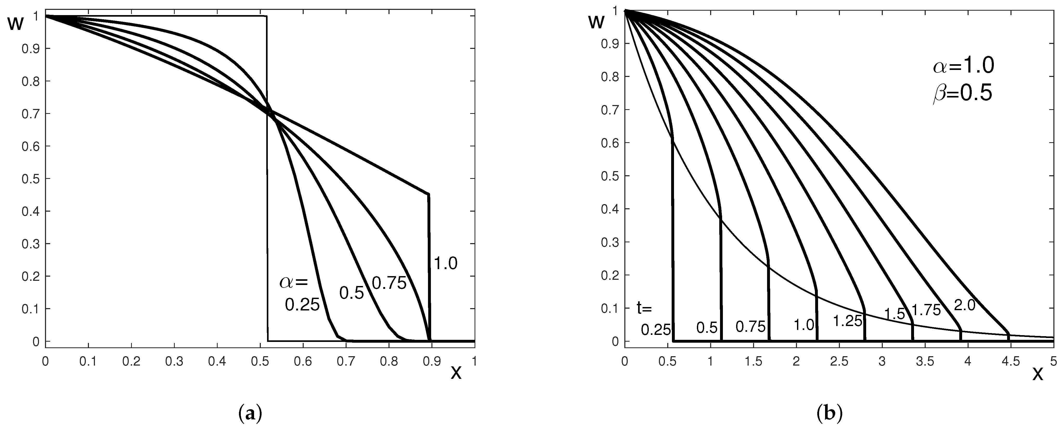
In Figure 1a, the propagation function $w(x,t)$ is plotted for the kernel (64) with $\lambda =0$, which corresponds to the fractional Zener model (1) when $\alpha \in (0,1)$. The function $w(x,t)$ is plotted as a function of x for $t=0.4$ and for different values of the parameter $\alpha$. The limiting case $\alpha =1$ corresponds to the classical integer-order Zener model, where a jump discontinuity is observed at the wave front. The step function given with thinner line corresponds to $\alpha \to 0$, recovering the classical elastic wave equation. For $\alpha \in (0,1)$, we observe, as expected, the coexistence of a finite wave speed and smooth wave front.

In Figure 1b, the propagation function $w(x,t)$ is plotted for the composite kernel (64) with $\alpha =1$, $\lambda =1$ and $\beta =0.5.$ The function $w(x,t)$ is plotted as a function of x for different times t. Since $\alpha =1$, it holds $\kappa >0$, see (40). Therefore, a jump discontinuity at the wave front is expected and observed. The thinner line is the graph of the function $exp(-\kappa x)$ and it marks the height of the jump.

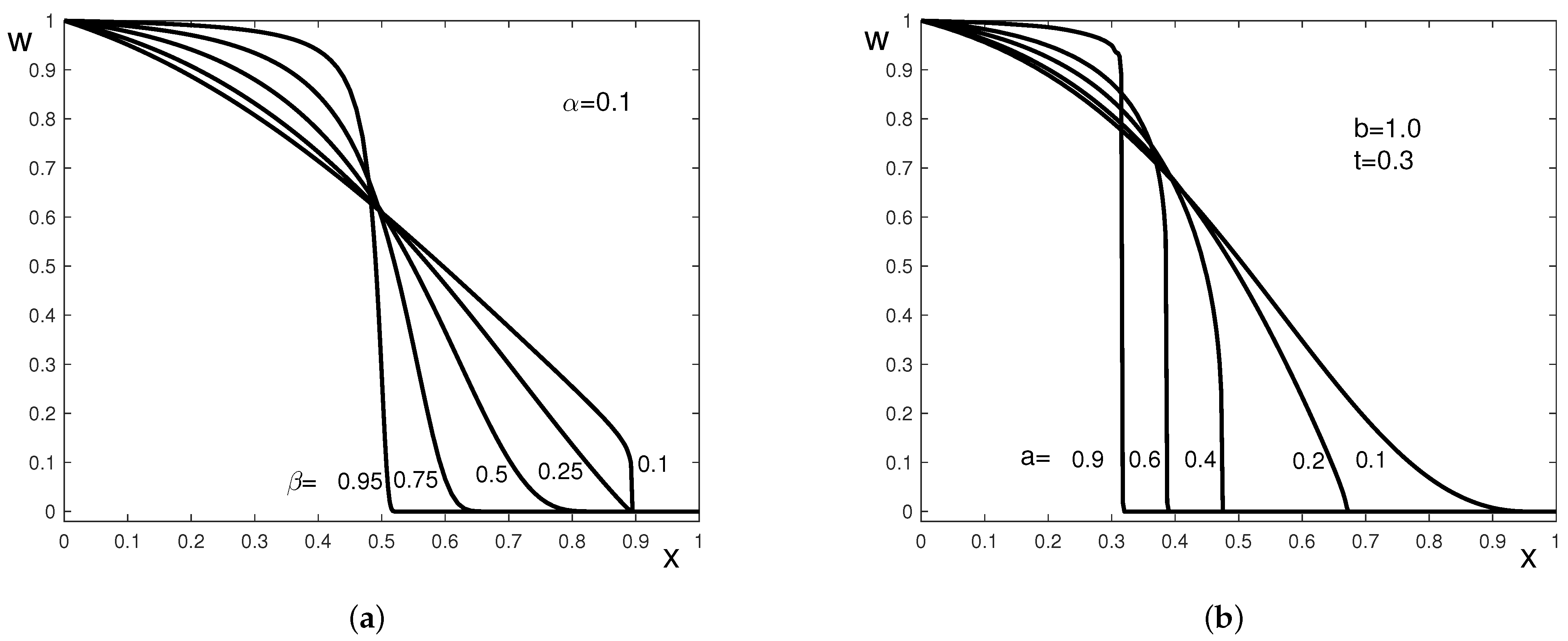
Figure 2a corresponds to the Mittag–Leffler-type kernel (65) with $\alpha =0.1$ and different values of $\beta$, $t=0.4$. Figure 2b corresponds to the distributed-order kernel (66), a takes different values in the interval $(0,1)$, $b=1$, $t=0.3$. In Figure 2, the propagation function $w(x,t)$ is plotted as a function of x. Since ${lim}_{s\to \infty }\widehat{k}\left(s\right)=0$ for the considered kernels, the propagation function is smooth at the wave front.

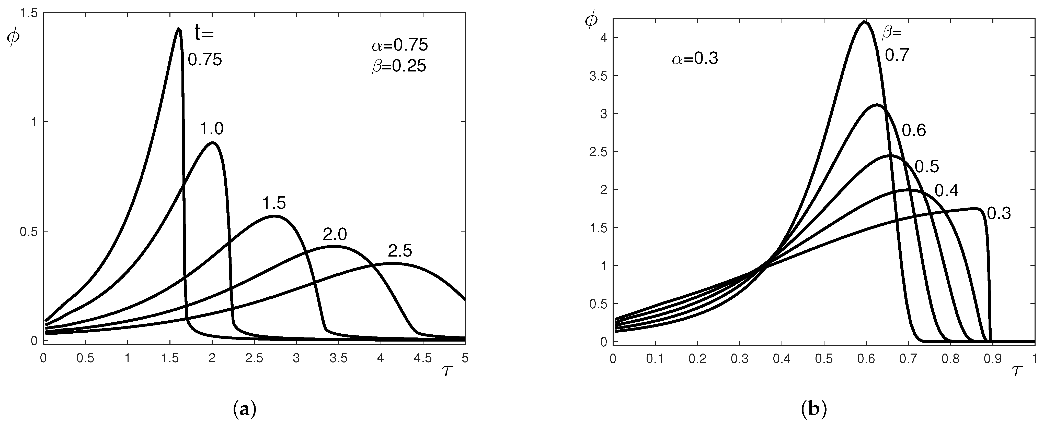
In Figure 3, the subordination function $\varphi$ is plotted as a function of $\tau$ for two types of kernels. Figure 3a corresponds to kernel (64) with $\alpha =0.75$ and $\beta =0.25$, $\lambda =1$. Different values of t are considered. Figure 3b corresponds to the Mittag–Leffler-type kernel (65) with $\alpha =0.3$ and different $\beta$, $\alpha \le \beta <1$; $t=0.4$. The plotted functions in Figure 3 are probability densities as functions of $\tau$.

7. Concluding Remarks

In this work, we study the Zener-type model of a viscoelastic body in the context of general fractional calculus, proposed recently in [26]. The model is studied for a general class of kernels by applying the Bernstein functions technique. This technique allows us to prove that the thermodynamic constraint $a<b$, used in [26], implies not only the dissipation inequality, but also guarantees the complete monotonicity property of the relaxation modulus $G\left(t\right)$, which is a stronger result. Based on this property, the propagation function, which is characteristic for the wave propagation in a viscoelastic medium, is studied and the subordination principle is established for wave equations with generalized Zener-type constitutive law. The subordination identity provides an integral decomposition of the solution into two parts. The first part is a probability density, related to the propagation function and depending only on the constitutive model. The second part is the solution of a related classical wave equation and it depends only on the problem geometry. The analytical findings are supported by numerical work.