Article

Implementation of Analytical Techniques for the Solution of Nonlinear Fractional Order Sawada–Kotera–Ito Equation

1
Department of Mathematics, Abdul Wali Khan University, Mardan 23200, Pakistan
2
Department of Mathematical Sciences College of Sciences, Princess Nourah bint Abdulrahman University, Riyadh 11546, Saudi Arabia
3
Center of Research, Faculty of Engineering, Future University in Egypt, New Cairo 11835, Egypt
4
Fauculty of Computers and Artificial Intelligence, Cairo University, Giza 12613, Egypt
*
Author to whom correspondence should be addressed.
Fractal Fract. 2023, 7(4), 299; https://doi.org/10.3390/fractalfract7040299
Submission received: 20 January 2023 / Revised: 21 February 2023 / Accepted: 15 March 2023 / Published: 29 March 2023

Abstract

:
This article uses the Yang transform decomposition method and the homotopy perturbation transform method to study the seventh-order time-fractional Sawada–Kotera–Ito equation. The fractional derivative is taken into account in the Caputo sense. We used the Yang transform with the Adomian decomposition process and homotopy perturbation procedure on the time-fractional Sawada–Kotera–Ito problem to obtain the solution. We looked at a single case and contrasted it with the actual result to validate the methodologies. These techniques create recurrence relations representing the proposed problem’s solution. We then produced graphical representations that allowed us to visually check all of the outcomes in the proposed case for various fractional order values. The results of applying the current methodologies revealed strong connections to the precise resolution of the problem under investigation. The present study also illustrates error analysis. The numerical results obtained using the suggested techniques show that the methods are both simple and have excellent computational merit.

1. Introduction

The general extension of the integer-order calculus to arbitrary order is known as fractional calculus, which includes integration and differentiation with noninteger order. The origins of fractional calculus can be found in a letter from l’Hopital to Leibniz in 1695, in which he speculated on the meaning of the symbol  d 1 2 x ( t ) d t 1 2 , which denotes the semiderivative of  x ( t )  with respect to  t . Fractional calculus has recently developed into a potent tool as a result of its advantageous characteristics. The foundation for fractional calculus [1,2,3,4] was laid by numerous innovative investigations that provided various definitions of fractional calculus. With the swift growth in digital computer knowledge, many researchers began to work on the theory and applications of fractional calculus. The theory of fractional-order calculus has been used for practical applications, being applied to signal processing [5], chaos theory [6], optics [7], noisy environments [8], and other areas.
Researchers have been drawn to fractional differential equations because they can be used to model a wide range of phenomena, including those relating to epidemic diseases, biomedical applications, viscoelasticity, biology, hydrology, electricity, chemical physics, electrochemistry, probability theory, dynamical systems, heat conduction, and others [9,10,11,12,13]. Classical integer-order differential equations are not capable of capturing the property of memory. As a result, derivatives having an order fraction can be utilised to model memory and inherited traits across a range of domains in terms of fractional-order differential equations. Sun et al. [14] presented a number of real-world applications for fractional calculus in engineering and science. Nonlinear equations are crucial for describing a wide variety of events, with applications in solid state physics, electromagnetic radiation, optical fibers, plasma physics, fluid dynamics, as well as in the disciplines of biology and chemistry. Very few problems in physics, or in fact in any discipline of natural science, can be solved directly. Numerous techniques have been developed to examine the precise and computational solutions of fractional differential equations as a result of their significance in many different domains. The divergence and convergence of the solutions, in addition to the modelling, are equally significant.
Finding analytical solutions to fractional differential equations can be exceedingly challenging in some instances. The importance of creating numerical solutions to these problems has increased as a result. The literature contains many successful strategies for developing semi-analytical and computational methods for fractional differential equations, including the extended direct algebraic method [15], the first integral method [16], the finite difference method [17], the modified Kudryashov method [18], the Adomian decomposition method [19], the optimal homotopy asymptotic method (OHAM) [20], the homotopy perturbation transform technique [21], the standard reductive perturbation method [22], the Haar wavelet method [23], the Elzaki transform decomposition method [24], the differential transform method [25], the fractional sub-equation method [26], and the variational iteration procedure with transformation [27].
A nonlinear PDE called the Kortweg–de Vries (KdV) equation is used to simulate travelling waves in shallow water and harmonic crystal. Boussinesq proposed the KdV hypothesis in 1877 and Kortweg–de Vries provided a conclusion around 1895. In addition, Pomeau et al. [28] introduced the well-known KdV equation of order seven in a study to investigate its stability in the presence of a unique (restricted) perturbation. The seventh-order time-fractional Sawada–Kotera–Ito form of the equation has been addressed as follows:
D t λ F ( x , t ) = 252 F 3 ( x , t ) F x ( x , t ) 63 F x 3 ( x , t ) 378 F ( x , t ) F x ( x , t ) F x x ( x , t ) 126 F 2 ( x , t ) F x x x ( x , t ) 63 F x x ( x , t ) F x x x ( x , t ) 42 F x ( x , t ) F x x x x ( x , t ) 21 F ( x , t ) F x x x x x ( x , t ) F x x x x x x x ( x , t ) , 0 < λ 1 ,
subjected to initial source
F ( x , 0 ) = 4 3 ρ 2 ( 2 3 tanh 2 ( ρ x ) ) .
Recently, various approaches have been used to treat the seventh-order time-fractional Sawada–Kotera–Ito equations, namely, the homotopy analysis scheme [29], the Adomian decomposition method [30], the fractional reduced differential transform technique [31], the q-homotopy analysis approach [32], Lie symmetry analysis [33], the  ( G G ) -expansion method [34], the exp-function method [35], and so forth. The major goal of this paper is to apply the Yang transform decomposition method and the homotopy perturbation transform method to the seventh-order time-fractional Sawada–Kotera–Ito equation (TFSKIE) in the context of the Caputo derivative. The Yang transform and the decomposition method are combined to generate YTDM. Xiao-Jun Yang presented the Yang transform, which can be utilized to solve various differential equations having constant coefficients [36]. In contrast to the standard Adomian process, the proposed method does not involve the computation of the fractional derivative or fractional integrals in the recursive mechanism, which makes it easier to estimate the series terms. Round-off errors are avoided by YTDM since they do not require prescribed assumptions, linearization, discretization, or perturbation. YTDM is used in the literature to solve a variety of differential equations, such as, the fractional Belousov–Zhabotinskii reaction [37], the time-fractional Fisher’s equation [38] and many more. The HPTM combines He’s polynomials, the Yang transform, and the homotopy perturbation method. He’s polynomials can be used to handle the nonlinear terms with simplicity. The proposed method’s analytical results demonstrate how easily implemented and highly desirable the method is computationally.
The present work is arranged as follows: In Section 2, we begin with the basic concept of the fractional calculus. In Section 3 and Section 4, we present the basic idea of the proposed methods. In Section 5, we apply these methods to solve the Sawada–Kotera–Ito equation with the given initial conditions. Finally, the conclusions are provided in Section 6.

2. Basic Concept

In this framework, FC and the Yang transform (YT) will be used. We provide a reminder of their definitions and notations.
Definition 1.
The Caputo operator fractional derivative is defined by [39]
D t λ F ( x , t ) = 1 Γ ( k λ ) 0 t ( t λ ) k λ 1 F ( k ) ( x , λ ) d λ , k 1 < λ k , k N .
Definition 2.
The YT of the function is represented by
Y { F ( t ) } = M ( u ) = 0 e t u F ( t ) d t , t > 0 ,
here u is the transform variable.
Some important functions with YT are stated as.
Y [ 1 ] = u , Y [ t ] = u 2 , Y [ t q ] = Γ ( q + 1 ) u q + 1 .
and inverse YT is
Y 1 { M ( u ) } = F ( t ) .
Definition 3.
The YT of the nth derivative function is represented by
Y { F n ( t ) } = M ( u ) u n k = 0 n 1 F k ( 0 ) u n k 1 , n = 1 , 2 , 3 ,
Definition 4.
The YT of the fractional derivative function is represented by
Y { F λ ( t ) } = M ( u ) u λ k = 0 n 1 F k ( 0 ) u λ ( k + 1 ) , 0 < λ n .

3. Fundamental Concept of HPTM

Here, the general methodology of HPTM is given to solve FPDE.
D t λ F ( x , t ) = P 1 [ x ] F ( x , t ) + Q 1 [ x ] F ( x , t ) , 1 < λ 2 ,
subjected to initial sources
F ( x , 0 ) = ξ ( x ) , t F ( x , 0 ) = ξ ( x ) .
Here,  D t λ = λ t λ  is the Caputo type operator,  P 1 [ x ]  is linear and  Q 1 [ x ]  is a nonlinear function.
By utilizing YT, we get
Y [ D t λ F ( x , t ) ] = Y [ P 1 [ x ] F ( x , t ) + Q 1 [ x ] F ( x , t ) ] ,
1 u λ { M ( u ) u F ( 0 ) u 2 F ( 0 ) } = Y [ P 1 [ x ] F ( x , t ) + Q 1 [ x ] F ( x , t ) ] .
On simplifying the above Equation, we get
M ( F ) = u F ( 0 ) + u 2 F ( 0 ) + u λ Y [ P 1 [ x ] F ( x , t ) + Q 1 [ x ] F ( x , t ) ] .
On utilizing the inverse YT, we get
F ( x , t ) = F ( 0 ) + F ( 0 ) + Y 1 [ u λ Y [ P 1 [ x ] F ( x , t ) + Q 1 [ x ] F ( x , t ) ] ] .
According to the standard homotopy perturbation method, the solution  F ( x , t )  can be expanded into infinite series as [40]
F ( x , t ) = k = 0 ϵ k F k ( x , t ) .
with parameter  ϵ [ 0 , 1 ] .
The nonlinear term is considered as
Q 1 [ x ] F ( x , t ) = k = 0 ϵ k H n ( F ) .
In addition,  H k ( F )  represents He’s polynomials [41] and is as
H n ( F 0 , F 1 , . . . , F n ) = 1 Γ ( n + 1 ) D ϵ k Q 1 k = 0 ϵ i F i | ϵ = 0 .
where  D ϵ k = k ϵ k .
By putting (14) and (15) in (12), we have
k = 0 ϵ k F k ( x , t ) = F ( 0 ) + F ( 0 ) + ϵ × Y 1 u λ Y { P 1 k = 0 ϵ k F k ( x , t ) + k = 0 ϵ k H k ( F ) } .
By comparing the coefficient of  ϵ , we obtain
ϵ 0 : F 0 ( x , t ) = F ( 0 ) + F ( 0 ) , ϵ 1 : F 1 ( x , t ) = Y 1 u λ Y ( P 1 [ x ] F 0 ( x , t ) + H 0 ( F ) ) , ϵ 2 : F 2 ( x , t ) = Y 1 u λ Y ( P 1 [ x ] F 1 ( x , t ) + H 1 ( F ) ) , . . . ϵ k : F k ( x , t ) = Y 1 u λ Y ( P 1 [ x ] F k 1 ( x , t ) + H k 1 ( F ) ) , k > 0 , k N .
Lastly, the solution of  F k ( x , t )  is stated as
F ( x , t ) = lim ϵ 1 k = 0 ϵ k F k ( x , t ) .

4. Fundamental Concept of YTDM

Here, the general methodology of YTDM is given to solve FPDE.
D t λ F ( x , t ) = P 1 ( x , t ) + Q 1 ( x , t ) , 0 < λ 1 ,
subjected to initial sources
F ( x , 0 ) = ξ ( x ) , t F ( x , 0 ) = ξ ( x ) .
Here,  D t λ = λ t λ  is the Caputo type operator,  P 1  is a linear and  Q 1  is a non-linear function.
By utilizing YT, we get
Y [ D t λ F ( x , t ) ] = Y [ P 1 ( x , t ) + Q 1 ( x , t ) ] , 1 u λ { M ( u ) u F ( 0 ) u 2 F ( 0 ) } = Y [ P 1 ( x , t ) + Q 1 ( x , t ) ] .
On simplifying the above Equation, we get
M ( F ) = u F ( 0 ) + u 2 F ( 0 ) + u λ Y [ P 1 ( x , t ) + Q 1 ( x , t ) ] ,
On utilizing the inverse YT, we get
F ( x , t ) = F ( 0 ) + F ( 0 ) + Y 1 [ u λ Y [ P 1 ( x , t ) + Q 1 ( x , t ) ] .
The Adomian decomposition method defines the unknown function  F ( x , t )  by an infinite series [42]. Thus, by YTDM
F ( x , t ) = m = 0 F m ( x , t ) .
The nonlinear term is considered as
Q 1 ( x , t ) = m = 0 A m .
with
A m = 1 m ! m m Q 1 k = 0 k x k , k = 0 k t k = 0 ,
By putting (24) and (26) into (23), we get
m = 0 F m ( x , t ) = F ( 0 ) + F ( 0 ) + Y 1 u λ Y P 1 ( m = 0 x m , m = 0 t m ) + m = 0 A m .
Thus, we can write
F 0 ( x , t ) = F ( 0 ) + t F ( 0 ) ,
F 1 ( x , t ) = Y 1 u λ Y + { P 1 ( x 0 , t 0 ) + A 0 } ,
Hence, in general for  m 1 , we have
F m + 1 ( x , t ) = Y 1 u λ Y + { P 1 ( x m , t m ) + A m } .

5. Application

5.1. Example

Let us apply the seventh order Sawada–Kotera–Ito equation, which has the following form:
D t λ F ( x , t ) = 252 F 3 ( x , t ) F x ( x , t ) 63 F x 3 ( x , t ) 378 F ( x , t ) F x ( x , t ) F x x ( x , t ) 126 F 2 ( x , t ) F x x x ( x , t ) 63 F x x ( x , t ) F x x x ( x , t ) 42 F x ( x , t ) F x x x x ( x , t ) 21 F ( x , t ) F x x x x x ( x , t ) F x x x x x x x ( x , t ) , 0 < λ 1 ,
subjected to initial source
F ( x , 0 ) = 4 3 ρ 2 ( 2 3 tanh 2 ( ρ x ) ) .
  • Case I: Implementation of HPTM
By utilizing YT, we get
Y λ F t λ = Y [ 252 F 3 ( x , t ) F x ( x , t ) 63 F x 3 ( x , t ) 378 F ( x , t ) F x ( x , t ) F x x ( x , t ) 126 F 2 ( x , t ) F x x x ( x , t ) 63 F x x ( x , t ) F x x x ( x , t ) 42 F x ( x , t ) F x x x x ( x , t ) 21 F ( x , t ) F x x x x x ( x , t ) F x x x x x x x ( x , t ) ] ,
On simplifying the above Equation, we get
1 u λ { M ( u ) u F ( 0 ) } = Y [ 252 F 3 ( x , t ) F x ( x , t ) 63 F x 3 ( x , t ) 378 F ( x , t ) F x ( x , t ) F x x ( x , t ) 126 F 2 ( x , t ) F x x x ( x , t ) 63 F x x ( x , t ) F x x x ( x , t ) 42 F x ( x , t ) F x x x x ( x , t ) 21 F ( x , t ) F x x x x x ( x , t ) F x x x x x x x ( x , t ) ] ,
M ( u ) = u F ( 0 ) + u λ [ 252 F 3 ( x , t ) F x ( x , t ) 63 F x 3 ( x , t ) 378 F ( x , t ) F x ( x , t ) F x x ( x , t ) 126 F 2 ( x , t ) F x x x ( x , t ) 63 F x x ( x , t ) F x x x ( x , t ) 42 F x ( x , t ) F x x x x ( x , t ) 21 F ( x , t ) F x x x x x ( x , t ) F x x x x x x x ( x , t ) ] .
On utilizing the inverse YT, we get
F ( x , t ) = F ( 0 ) + Y 1 [ u λ { Y ( 252 F 3 ( x , t ) F x ( x , t ) 63 F x 3 ( x , t ) 378 F ( x , t ) F x ( x , t ) F x x ( x , t ) 126 F 2 ( x , t ) F x x x ( x , t ) 63 F x x ( x , t ) F x x x ( x , t ) 42 F x ( x , t ) F x x x x ( x , t ) 21 F ( x , t ) F x x x x x ( x , t ) F x x x x x x x ( x , t ) ) } ] , F ( x , t ) = 4 3 ρ 2 ( 2 3 tanh 2 ( ρ x ) ) + Y 1 [ u λ { Y ( 252 F 3 ( x , t ) F x ( x , t ) 63 F x 3 ( x , t ) 378 F ( x , t ) F x ( x , t ) F x x ( x , t ) 126 F 2 ( x , t ) F x x x ( x , t ) 63 F x x ( x , t ) F x x x ( x , t ) 42 F x ( x , t ) F x x x x ( x , t ) 21 F ( x , t ) F x x x x x ( x , t ) F x x x x x x x ( x , t ) ) } ] .
Thus, by HPM, the non-linear terms are used in the form of He’s polynomial  H k ( F )  as
k = 0 ϵ k F k ( x , t ) = 4 3 ρ 2 ( 2 3 tanh 2 ( ρ x ) ) + ϵ ( Y 1 [ u λ Y [ 252 k = 0 ϵ k H k ( F ) 63 k = 0 ϵ k H k ( F ) 378 k = 0 ϵ k H k ( F ) 126 k = 0 ϵ k H k ( F ) 63 k = 0 ϵ k H k ( F ) 42 k = 0 ϵ k H k ( F ) 21 k = 0 ϵ k H k ( F ) k = 0 ϵ k F k ( x , t ) x x x x x x x ] ] ) .
On comparing the coefficient of  ϵ , we have
ϵ 0 : F 0 ( x , t ) = 4 3 ρ 2 ( 2 3 tanh 2 ( ρ x ) ) , ϵ 1 : F 1 ( x , t ) = 2048 ρ 9 t λ tanh ( ρ x ) sech 2 ( ρ x ) Γ ( λ + 1 ) , ϵ 2 : F 2 ( x , t ) = 524,288 ρ 16 t 2 λ ( cosh ( 2 ρ x ) 2 ) sech 4 ( ρ x ) 9 Γ ( 2 λ + 1 ) ,
The obtained solution can be taken in series form as
F ( x , t ) = F 0 ( x , t ) + F 1 ( x , t ) + F 2 ( x , t ) + F ( x , t ) = 4 3 ρ 2 ( 2 3 tanh 2 ( ρ x ) ) 2048 ρ 9 t λ tanh ( ρ x ) sech 2 ( ρ x ) Γ ( λ + 1 ) + 524,288 ρ 16 t 2 λ ( cosh ( 2 ρ x ) 2 ) sech 4 ( ρ x ) 9 Γ ( 2 λ + 1 ) +
  • Case II: Implementation of YTDM
By utilizing YT, we get
Y λ F t λ = Y [ 252 F 3 ( x , t ) F x ( x , t ) 63 F x 3 ( x , t ) 378 F ( x , t ) F x ( x , t ) F x x ( x , t ) 126 F 2 ( x , t ) F x x x ( x , t ) 63 F x x ( x , t ) F x x x ( x , t ) 42 F x ( x , t ) F x x x x ( x , t ) 21 F ( x , t ) F x x x x x ( x , t ) F x x x x x x x ( x , t ) ] ,
On simplifying the above Equation, we get
1 u λ { M ( u ) u F ( 0 ) } = Y [ 252 F 3 ( x , t ) F x ( x , t ) 63 F x 3 ( x , t ) 378 F ( x , t ) F x ( x , t ) F x x ( x , t ) 126 F 2 ( x , t ) F x x x ( x , t ) 63 F x x ( x , t ) F x x x ( x , t ) 42 F x ( x , t ) F x x x x ( x , t ) 21 F ( x , t ) F x x x x x ( x , t ) F x x x x x x x ( x , t ) ] ,
M ( u ) = u F ( 0 ) + u λ Y [ 252 F 3 ( x , t ) F x ( x , t ) 63 F x 3 ( x , t ) 378 F ( x , t ) F x ( x , t ) F x x ( x , t ) 126 F 2 ( x , t ) F x x x ( x , t ) 63 F x x ( x , t ) F x x x ( x , t ) 42 F x ( x , t ) F x x x x ( x , t ) 21 F ( x , t ) F x x x x x ( x , t ) F x x x x x x x ( x , t ) ] .
On utilizing the inverse YT, we get
F ( x , t ) = F ( 0 ) + Y 1 [ u λ { Y [ 252 F 3 ( x , t ) F x ( x , t ) 63 F x 3 ( x , t ) 378 F ( x , t ) F x ( x , t ) F x x ( x , t ) 126 F 2 ( x , t ) F x x x ( x , t ) 63 F x x ( x , t ) F x x x ( x , t ) 42 F x ( x , t ) F x x x x ( x , t ) 21 F ( x , t ) F x x x x x ( x , t ) F x x x x x x x ( x , t ) ] } ] , F ( x , t ) = 4 3 ρ 2 ( 2 3 tanh 2 ( ρ x ) ) + Y 1 [ u λ { Y [ 252 F 3 ( x , t ) F x ( x , t ) 63 F x 3 ( x , t ) 378 F ( x , t ) F x ( x , t ) F x x ( x , t ) 126 F 2 ( x , t ) F x x x ( x , t ) 63 F x x ( x , t ) F x x x ( x , t ) 42 F x ( x , t ) F x x x x ( x , t ) 21 F ( x , t ) F x x x x x ( x , t ) F x x x x x x x ( x , t ) ] } ] .
Thus, the solution in series form is taken as
F ( x , t ) = m = 0 F m ( x , t ) .
Let us solve the nonlinear terms using the Adomian polynomial as  F 3 ( x , t ) F x ( x , t ) = m = 0 A m , F x 3 ( x , t ) = m = 0 B m , F ( x , t ) F x ( x , t ) F x x ( x , t ) = m = 0 C m , F 2 ( x , t ) F x x x ( x , t ) = m = 0 D m , F x x ( x , t ) F x x x ( x , t ) = m = 0 E m , F x ( x , t ) F x x x x ( x , t ) = m = 0 F m , F ( x , t ) F x x x x x ( x , t ) = m = 0 G m .  Hence, we have
m = 0 F m ( x , t ) = F ( x , 0 ) + Y 1 [ u λ Y [ 252 m = 0 A m 63 m = 0 B m 378 m = 0 C m 126 m = 0 D m 63 m = 0 E m 42 m = 0 F m 21 m = 0 G m F x x x x x x x ( x , t ) ] ] , m = 0 F m ( x , t ) = 4 3 ρ 2 ( 2 3 tanh 2 ( ρ x ) ) + Y 1 [ u λ Y [ 252 m = 0 A m 63 m = 0 B m 378 m = 0 C m 126 m = 0 D m 63 m = 0 E m 42 m = 0 F m 21 m = 0 G m F x x x x x x x ( x , t ) ] ] .
On comparing both sides, we have
F 0 ( x , t ) = 4 3 ρ 2 ( 2 3 tanh 2 ( ρ x ) ) ,
On  m = 0
F 1 ( x , t ) = 2048 ρ 9 t λ tanh ( ρ x ) sech 2 ( ρ x ) Γ ( λ + 1 ) ,
On  m = 1
F 2 ( x , t ) = 524,288 ρ 16 t 2 λ ( cosh ( 2 ρ x ) 2 ) sech 4 ( ρ x ) 9 Γ ( 2 λ + 1 ) ,
So, in the same sense, the other terms for  ( m 3 )  are easy to obtain
F ( x , t ) = m = 0 F m ( x , t ) = F 0 ( x , t ) + F 1 ( x , t ) + F 2 ( x , t ) +
F ( x , t ) = 4 3 ρ 2 ( 2 3 tanh 2 ( ρ x ) ) 2048 ρ 9 t λ tanh ( ρ x ) sech 2 ( ρ x ) Γ ( λ + 1 ) + 524,288 ρ 16 t 2 λ ( cosh ( 2 ρ x ) 2 ) sech 4 ( ρ x ) 9 Γ ( 2 λ + 1 ) +
By taking  λ = 1 , we get
F ( x , t ) = 4 3 ρ 2 ( 2 3 tanh 2 ( ρ ( 256 ρ 6 t 3 + x ) ) )

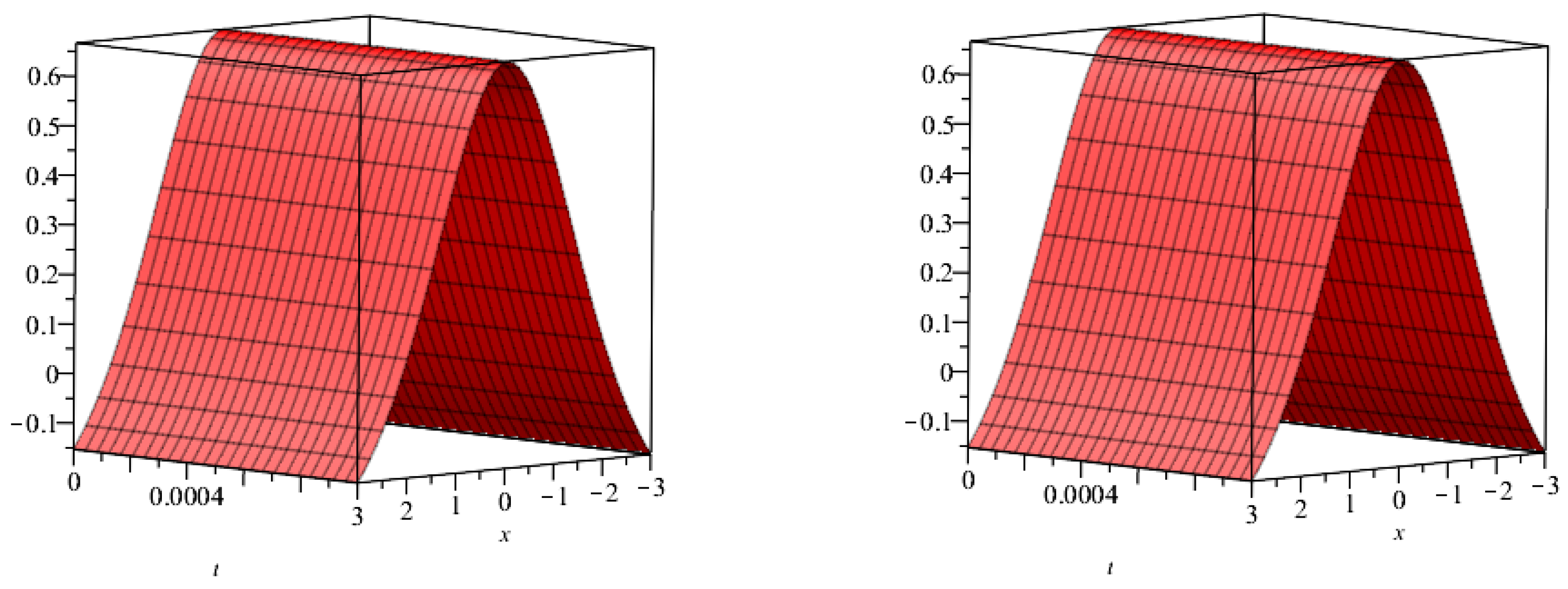
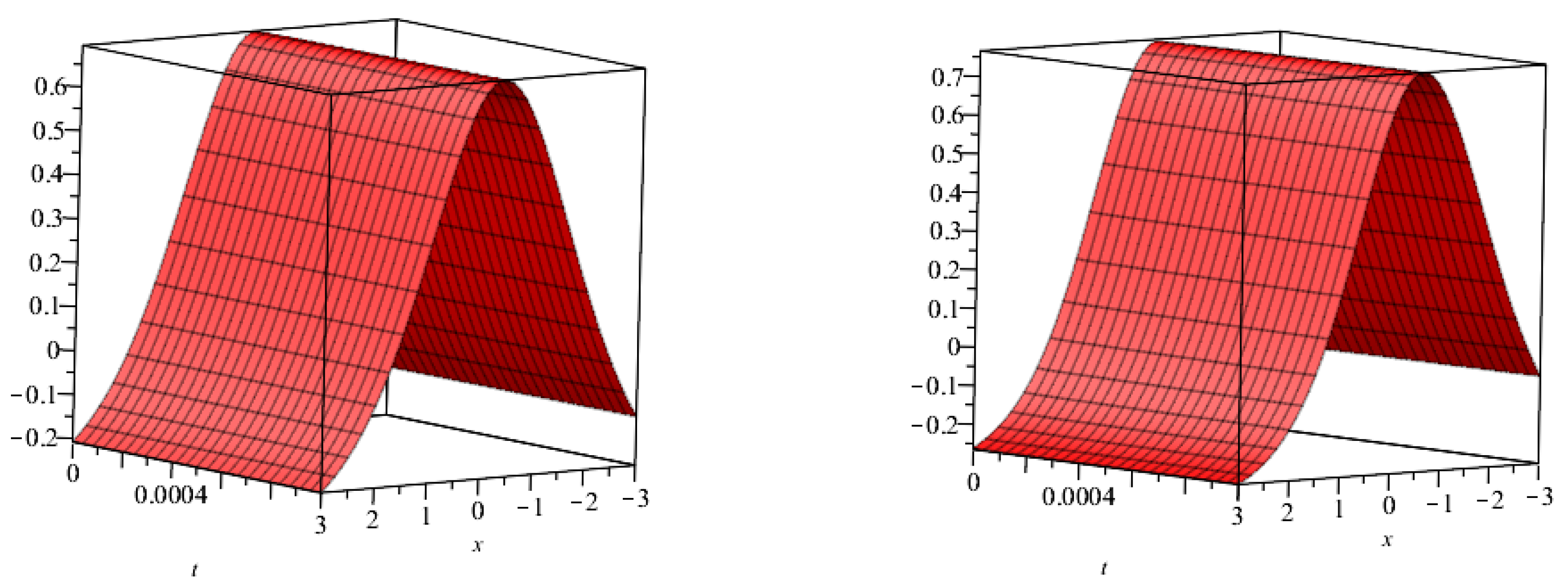
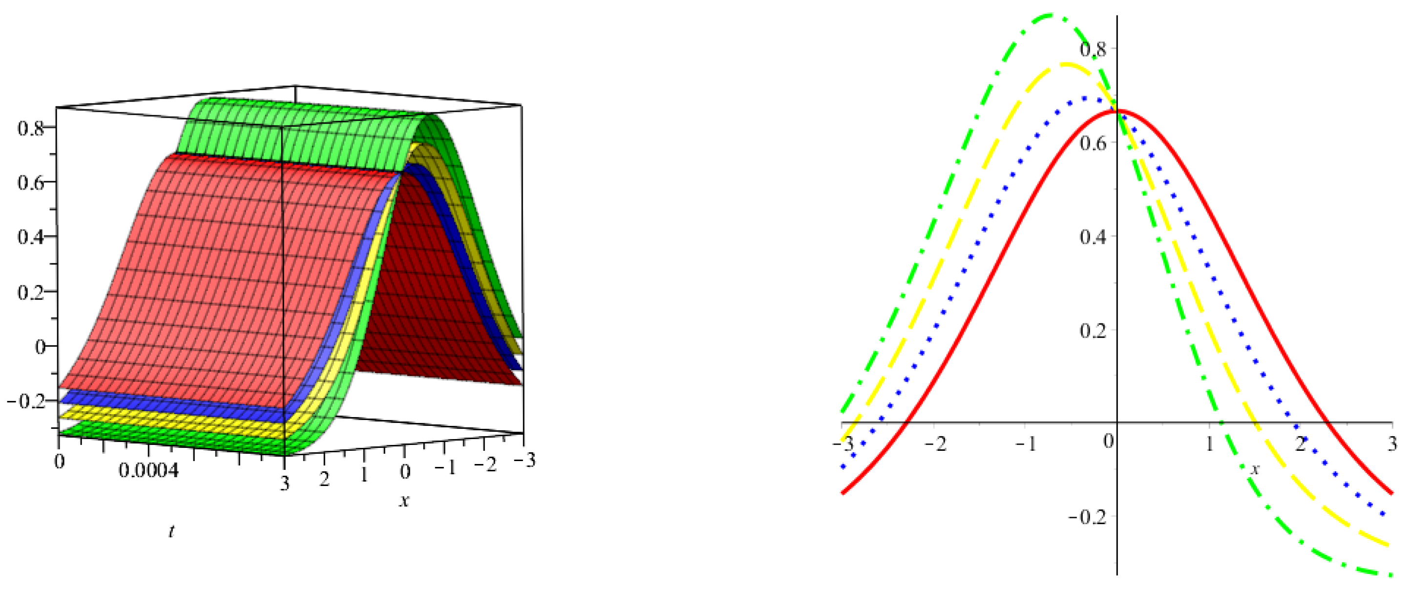
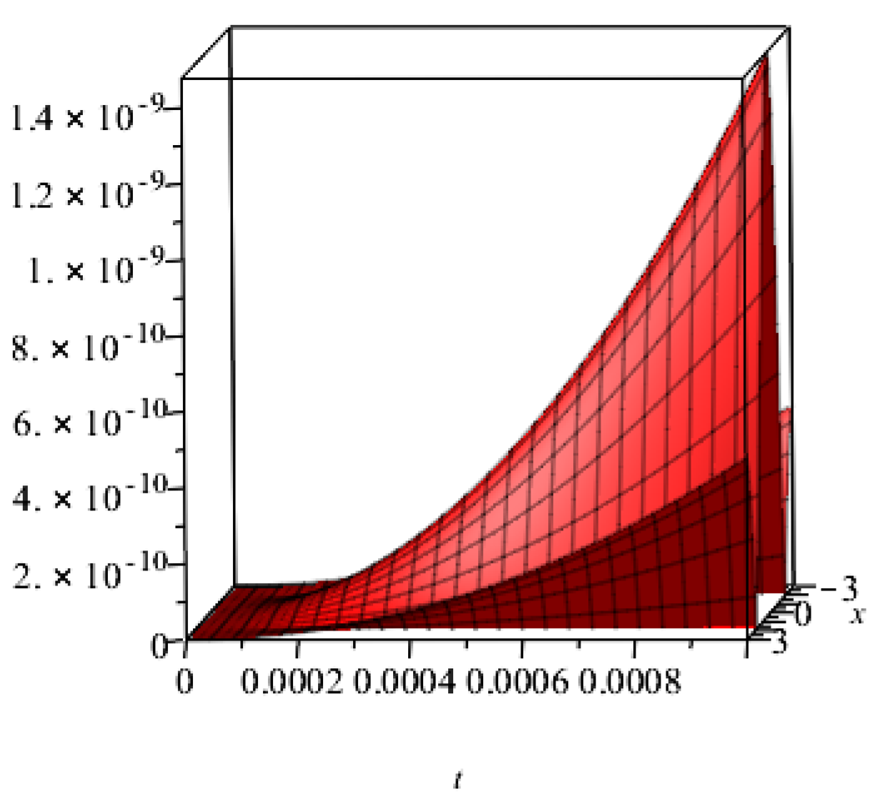
5.2. Numerical Simulation Studies

An approximate analytical solution to the  F ( x , t )  is provided in this section. The method’s applicability is demonstrated by the numerical results, and its correctness is assessed in comparison to exact results. Application of our method produces a good performance and simple results that can be easily implemented. The exact solution plot, which is shown in Figure 1, was compared to the solution plot of  F ( x , t ) . Figure 2 displays the graphical representations of  F ( x , t )  for  λ = 0.8  and  0.6 . Similarly, Figure 3 displays the plots of  F ( x , t )  for various values of  λ = 0.25 , 0.50 , 0.75 , 1 , while Figure 4 displays the behaviour of the absolute error for the same equation derived using both methodologies. The approximate solution to the equation  F ( x , t )  is shown in Table 1 for various values of  x  and  t , while the absolute error comparison is shown in Table 2 for various values of  x  and  t . It should be mentioned that we obtained a good approximation with the exact solution of the stated problems and that we employed third-order approximate solutions throughout the computations. If we increased the order of the approximation, which would increase the number of terms in the solution, better approximation solutions would be found.

6. Conclusions

In the current work, we successfully applied two unique techniques termed YTDM and HPTM to find the solution for TFSKIE in a Caputo derivative manner. The Yang transform was combined with He’s polynomials and the homotopy perturbation method in the first technique, while the Adomian polynomials and the decomposition method were combined in the second method. The solution graphs display the different helpful dynamics of the problem at various fractional orders of the derivatives. The concept that fractional solutions converge to the integer-order solution was tested using numerical results and graphs. The investigation has demonstrated the best connection of the suggested methods with the precise solutions of the problem. These novel methods give results that are more accurate numerically and require less time and computational effort. The research described leads to the conclusion that the suggested techniques can be simply adapted to handle other scientific and engineering problems.

Author Contributions

Methodology, R.S. and F.M.; Software, E.M.T. and N.A.G.; Investigation, F.M.; Writing—original draft, R.S and E.M.T. All authors have read and agreed to the published version of the manuscript.

Funding

The author, Fatemah Mofarreh, expresses her gratitude to Princess Nourah bint Abdulrahman University Researchers Supporting Project number (PNURSP2023R27), Princess Nourah bint Abdulrahman University, Riyadh, Saudi Arabia.

Data Availability Statement

The numerical data used to support the findings of this study are included within the article.

Acknowledgments

The author, Fatemah Mofarreh, expresses her gratitude to Princess Nourah bint Abdulrahman University Researchers Supporting Project number (PNURSP2023R27), Princess Nourah bint Abdulrahman University, Riyadh, Saudi Arabia.

Conflicts of Interest

The authors declare no conflict of interest.

References

  1. Riemann, G.F.B. Versuch einer allgemeinen Auffassung der integration und differentiation. In Gesammelte Mathematische Werke; Druck: Leipzig, Germany, 1896. [Google Scholar]
  2. Caputo, M. Elasticità e Dissipazione; Zanichelli: Bologna, Italy, 1969. [Google Scholar]
  3. Miller, K.S.; Ross, B. An Introduction to Fractional Calculus and Fractional Differential Equations; Wiley: New York, NY, USA, 1993. [Google Scholar]
  4. Podlubny, I. Fractional Differential Equations; Academic Press: New York, NY, USA, 1999. [Google Scholar]
  5. Li, Y.; Liu, F.; Turner, I.W.; Li, T. Time-fractional diffusion equation for signal smoothing. Appl Math Comput. 2018, 326, 108–116. [Google Scholar] [CrossRef] [Green Version]
  6. Lin, W. Global existence theory and chaos control of fractional differential equations. J. Math. Anal. Appl. 2007, 332, 709–726. [Google Scholar] [CrossRef] [Green Version]
  7. Bulut, H.; Sulaiman, T.A.; Baskonus, H.M.; Rezazadeh, H.; Eslami, M.; Mirzazadeh, M. Optical solitons and other solutions to the conformable space-time fractional Fokas-Lenells equation. Optik 2018, 172, 20–27. [Google Scholar] [CrossRef]
  8. Liu, D.Y.; Gibaru, O.; Perruquetti, W.; Laleg-Kirati, T.M. Fractional order differentiation by integration and error analysis in noisy environment. IEEE Trans. Autom. Control. 2015, 60, 2945–2960. [Google Scholar] [CrossRef]
  9. Hilfer, R. Applications of Fractional Calculus in Physics; World Scientific Publishing Co., Inc.: River Edge, NJ, USA, 2000. [Google Scholar]
  10. Laroche, E.; Knittel, D. An improved linear fractional model for robustness analysis of a winding system. Control. Eng. Pract. 2005, 13, 659–666. [Google Scholar] [CrossRef]
  11. Monje, C.; Vinagre, B.; Feliu, V.; Chen, Y. Tuning and auto tuning of fractional order controllers for industry applications. Control. Eng. Pract. 2008, 16, 798–812. [Google Scholar] [CrossRef] [Green Version]
  12. Sabatier, J.; Aoun, M.; Oustaloup, A.; Grgoire, G.; Ragot, F.; Roy, P. Fractional system identification for lead acid battery state of charge estimation. Signal Process. 2006, 86, 2645–2657. [Google Scholar] [CrossRef]
  13. Vinagre, B.; Monje, C.; Calderon, A.; Suarej, J. Fractional PID controllers for industry application: A brief introduction. J. Vib. Control. 2007, 13, 1419–1430. [Google Scholar] [CrossRef]
  14. Sun, H.G.; Zhang, Y.; Baleanu, D.; Chen, W.; Chen, Y.Q. A new collection of real world applications of fractional calculus in science and engineering. Commun. Nonlinear Sci. Numer. Simul. 2018, 64, 213–231. [Google Scholar] [CrossRef]
  15. Younis, M.; Iftikhar, M. Computational examples of a class of fractional order nonlinear evolution equations using modified extended direct algebraic method. J. Comput. Methods 2015, 15, 359–365. [Google Scholar] [CrossRef]
  16. Eslami, M.; Fathi Vajargah, B.; Mirzazadeh, M.; Biswas, A. Application of first integral method to fractional partial differential equations. Indian J. Phys. 2014, 88, 177–184. [Google Scholar] [CrossRef]
  17. Meerschaert, M.M.; Tadjeran, C. Finite difference approximations for two-sided space-fractional partial differential equations. Appl. Numer. Math. 2006, 56, 80–90. [Google Scholar] [CrossRef]
  18. Gaber, A.A.; Aljohani, A.F.; Ebaid, A.; Machado, J.T. The generalized Kudryashov method for nonlinear space-time fractional partial differential equations of Burgers type. Nonlinear Dyn. 2019, 95, 361–368. [Google Scholar] [CrossRef]
  19. El-Wakil, S.A.; Elhanbaly, A.; Abdou, M.A. Adomian decomposition method for solving fractional nonlinear differential equations. Appl. Math. Comput. 2006, 182, 13–324. [Google Scholar] [CrossRef]
  20. Sarwar, S.; Alkhalaf, S.; Iqbal, S.; Zahid, M.A. A note on optimal homotopy asymptotic method for the solutions of fractional order heat-and wave-like partial differential equations. Comput. Math. Appl. 2015, 70, 942–953. [Google Scholar] [CrossRef]
  21. Sunthrayuth, P.; Alyousef, H.A.; El-Tantawy, S.A.; Khan, A.; Wyal, N. Solving Fractional-Order Diffusion Equations in a Plasma and Fluids via a Novel Transform. J. Funct. Spaces 2022, 2022, 1899130. [Google Scholar] [CrossRef]
  22. Uddin, M.F.; Hafez, M.G.; Hwang, I.; Park, C. Effect of Space Fractional Parameter on Nonlinear Ion Acoustic Shock Wave Excitation in an Unmagnetized Relativistic Plasma. Front. Phys. 2022, 9, 766. [Google Scholar] [CrossRef]
  23. Wang, L.; Ma, Y.; Meng, Z. Haar wavelet method for solving fractional partial differential equations numerically. Appl. Math. Comput. 2014, 227, 66–76. [Google Scholar] [CrossRef]
  24. Nonlaopon, K.; Alsharif, A.M.; Zidan, A.M.; Khan, A.; Hamed, Y.S.; Shah, R. Numerical investigation of fractional-order Swift-Hohenberg equations via a Novel transform. Symmetry 2021, 13, 1263. [Google Scholar] [CrossRef]
  25. Odibat, Z.; Momani, S. A generalized differential transform method for linear partial differential equations of fractional order. Appl. Math. Lett. 2008, 21, 194–199. [Google Scholar] [CrossRef] [Green Version]
  26. Zheng, B.; Wen, C. Exact solutions for fractional partial differential equations by a new fractional sub-equation method. Adv. Differ. Equ. 2013, 2013, 1–12. [Google Scholar] [CrossRef] [Green Version]
  27. Alyobi, S.; Shah, R.; Khan, A.; Shah, N.A.; Nonlaopon, K. Fractional Analysis of Nonlinear Boussinesq Equation under Atangana-Baleanu-Caputo Operator. Symmetry 2022, 14, 2417. [Google Scholar] [CrossRef]
  28. Pomeau, Y.; Ramani, A.; Grammaticos, B. Structural stability of the Korteweg-de Vries solitons under a singular perturbation. Phys. D 1988, 31, 27–134. [Google Scholar] [CrossRef]
  29. Arora, R.; Sharma, H. Application of HAM to seventh order KdV equations. Int. J. Syst. Assur. Eng. Manag. 2018, 9, 131–138. [Google Scholar] [CrossRef]
  30. El-Sayed, S.M.; Kaya, D. An application of the ADM to seven-order Sawada-Kotara equations. Appl. Math. Comput. 2004, 157, 93–101. [Google Scholar] [CrossRef]
  31. Jena, R.M.; Chakraverty, S.; Jena, S.K.; Sedighi, H.M. On the wave solutions of time-fractional Sawada-Kotera-Ito equation arising in shallow water. Math. Methods Appl Sci. 2021, 44, 583–592. [Google Scholar] [CrossRef]
  32. Akinyemi, L. q-Homotopy analysis method for solving the seventh-order time-fractional Lax’s Korteweg-de Vries and Sawada-Kotera equations. Comput. Appl. Math. 2019, 38, 191. [Google Scholar] [CrossRef]
  33. Yaşar, E.; Yildirim, Y.; Khalique, C.M. Lie symmetry analysis, conservation laws and exact solutions of the seventh-order time fractional Sawada-Kotera-Ito equation. Results Phys. 2016, 6, 322–328. [Google Scholar] [CrossRef] [Green Version]
  34. Al-Shawba, A.A.; Gepreel, K.A.; Abdullah, F.A.; Azmi, A. Abundant closed form solutions of the conformable time fractional Sawada-Kotera-Ito equation using (G’/G)-expansion method. Results Phys. 2018, 9, 337–343. [Google Scholar] [CrossRef]
  35. Guner, O. New exact solutions for the seventh-order time fractional Sawada-Kotera-Ito equation via various methods. Waves Random Complex Media 2020, 30, 441–457. [Google Scholar] [CrossRef]
  36. Yang, X.J.; Baleanu, D.; Srivastava, H.M. Local fractional laplace transform and applications. In Local Fractional Integral Transforms and Their Applications; Academic Press: Cambridge, MA, USA, 2016; p. 147178. [Google Scholar]
  37. Alaoui, M.K.; Fayyaz, R.; Khan, A.; Shah, R.; Abdo, M.S. Analytical investigation of Noyes-Field model for time-fractional Belousov-Zhabotinsky reaction. Complexity 2021, 2021, 3248376. [Google Scholar] [CrossRef]
  38. Zidan, A.M.; Khan, A.; Shah, R.; Alaoui, M.K.; Weera, W. Evaluation of time-fractional Fisher’s equations with the help of analytical methods. Aims Math. 2022, 7, 18746–18766. [Google Scholar] [CrossRef]
  39. Sunthrayuth, P.; Ullah, R.; Khan, A.; Shah, R.; Kafle, J.; Mahariq, I.; Jarad, F. Numerical analysis of the fractional-order nonlinear system of Volterra integro-differential equations. J. Funct. Spaces 2021, 2021, 1537958. [Google Scholar] [CrossRef]
  40. He, J.H. A coupling method of homotopy technique and perturbation technique for nonlinear problems. Int. J.-Non-Linear Mech. 2003, 35, 743. [Google Scholar]
  41. Ghorbani, A. Beyond adomian’s polynomials: He polynomials. Chaos Solitons Fractals 2009, 39, 1486–1492. [Google Scholar] [CrossRef]
  42. Adomian, G. A review of the decomposition method in applied mathematics. J. Math. Anal. Appl. 1988, 135, 501–544. [Google Scholar] [CrossRef] [Green Version]
Figure 1. The proposed techniques’ and accurate solution graphically depicted.
Fractalfract 07 00299 g001
Figure 2. The proposed techniques’ solution graphically depicted at  λ = 0.8 , 0.6 .
Fractalfract 07 00299 g002
Figure 3. Graphical representation of the proposed techniques’ solution for various orders of  λ .
Fractalfract 07 00299 g003
Figure 4. Graphical representation in terms of the error of the proposed techniques’ solution.
Fractalfract 07 00299 g004
Table 1. Behavior of the accurate solution and our techniques’ solution for various orders of  λ .
  t x   λ = 0.4   λ = 0.6   λ = 0.8 λ = 1
(Approx)
λ = 1
(Exact)
0.010.20.3237020.3238920.3240810.3242690.324269
0.40.3160670.3164390.3168090.3171790.317179
0.60.3040510.3045910.3051290.3056660.305666
0.80.2880990.2887880.2894740.2901590.290159
10.2687750.2695880.2703990.2712070.271207
0.020.20.3236950.3238860.3240760.3242650.324265
0.40.3160520.3164270.3168000.3171720.317172
0.60.3040290.3045740.3051160.3056560.305656
0.80.2880720.2887660.2894570.2901450.290145
10.2687420.2695620.2703780.2711910.271191
0.030.20.3236880.3238800.3240710.3242620.324262
0.40.3160380.3164160.3167910.3171640.317164
0.60.3040090.3045580.3051030.3056450.305645
0.80.2880460.2887450.2894400.2901320.290132
10.2687120.2695380.2703580.2711750.271175
0.040.20.3236810.3238740.3240670.3242580.324258
0.40.3160250.3164050.3167820.3171570.317157
0.60.3039900.3045420.3050900.3056340.305634
0.80.2880220.2887250.2894230.2901180.290118
10.2686840.2695140.2703390.2711590.271159
0.050.20.3236740.3238690.3240620.3242540.324254
0.40.3160120.3163940.3167730.3171500.317150
0.60.3039720.3045260.3050770.3056240.305624
0.80.2879990.2887050.2894070.2901040.290104
10.2686560.2694910.2703190.2711430.271143
Table 2. Behavior of our techniques’ solution in terms of absolute error for various orders of  λ .
  t x   λ = 0.4   λ = 0.6   λ = 0.8   λ = 1   ( HPTM )   λ = 1   ( YTDM )
0.010.25.6701120000     ×     10 4 3.7742650000   ×   10 4 1.8847270000   ×   10 4 1.4000000000   ×   10 9 1.4000000000   ×   10 9
0.41.1121106000   ×   10 3 7.4026790000   ×   10 4 3.6966280000   ×   10 4 1.4000000000   ×   10 9 1.4000000000   ×   10 9
0.61.6151616000   ×   10 3 1.0751203000   ×   10 3 5.3687630000   ×   10 4 1.2000000000   ×   10 9 1.2000000000   ×   10 9
0.82.0593399000   ×   10 3 1.3707844000   ×   10 3 6.8452050000   ×   10 4 1.1000000000   ×   10 9 1.1000000000   ×   10 9
12.4322300000   ×   10 3 1.6189960000   ×   10 3 8.0846870000   ×   10 4 1.0000000000   ×   10 9 1.0000000000   ×   10 9
0.020.25.7087240000   ×   10 4 3.7973100000   ×   10 4 1.8950170000   ×   10 4 5.7000000000   ×   10 9 5.7000000000   ×   10 9
0.41.1196883000   ×   10 3 7.4479250000   ×   10 4 3.7168560000   ×   10 4 5.5000000000   ×   10 9 5.5000000000   ×   10 9
0.61.6261692000   ×   10 3 1.0816936000   ×   10 3 5.3981620000   ×   10 4 4.9000000000   ×   10 9 4.9000000000   ×   10 9
0.82.0733762000   ×   10 3 1.3791670000   ×   10 3 6.8827050000   ×   10 4 4.2000000000   ×   10 9 4.200000000   ×   10 9
12.4488091000   ×   10 3 1.6288977000   ×   10 3 8.1289880000   ×   10 4 3.5000000000   ×   10 9 3.5000000000   ×   10 9
0.030.25.7415440000   ×   10 4 3.8172350000   ×   10 4 1.9040430000   ×   10 4 1.3000000000   ×   10 8 1.3000000000   ×   10 8
0.41.1261329000   ×   10 3 7.4870780000   ×   10 4 3.7346340000   ×   10 4 1.2300000000   ×   10 8 1.2300000000   ×   10 8
0.61.6355328000   ×   10 3 1.0873838000   ×   10 3 5.4240200000   ×   10 4 1.1000000000   ×   10 8 1.1000000000   ×   10 8
0.82.0853172000   ×   10 3 1.3864244000   ×   10 3 6.9156990000   ×   10 4 9.6000000000   ×   10 9 9.6000000000   ×   10 9
12.4629143000   ×   10 3 1.6374712000   ×   10 3 8.1679760000   ×   10 4 7.8000000000   ×   10 9 7.8000000000   ×   10 9
0.040.25.7708370000   ×   10 4 3.8352100000   ×   10 4 1.9122570000   ×   10 4 2.3200000000   ×   10 8 2.3200000000   ×   10 8
0.41.1318886000   ×   10 3 7.5224370000   ×   10 4 3.7508470000   ×   10 4 2.1900000000   ×   10 8 2.1900000000   ×   10 8
0.61.6438970000   ×   10 3 1.0925244000   ×   10 3 5.4476190000   ×   10 4 1.9700000000   ×   10 8 1.9700000000   ×   10 8
0.82.0959854000   ×   10 3 1.3929824000   ×   10 3 6.9458240000   ×   10 4 1.7000000000   ×   10 8 1.7000000000   ×   10 8
12.4755170000   ×   10 3 1.6452195000   ×   10 3 8.2035840000   ×   10 4 1.3800000000   ×   10 8 1.3800000000   ×   10 8
0.050.25.7976140000   ×   10 4 3.8517720000   ×   10 4 1.9198680000   ×   10 4 3.6100000000   ×   10 8 3.6100000000   ×   10 8
0.41.1371537000   ×   10 3 7.5550530000   ×   10 4 3.7659070000   ×   10 4 3.4100000000   ×   10 8 3.4100000000   ×   10 8
0.61.6515506000   ×   10 3 1.0972681000   ×   10 3 5.4695580000   ×   10 4 3.0800000000   ×   10 8 3.0800000000   ×   10 8
0.82.1057483000   ×   10 3 1.3990351000   ×   10 3 6.9738420000   ×   10 4 2.6500000000   ×   10 8 2.6500000000   ×   10 8
12.4870511000   ×   10 3 1.6523716000   ×   10 3 8.2367100000   ×   10 4 2.1700000000   ×   10 8 2.1700000000   ×   10 8
Disclaimer/Publisher’s Note: The statements, opinions and data contained in all publications are solely those of the individual author(s) and contributor(s) and not of MDPI and/or the editor(s). MDPI and/or the editor(s) disclaim responsibility for any injury to people or property resulting from any ideas, methods, instructions or products referred to in the content.

