Fixed-Time Sliding Mode Synchronization of Uncertain Fractional-Order Hyperchaotic Systems by Using a Novel Non-Singleton-Interval Type-2 Probabilistic Fuzzy Neural Network

Abstract

In this study, we proposed a sliding mode control method based on fixed-time sliding mode surface for the synchronization of uncertain fractional-order hyperchaotic systems. In addition, we proposed a novel self-evolving non-singleton-interval type-2 probabilistic fuzzy neural network (SENSIT2PFNN) to estimate the uncertain dynamics of the system. Moreover, an adaptive compensator was designed to eliminate the influences of random uncertainty and fuzzy uncertainty, thereby yielding an asymptotically stable controlled system. Furthermore, an adaptive law was introduced to optimize the consequence parameters of SENSIT2PFNN. The membership layer and rule base of SENSIT2PFNN were optimized using the self-evolving algorithm and whale optimization algorithm, respectively. The simulation results verified the effectiveness of the proposed methods for the synchronization of uncertain fractional-order hyperchaotic systems.

1. Introduction

Fractional calculus was born more than three centuries ago. It is a theory that extends integral calculus to arbitrary order [1,2]. In the two to three centuries following its birth, it was studied as a pure theoretical science with almost no practical application. However, in recent years, increased attention has been paid to the synchronization of fractional-order hyperchaotic systems because of their potential applications in many aspects of science and engineering, such as information processing, biological systems, and chemical science [3,4]. In addition, because fractional-order hyperchaotic systems exhibit uncertainty, unpredictability, and high sensitivity to initial conditions, they are extensively used in engineering fields such as secure communication and encryption. Different synchronization types and control schemes are available, such as projection synchronization [5,6], anti-synchronization [7,8], robust synchronization [9,10], generalized synchronization [11,12], the adaptive control scheme [13,14], and the sliding mode control scheme [15]. The sliding mode control scheme includes the finite-time sliding mode and fixed-time sliding mode. In the finite-time sliding mode, the system state becomes stable within a period depending on the initial values of the system after reaching the sliding surface, whereas the system state becomes stable within a fixed period that depends only on the system parameters after reaching the sliding surface in the fixed-time sliding mode [16,17].

The sliding mode control scheme exhibits good robustness and can effectively suppress uncertain external interferences; however, it is only applicable to deterministic systems with known dynamics. To solve this problem, a general controller can be designed for uncertain systems by combining the fuzzy neural network (FNN) with the approximation characteristics. Type-1 and type-2 FNNs can effectively approximate nonlinear systems, and the synchronization of fractional-order hyperchaotic systems can be realized using fuzzy controllers [18]. A generalized type-2 FNN has been proposed to approximate unknown nonlinear systems, solving the multi-switch synchronization problem encountered in fractional-order hyperchaotic systems [19]. A fuzzy sliding mode control scheme has been proposed to improve the robustness of the unknown time-varying disturbance of fractional-order hyperchaotic systems [20,21,22]. A type-2 fuzzy disturbance observer has been developed to describe variable-order hyperchaotic systems, and a robust controller has been designed to solve the synchronization problem encountered in fractional-order hyperchaotic systems [23,24]. The aforementioned FNN controller ignores two problems. The first problem is the curse of dimensionality, i.e., the number of rules of the FNN increases exponentially with the increase in input dimensions, which, in turn, greatly increases the system load. To solve this problem, many self-evolving fuzzy systems have been proposed [25,26,27]. The second problem is random uncertainty. In the synchronization process, due to the interference of the environment, unknown and missing data dimensions, and randomness of the fractional-order hyperchaotic system, various fuzzy and random uncertainties are generated, which greatly affect the performance of the control system [28,29,30].

Based on the above discussion, to solve the synchronization problem encountered in uncertain fractional-order hyperchaotic systems and avoid the curse of dimension and various uncertainty problems that may be encountered in the synchronization process, in this paper, we proposed a novel self-evolving non-singleton type-2 probabilistic FNN (SENSIT2PFNN) with fixed-time sliding mode control scheme based on the improved whale optimization algorithm (WOA) [31]. The effectiveness of WOA has been verified in fields such as COVID-19 disease detection [32], water demand prediction [33], neural network hyperparameter optimization [34], and multicell production planning [35]. The main contributions of this study are as follows:

• A novel SENSIT2PFNN was proposed to solve the problems of fuzzy uncertainty and random uncertainty encountered in fuzzy systems. The network structure was modified using the self-evolution algorithm, the rule base was optimized using the improved WOA, and the network adaptive law was used to optimize the network parameters.
• By using the proposed SENSIT2PFNN to approximate the linear and uncertain nonlinear parts of uncertain fractional-order hyperchaotic systems, a universal fractional-order hyperchaotic synchronization controller was developed.
• The developed fixed-time sliding mode controller eliminates the influence of approximation error and external interference and realizes the fixed-time synchronization of various uncertain fractional-order hyperchaotic systems.

By using the aforementioned control scheme, the synchronization of the uncertain fractional-order hyperchaotic system was realized. The rest of this article is organized as follows. In Section 2, the problem formulation and preliminary are discussed. In Section 3, the proposed SENSIT2PFNN structure is presented. In Section 4, the proposed fixed-time sliding mode controller and its stability analysis are presented. The synchronization results of uncertain fractional-order hyperchaotic systems are discussed in Section 5. Finally, the conclusion is presented in Section 6.

2. Problem Formulation and Preliminary

Definition 1 ([36]).

The Riemann–Liouville fractional differential with order $\alpha$ of function$f(t)$ can be expressed as follows:

$${}_{t_0}D_t^{\alpha }f(t)=\frac{1}{\mathsf{\Gamma }(m-\alpha )}\frac{d^m}{dt}{\displaystyle {\int }_{t_0}^t\frac{f(\tau )}{{(t-\tau )}^{\alpha -m+1}}}d\tau ,$$

(1)

where $m-1<\alpha \le m$, $m\in N$, and $\mathsf{\Gamma }(·)$ is the Gamma function.

Property 1 ([37]).

The following equations are established using the definitions by Riemann–Liouville and Caputo:

$${}_{t_0}{}^{RL,C}D{}_t^{\alpha }({}_{t_0}{}^{RL,C}D{}_t^{-\beta }f(t))={}_{t_0}{}^{RL,C}D{}_t^{\alpha -\beta }f(t),$$

(2)

where $\alpha \ge \beta \ge 0$, RL represents the derivative defined by Riemann–Liouville, and C represents the derivative defined by Caputo.

Consider the following system:

$$\dot{x}(t)=f(x(t)),x(0)=x_0,$$

(3)

where $x\in R^n$ , and $f:R^n\to R^n$ is a nonlinear function. The system defined using Equation (3) is stable at the origin.

Definition 2 ([38]).

When the system defined using Equation (3) is globally finite-time stable and the convergence time $T(x_0)$ is bounded, the system’s origin is called a fixed-time stable equilibrium point.

Lemma 1 ([38]).

Consider the following system:

$$\dot{y}=-\alpha y^{m/n}-\beta y^{p/q},y(0)=y_0,$$

(4a)

where $\alpha ,\beta >0$; $m$, $n$, $p$, and $q$ are positive odd integers and satisfy the conditions $m>n$ and $p<q$. The system’s equilibrium point is a fixed-time stable equilibrium point, and the upper bound of the convergence time can be expressed as follows:

$$T<\frac{1}{\alpha }\frac{n}{m-n}+\frac{1}{\beta }\frac{q}{q-p}.$$

(4b)

Lemma 2 ([39]).

For any non-negative real number ${\xi }_1$, ${\xi }_2$,…, ${\xi }_n$, the following inequalities exist:

$$\{\begin{array}{l}{\displaystyle \sum _{i=1}^n{\xi }_i^p}\ge {\left({\displaystyle \sum _{i=1}^n{\xi }_i}\right)}^p,0<p\le 1\\ {\displaystyle \sum _{i=1}^n{\xi }_i^p}\ge n^{1-p}{\left({\displaystyle \sum _{i=1}^n{\xi }_i}\right)}^p,p>1\end{array}.$$

(5)

The following $n$-dimensional uncertain fractional-order hyperchaotic systems are considered:

$$\mathrm{Drive} \mathrm{system}:\{\begin{array}{l}{D}^{\alpha }{x}_1=f_1(x,t)+\Delta f_1(x,t)\\ \begin{array}{cccc}& & & ⋮\end{array}\\ D^{\alpha }{x}_i=f_i(x,t)+\Delta f_i(x,t)\\ \begin{array}{cccc}& & & ⋮\end{array}\\ D^{\alpha }{x}_n=f_n(x,t)+\Delta f_n(x,t)\end{array},$$

(6)

$$\mathrm{Response} \mathrm{system}:\{\begin{array}{l}{D}^{\alpha }{y}_1=g_1(y,t)+\Delta g_1(y,t)+d_1^g(t)+u_1(t)\\ \begin{array}{cccc}& & & ⋮\end{array}\\ D^{\alpha }{y}_i=g_i(y,t)+\Delta g_i(y,t)+d_i^g(t)+u_i(t)\\ \begin{array}{cccc}& & & ⋮\end{array}\\ D^{\alpha }{y}_n=g_n(y,t)+\Delta g_n(y,t)+d_n^g(t)+u_n(t)\end{array},$$

(7)

where $\Delta f_i$ and $\Delta g_i$ are uncertain bounded functions; $d_i^g$ is bounded external interference; $d_i^g\le \left|{\epsilon }_d\right|$, $f_i$, and $g_i$ are nonlinear bounded functions; $u_i$ is the control signal; $\mathit{y}={[y_1,y_2,\dots ,y_n]}^{{\rm T}}$ and $\mathit{x}={[x_1,x_2,\dots ,x_n]}^{{\rm T}}$ are the state vectors of the response system and drive system, respectively; $0<\alpha <1$ is the fractional-order derivative; and $i=1,\begin{array}{c}\end{array}\dots \begin{array}{c}\end{array},n$.

The synchronization error is defined as $e_i=y_i-x_i$. The control objective is to design the controller $u_i$ such that $\underset{t\to \infty }{\lim }\Vert e_i\Vert =0$.

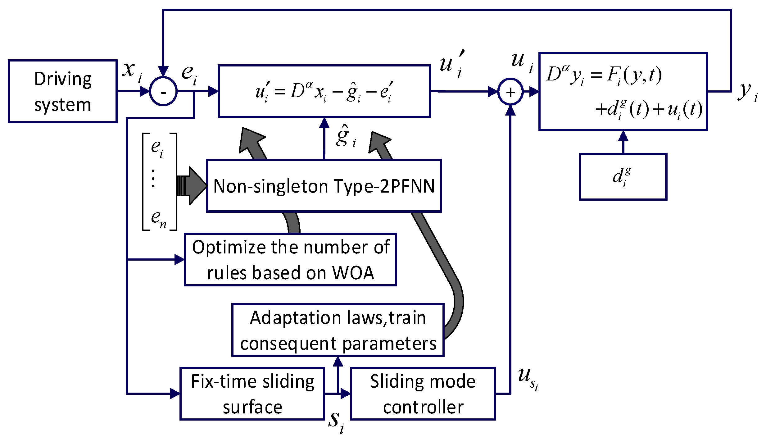
The i-th subsystem is defined as follows:

$$D^{\alpha }{y}_i=F_i(y,t)+d_i^g(t)+u_i(t),$$

(8)

where $F_i(y,t)=g_i(y,t)+\Delta g_i(y,t)$ as shown in Figure 1, and $({\widehat{g}}_i)$ is estimated using the proposed NST2PFNN.

Set

$$F_i(y,t)=g_i^{\ast }+{\epsilon }_i,$$

(9)

where ${\epsilon }_i$ is the estimation error ($\left|{\epsilon }_i\right|\le {\epsilon }^{\ast }$), and $g_i^{\ast }$ is the best estimated value ($\left|g_i^{\ast }\right|\le {\epsilon }_{g^{\ast }}$).

The control law is defined as follows:

$$u_i={u^{\prime }}_i+u_{s_i},$$

(10)

$${u^{\prime }}_i=D^{\alpha }{x}_i-{\widehat{g}}_i-{e^{\prime }}_i,$$

(11)

where ${e^{\prime }}_i=D^{\alpha -1}({\beta }_1{(1/2)}^{m_1/n_1}sig{(e_i)}^{2m_1/n_1-1}+{\lambda }_1{(1/2)}^{p_1/q_1}sig{(e_i)}^{2p_1/q_1-1})$; $D^{\alpha }$ is the fractional differential operator with order $\alpha$, ${\beta }_1>0$, and ${\lambda }_1>0$; $m_1$, $n_1$, $p_1$, and $q_1$ are positive odd integers with $m_1>n_1$ and $p_1<q_1$; and ${\widehat{g}}_i$ is the bounded output of SENSIT2PFNN with $\left|{\widehat{g}}_i\right|\le {\epsilon }_{\widehat{g}}$.

The i-th error subsystem can be obtained by using Equations (9)–(11):

$$D^{\alpha }{e}_i=g_i^{\ast }+{\epsilon }_i-{\widehat{g}}_i-{e^{\prime }}_i+u_{s_i}+d_i^g.$$

(12)

We aimed to design a fixed-time sliding mode control law ($u_{s_i}$) such that the error system given by Equation (12) can become stable within a fixed period independent of the initial value.

3. Self-Evolving Non-Singleton Type-2 Probabilistic Fuzzy Neural Network

3.1. Network Structure

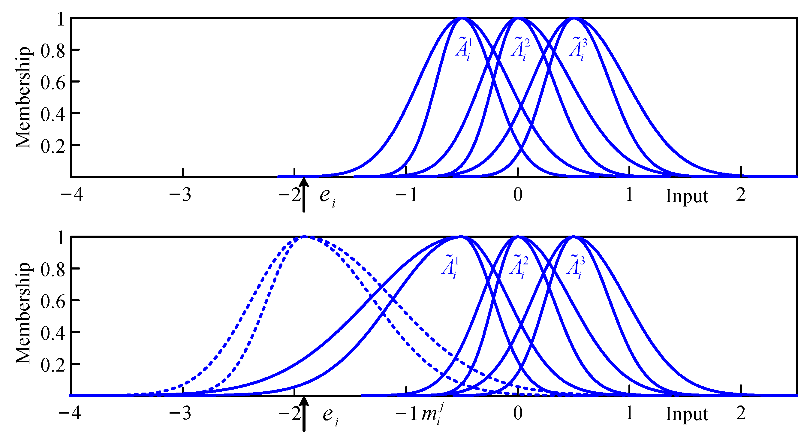
To facilitate the self-evolution of the membership layer structure presented, type-2 asymmetric Gaussian functions are employed as the activation functions of all the neural network layers because they offer good flexibility. As shown in Figure 2, the NSIT2PFNN model has six layers:

Input layer: The input of this layer is the output of the error system.

Fuzzification layer: In this layer, the single point input of the neural network is fuzzified into a type-2 membership function (MF), representing the uncertainty of the input. Let the type-2 MF generated by the i-th input be ${\tilde{B}}_{e_i}$. ${\tilde{B}}_{e_i}$ utilizes an asymmetric Gaussian MF with a mean value of $e_i$ and a standard deviation width of ${\sigma }_{e_i}^L\in [{\underset{\_}{\sigma }}_{e_i}^L,{\overline{\sigma }}_{e_i}^L]$–${\sigma }_{e_i}^R\in [{\underset{\_}{\sigma }}_{e_i}^R,{\overline{\sigma }}_{e_i}^R]$:

$$\begin{array}{l}{\overline{\mu }}_{{\tilde{B}}_{e_i}}(x)=\{\begin{array}{l}\exp (-\frac{{(x-e_i)}^2}{{\overline{\sigma }}_{e_i}^{L2}}),-\infty <x\le e_i\\ \exp (-\frac{{(x-e_i)}^2}{{\overline{\sigma }}_{e_i}^{R2}}),e_i<x\le \infty \end{array}\\ {\underset{\_}{\mu }}_{{\tilde{B}}_{e_i}}(x)=\{\begin{array}{l}\exp (-\frac{{(x-e_i)}^2}{{\underset{\_}{\sigma }}_{e_i}^{L2}}),-\infty <x\le e_i\\ \exp (-\frac{{(x-e_i)}^2}{{\underset{\_}{\sigma }}_{e_i}^{R2}}),e_i<x\le \infty \end{array}\end{array}.$$

(13)

As shown in Figure 3, to obtain the upper and lower membership degrees of the i-th input of the network under the j-th MF, the input of the network must be non-singleton blurred [40]:

$$\begin{array}{l}{\overline{e}}_i^j=\{\begin{array}{l}\frac{[{({\overline{\sigma }}_i^{Lj})}^2{e}_i+{({\overline{\sigma }}_{e_i}^R)}^2{m}_i^j]}{[{({\overline{\sigma }}_i^{Lj})}^2+{({\overline{\sigma }}_{e_i}^R)}^2]},e_i\le m_i^j\\ \frac{[{({\overline{\sigma }}_i^{Rj})}^2{e}_i+{({\overline{\sigma }}_{e_i}^L)}^2{m}_i^j]}{[{({\overline{\sigma }}_i^{Rj})}^2+{({\overline{\sigma }}_{e_i}^L)}^2]},e_i>m_i^j\end{array}\\ {\underset{\_}{e}}_i^j=\{\begin{array}{l}\frac{[{({\underset{\_}{\sigma }}_i^{Lj})}^2{e}_i+{({\underset{\_}{\sigma }}_{e_i}^R)}^2{m}_i^j]}{[{({\underset{\_}{\sigma }}_i^{Lj})}^2+{({\underset{\_}{\sigma }}_{e_i}^R)}^2]},e_i\le m_i^j\\ \frac{[{({\underset{\_}{\sigma }}_i^{Rj})}^2{e}_i+{({\underset{\_}{\sigma }}_{e_i}^L)}^2{m}_i^j]}{[{({\underset{\_}{\sigma }}_i^{Rj})}^2+{({\underset{\_}{\sigma }}_{e_i}^L)}^2]},e_i>m_i^j\end{array}\end{array},$$

(14)

where $j=1,\dots ,K$; $m_i^j$ ${\sigma }_i^{Lj}$, and ${\sigma }_i^{Rj}$ are, respectively, the mean and standard deviations of the j-th type-2 MF$({\tilde{A}}_i^j)$ of the i-th input; and $e_i^j$ is the fuzzy value of the i-th input under the j-th MF.

Membership layer: The membership degree of the i-th input under the j-th MF is calculated in this layer:

$$\begin{array}{l}{\overline{\mu }}_{{\tilde{A}}_i^j}({\overline{e}}_i^j)=\{\begin{array}{l}\exp [-\frac{{({\overline{e}}_i^j-m_i^j)}^2}{{\overline{\sigma }}_i^{Lj2}}],{\overline{e}}_i^j\le m_i^j\\ \exp [-\frac{{({\overline{e}}_i^j-m_i^j)}^2}{{\overline{\sigma }}_i^{Rj2}}],{\overline{e}}_i^j>m_i^j\end{array}\\ {\underset{\_}{\mu }}_{{\tilde{A}}_i^j}({\underset{\_}{e}}_i^j)=\{\begin{array}{l}\exp [-\frac{{({\underset{\_}{e}}_i^j-m_i^j)}^2}{{\underset{\_}{\sigma }}_i^{Lj2}}],{\underset{\_}{e}}_i^j\le m_i^j\\ \exp [-\frac{{({\underset{\_}{e}}_i^j-m_i^j)}^2}{{\underset{\_}{\sigma }}_i^{Rj2}}],{\underset{\_}{e}}_i^j>m_i^j\end{array}\end{array},$$

(15)

where ${\tilde{A}}_i^j$ is the j-th MF of the i-th input; ${\overline{\mu }}_{{\tilde{A}}_i^j}$ and ${\underset{\_}{\mu }}_{{\tilde{A}}_i^j}$ are, respectively, the upper and lower membership degrees of the i-th input under the j-th MF; and ${\sigma }_i^{Lj}$ and ${\sigma }_i^{Rj}$ are, respectively the left and right width of the MF.

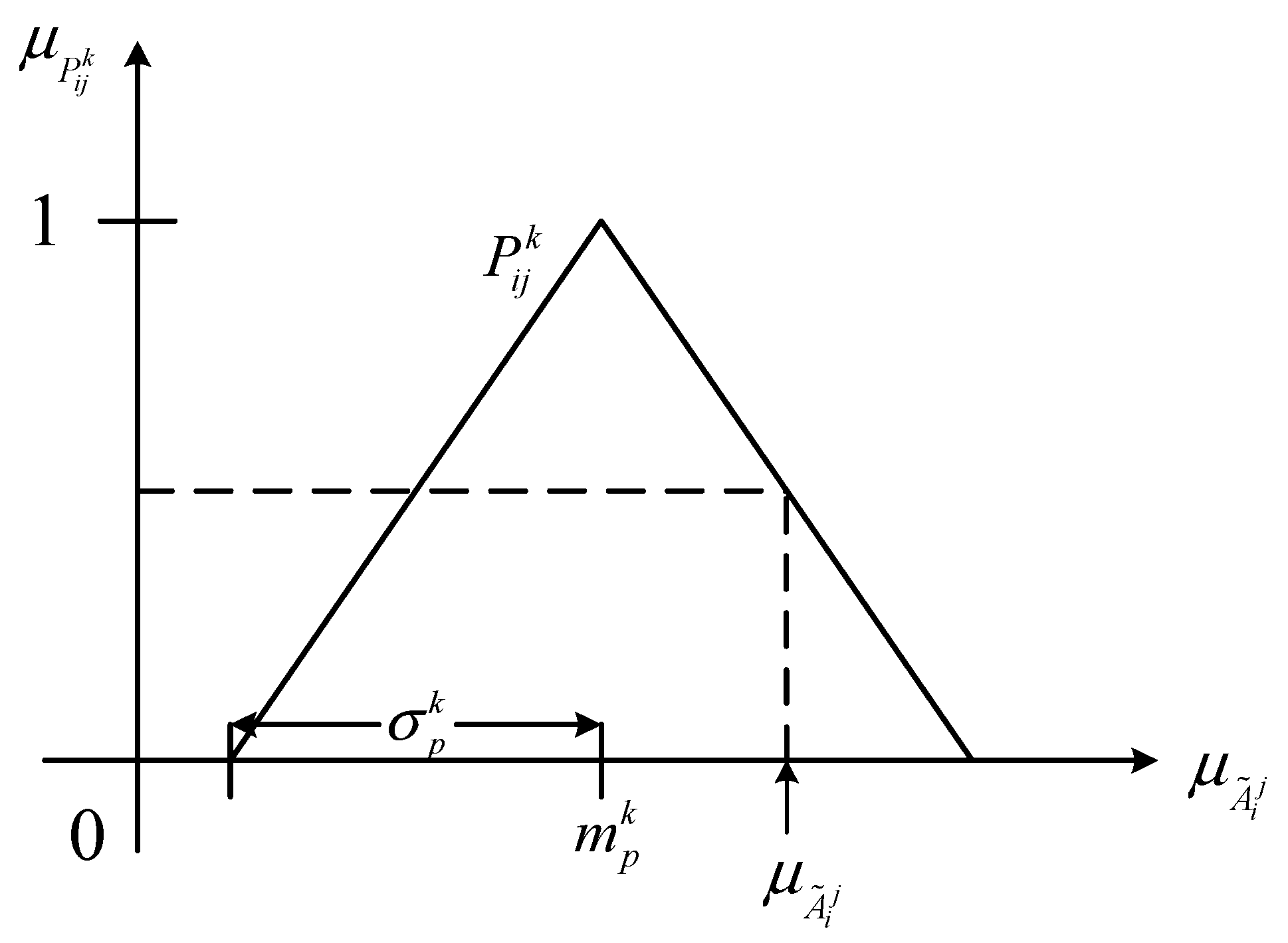
Probabilistic layer: In this layer, the Gaussian function is usually employed as the probability function (PF). To improve calculation efficiency, as shown in Figure 4, the triangle function was used in this study:

$$\begin{array}{l}{\overline{\mu }}_{P_{ij}^k}({\overline{\mu }}_{{\tilde{A}}_i^j})=\{\begin{array}{l}0,{\overline{\mu }}_{{\tilde{A}}_i^j}\ge m_p^k+{\sigma }_p^k,{\overline{\mu }}_{{\tilde{A}}_i^j}\le m_p^k-{\sigma }_p^k\\ \frac{{\overline{\mu }}_{{\tilde{A}}_i^j}-m_p^k+{\sigma }_p^k}{{\sigma }_p^k},m_p^k-{\sigma }_p^k<{\overline{\mu }}_{{\tilde{A}}_i^j}\le m_p^k\\ \frac{-{\overline{\mu }}_{{\tilde{A}}_i^j}+m_p^k+{\sigma }_p^k}{{\sigma }_p^k},m_p^k<{\overline{\mu }}_{{\tilde{A}}_i^j}\le m_p^k+{\sigma }_p^k\end{array}\\ {\underset{\_}{\mu }}_{P_{ij}^k}({\overline{\mu }}_{{\tilde{A}}_i^j})=\{\begin{array}{l}0,{\underset{\_}{\mu }}_{{\tilde{A}}_i^j}\ge m_p^k+{\sigma }_p^k,{\underset{\_}{\mu }}_{{\tilde{A}}_i^j}\le m_p^k-{\sigma }_p^k\\ \frac{{\underset{\_}{\mu }}_{{\tilde{A}}_i^j}-m_p^k+{\sigma }_p^k}{{\sigma }_p^k},m_p^k-{\sigma }_p^k<{\underset{\_}{\mu }}_{{\tilde{A}}_i^j}\le m_p^k\\ \frac{-{\underset{\_}{\mu }}_{{\tilde{A}}_i^j}+m_p^k+{\sigma }_p^k}{{\sigma }_p^k},m_p^k<{\underset{\_}{\mu }}_{{\tilde{A}}_i^j}\le m_p^k+{\sigma }_p^k\end{array}\end{array},$$

(16)

where $P_{ij}^k$ is the k-th PF of the j-th MF, ${\overline{\mu }}_{P_{ij}^k}$ and ${\underset{\_}{\mu }}_{P_{ij}^k}$ are the output of the k-th node of the j-th input variable, $m_p^k$ is the center of the triangle, and ${\sigma }_p^k$ is the center width of the triangle.

Rule layer: Each node in this layer represents a fuzzy rule, which calculates the upper and lower firing degrees based on product reasoning. Each rule is defined as follows:

$$Rul{e}^l: \mathrm{IF} e_1 \mathrm{is} {\tilde{A}}_1^{P_1} \mathrm{and} \dots \mathrm{and} e_n \mathrm{is} {\tilde{A}}_n^{P_n},\mathrm{then} \widehat{g} \mathrm{is} {\omega }^l,$$

(17)

where ${\tilde{A}}_i^{P_j}$ is the p_j-th type-2 MF of the i-th input, and ${\omega }^l$ is the consequent parameter of the l-th rule. Let the total number of rules be M, and the upper and lower firing degrees of the l-th rule are

$$\begin{array}{l}{\overline{z}}^l=({\overline{\mu }}_{{\tilde{A}}_i^j}\times \underset{k}{\Pi }{\overline{\mu }}_{P_{ij}^k})\times \cdots \times ({\overline{\mu }}_{{\tilde{A}}_n^K}\times \underset{k}{\Pi }{\overline{\mu }}_{P_{nK}^k})\\ {\underset{\_}{z}}^l=({\underset{\_}{\mu }}_{{\tilde{A}}_i^j}\times \underset{k}{\Pi }{\underset{\_}{\mu }}_{P_{ij}^k})\times \cdots \times ({\underset{\_}{\mu }}_{{\tilde{A}}_n^K}\times \underset{k}{\Pi }{\underset{\_}{\mu }}_{P_{nK}^k})\end{array},$$

(18)

where ${\overline{z}}^l$ and ${\underset{\_}{z}}^l$ are, respectively, the upper and lower firing degrees of the l-th rule, and K is the number of MFs per network input.

Output layer: The output of deblurring can be expressed as follows:

$$\widehat{g}=\frac{{\displaystyle \sum _{i=1}^M({\underset{\_}{z}}^i+{\overline{z}}^i){\omega }^i}}{{\displaystyle \sum _{i=1}^M({\underset{\_}{z}}^i+{\overline{z}}^i)}}.$$

(19)

To facilitate the subsequent derivation process, $\widehat{g}$ can be written as follows:

$$\begin{array}{l}H=\frac{1}{{\displaystyle \sum _{i=1}^M({\underset{\_}{z}}^i+{\overline{z}}^i)}}{\left[\left({\underset{\_}{z}}^1+{\overline{z}}^1\right)\cdots \left({\underset{\_}{z}}^M+{\overline{z}}^M\right)\right]}^{{\rm T}}\\ W_i={\left[{\omega }_i{}^1\cdots {\omega }_i{}^M\right]}^{{\rm T}},{\tilde{W}}_i=W_i^{\ast }-{\widehat{W}}_i\\ {\widehat{g}}_i={\widehat{W}}_i{}^{{\rm T}}H,g_i^{\ast }=W_i^{\ast {\rm T}}H\end{array},$$

(20)

where $W_i$ is the weight vector of the i-th neural network, $W_i^{\ast }$ is the optimal estimate of the weight, and ${\widehat{W}}_i$ is the weight estimate.

3.2. Self-Evolution Algorithm

(1)

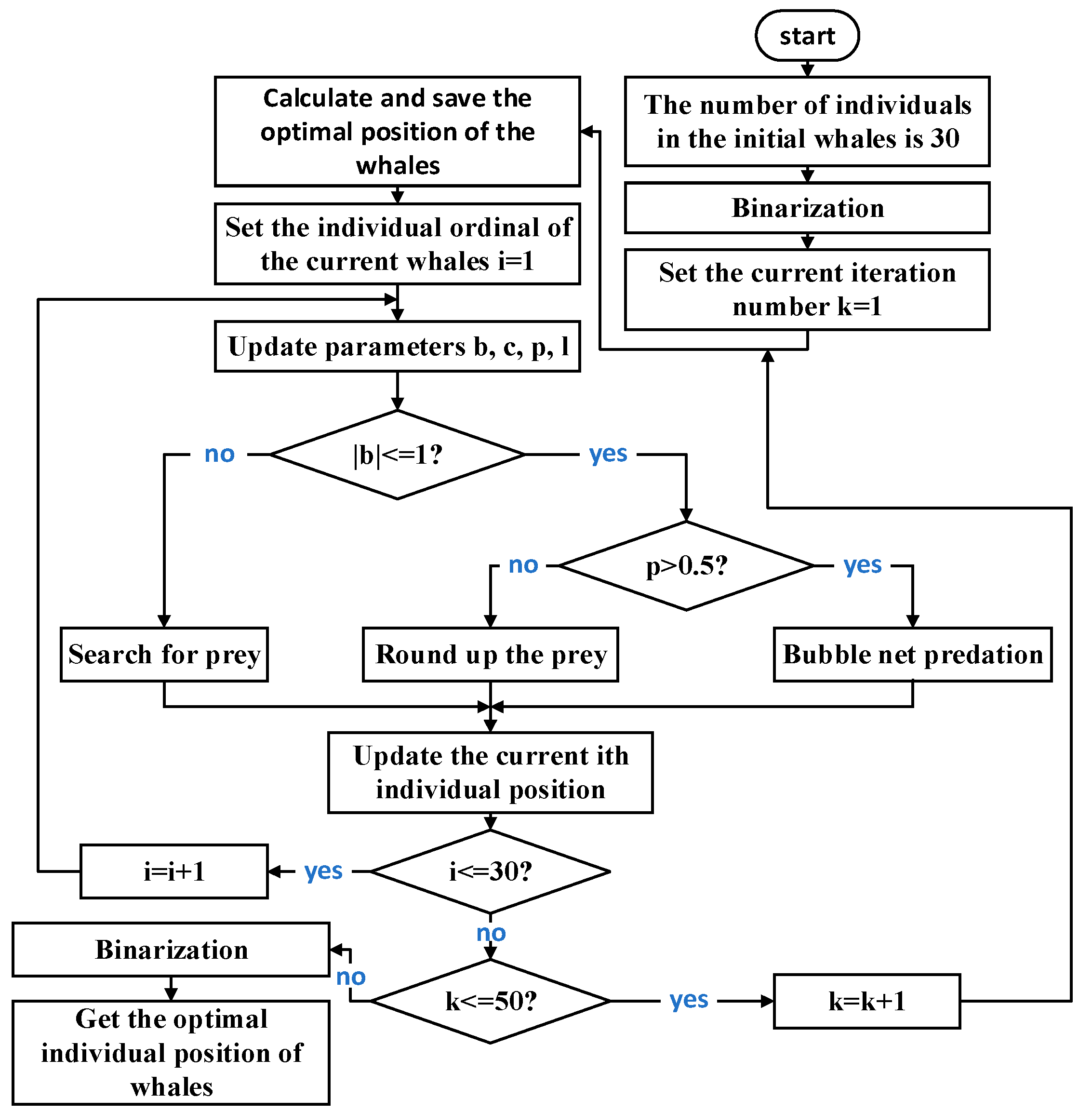
Optimizing the rule base of neural networks with the improved WOA.

Due to the curse of dimensionality, an FNN with $n$ inputs and $K$ membership functions for each input generates up to $K^n$ rules, which greatly increases unnecessary calculations. WOA offers the advantages of simple mechanisms, few parameters, and strong optimization ability. To make WOA suitable for the optimization of the NSIT2PFNN rule base, it was modified appropriately in this study; the steps are shown in Figure 5.

First, the total number of rules M of the network was obtained, and the individual position vector of the population with dimension M was randomly generated. Next, the population size was set as 30 and binarized (set as 0 if it was less than 0.5 and as 1 for the rest). Each position was multiplied with the neural network rules to calculate the optimal fitness value for the current optimal individual position. The basic parameters, such as $b$ and $p$, were initialized such that when $\left|b\right|\le 1$ and $p\le 0.5$, the individual population updates its position by following the “round up the prey” strategy; when $\left|b\right|\le 1$ and $p>0.5$, the individual population updates its position by following the “bubble net predation” strategy; and when $\left|b\right|>1$, the individual population updates its position by following the “search for prey” strategy. After a round of position updates was completed, all position information was brought into the neural network rule base, the fitness value was calculated, the optimal individual position was retained, and the cycle was terminated upon reaching the maximum number of iterations. In this paper, the maximum number of iterations was set as 50, and the following fitness function was used:

$$J={\displaystyle {\int }_0^{\infty }{\displaystyle \sum _{i=1}^n\left|e_i(t)\right|}}dt.$$

(21)

Remark 1.

In this paper, only two numbers were used in the individual coordinate values of the population to be optimized: 0 and 1. In such cases, the traditional WOA is no longer applicable, and all population individuals and the search space must be binarized after each iteration to generate a new population. The binarization algorithm can be expressed as follows:

$$a_i(t)=\{\begin{array}{c}1\begin{array}{ccc}& & round(a_i(t))\%2=1\end{array}\\ 0\begin{array}{ccc}& & round(a_i(t))\%2=0\end{array}\end{array},$$

(22)

where $a_i(t)$ is the i-th coordinate value of an individual in the population.

(2)

Self-evolution of the membership layer of NSIT2PFNN

The structure of the membership layer of NSIT2PFNN was optimized by considering the following three type-2 MFs of the i-th input: ${\tilde{A}}_i^1({\sigma }_i^{L1},m_i^1,{\sigma }_i^{R1})$, ${\tilde{A}}_i^2({\sigma }_i^{L2},m_i^2,{\sigma }_i^{R2})$, and ${\tilde{A}}_i^3({\sigma }_i^{L3},m_i^3,{\sigma }_i^{R3})$, where ${\sigma }_i^{Lj}\in [{\overline{\sigma }}_i^{Lj},{\underset{\_}{\sigma }}_i^{Lj}],j=1,2,3$ is the left width of the standard deviation of the MF, $m_i^j,j=1,2,3$ is the mean point of the MF, ${\sigma }_i^{Rj}\in [{\overline{\sigma }}_i^{Rj},{\underset{\_}{\sigma }}_i^{Rj}],j=1,2,3$ is the right width of the standard deviation of the MF, and the standard deviation width of each input of lower MF is half of that of the upper MF. As shown in Figure 6, for each input $e_i$, if the maximum upper membership degree is lower than the set value min_Degree (0.2), a new type-2 MF is generated. Its mean point is $e_i$, and the width of the left (right) standard deviation is the distance from its mean point to the mean point of the adjacent MF:

$$\{\begin{array}{l}{\overline{\sigma }}_{e_i}^{Rj}=m_i^1-e_i\\ {\overline{\sigma }}_{e_i}^{Lj}=e_i-m_i^3\end{array}.$$

(23)

The right (left) standard deviation width of its adjacent MF was changed in the same manner.

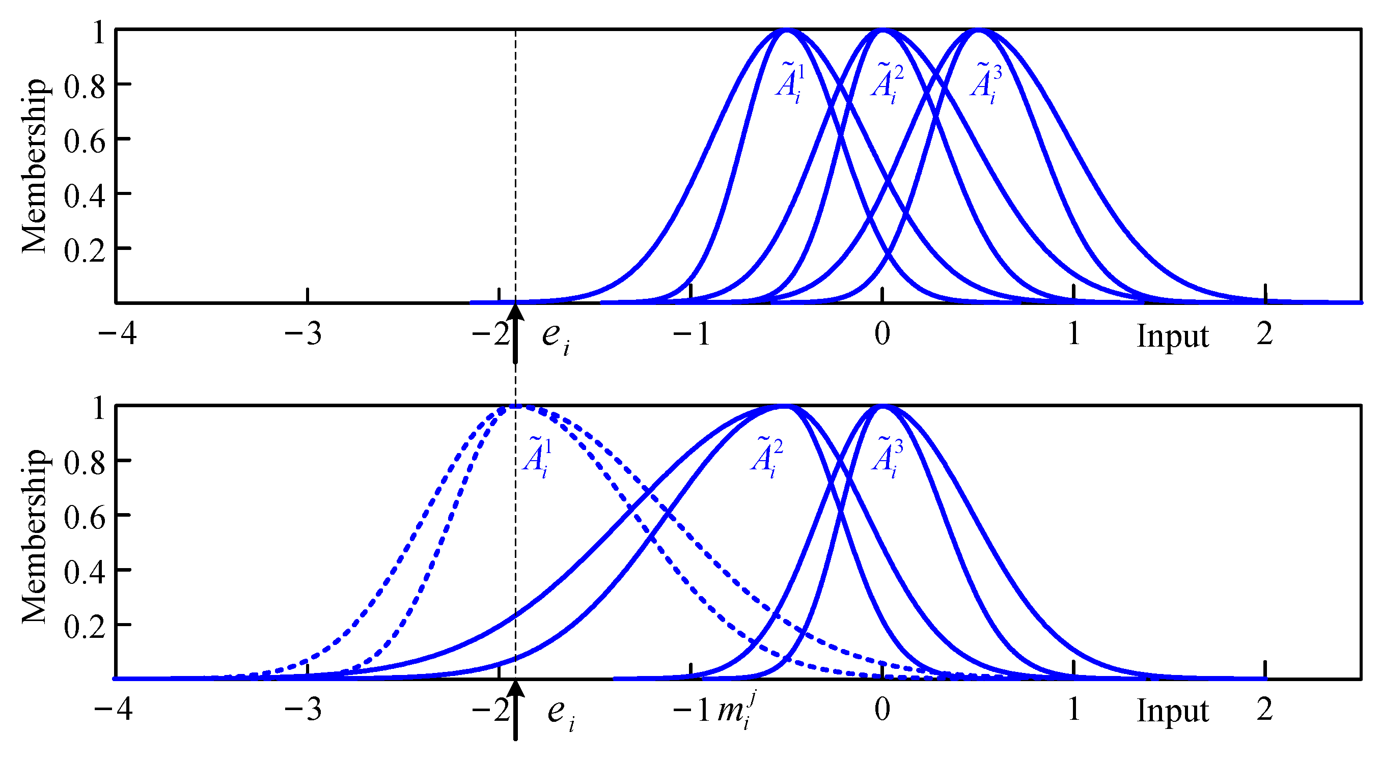
If the number of MFs exceeds the set value max_Mf (value 3), the farthest MF is deleted, as shown in Figure 7.

4. Controller Design and Stability Analysis

We designed a fixed-time sliding mode controller $u_{s_i}$ to stabilize the error subsystem given by Equation (12). The sliding surface can be selected as follows:

$$\begin{array}{cc}\hfill s_i& =D^{\alpha -1}{e}_i+D^{\alpha -2}({\beta }_1{(1/2)}^{m_1/n_1}sig{(e_i)}^{2m_1/n_1-1}\hfill \\ & +{\lambda }_1{(1/2)}^{p_1/q_1}sig{(e_i)}^{2p_1/q_1-1})\hfill \end{array},$$

(24)

where $s_i$ is the sliding surface of the i-th subsystem; ${\beta }_1>0$; ${\lambda }_1>0$; $m_1$, $n_1$, $p_1$, and $q_1$ are positive odd integers such that $m_1>n_1$ and $p_1<q_1$; and $sig{(\cdot )}^x={|\cdot |}^{x}sig(\cdot )$.

When the state variable of the error system reaches the sliding surface, it satisfies the following condition:

$$\begin{array}{c}{D}^{\alpha -1}{e}_i=-D^{\alpha -2}({\beta }_1{(1/2)}^{m_1/n_1}sig{(e_i)}^{2m_1/n_1-1}\\ +{\lambda }_1{(1/2)}^{p_1/q_1}sig{(e_i)}^{2p_1/q_1-1})\end{array}.$$

(25)

Theorem 1.

The state variable of the error subsystem given by Equation (12) converges to zero within a fixed time $T_1$ after reaching the sliding surface:

$$T_1<\frac{1}{n^{1-m_1/n_1}{\beta }_1}\frac{n_1}{m_1-n_1}+\frac{1}{{\lambda }_1}\frac{q_1}{q_1-p_1}.$$

(26)

Proof. 

According to the Lyapunov function:

$$V_1(t)=\frac{1}{2}{\displaystyle \sum _{i=1}^n{e}_i^2}.$$

(27)

According to Property 1, the derivative of the Lyapunov function with respect to time t can be obtained as follows:

$$\begin{array}{cc}\hfill {\dot{V}}_1& ={\displaystyle \sum _{i=1}^n{e}_i{\dot{e}}_i}\hfill \\ & ={\displaystyle \sum _{i=1}^n{e}_i(D^{2-\alpha }(D^{\alpha -1}{e}_i))}\hfill \\ & =-{\displaystyle \sum _{i=1}^n({\beta }_1{(\frac{1}{2}{e}_i^2)}^{m_1/n_1}+{\lambda }_1{(\frac{1}{2}{e}_i^2)}^{p_1/q_1})}\hfill \end{array}.$$

(28)

According to Lemma 2:

$$\begin{array}{cc}\hfill {\dot{V}}_1& \le -n^{1-m_1/n_1}{\beta }_1{(\frac{1}{2}{\displaystyle \sum _{i=1}^n{e}_i^2})}^{m_1/n_1}-{\lambda }_1{(\frac{1}{2}{\displaystyle \sum _{i=1}^n{e}_i^2})}^{p_1/q_1}\hfill \\ & =-n^{1-m_1/n_1}{\beta }_1{V}_1{}^{m_1/n_1}-{\lambda }_1{V}_1{}^{p_1/q_1}\hfill \end{array}.$$

(29)

According to Lemma 1, the state variable of the error subsystem converges to zero within a fixed time $T_1$ after reaching the sliding surface. Thus, Theorem 1 is proved.

The sliding mode control law $u_{s_i}$ can be designed as follows:

$$\begin{array}{cc}{u}_{s_i}& =-{\beta }_2{(1/2)}^{m_2/n_2}sig{(s_i)}^{2m_2/n_2-1}\hfill \\ & -{\lambda }_2{(1/2)}^{p_2/q_2}sig{(s_i)}^{2p_2/q_2-1}-{\eta }_{i}sig(s_i)\hfill \end{array}.$$

(30)

Then:

$$\begin{array}{cc}\hfill u_i& ={u^{\prime }}_i+u_{s_i}\hfill \\ & =D^{\alpha }{x}_i-{\widehat{g}}_i-e^{\prime }-{\beta }_2{(1/2)}^{m_2/n_2}sig{(s_i)}^{2m_2/n_2-1}\hfill \\ & -{\lambda }_2{(1/2)}^{p_2/q_2}sig{(s_i)}^{2p_2/q_2-1}-{\eta }_{i}sig(s_i)\hfill \end{array}.$$

(31)

□

Theorem 2.

The error subsystem given by Equation (12) converges to the sliding mode surface $s_i$ under the control law (Equation (31)).

Proof. 

According to the Lyapunov function:

$$V_2={\displaystyle \sum _{i=1}^n(\frac{1}{2}{s}_i^2+\frac{1}{2}{\tilde{W}}_i^{{\rm T}}{\tilde{W}}_i)}.$$

(32)

According to Equation (20), the derivative of the Lyapunov function with respect to time $t$ is obtained as follows:

$${\dot{V}}_2={\displaystyle \sum _{i=1}^n(s_i{\dot{s}}_i-{\tilde{W}}_i^{{\rm T}}{\dot{\widehat{W}}}_i)}.$$

(33)

Substituting Equations (12), (20), and (24) into Equation (33), we obtain:

$$\begin{array}{cc}\hfill {\dot{V}}_2& ={\displaystyle \sum _{i=1}^n(s_i(D^{\alpha }{e}_i+{e^{\prime }}_i)-{\tilde{W}}_i^{{\rm T}}{\dot{\widehat{W}}}_i)}\hfill \\ & ={\displaystyle \sum _{i=1}^n(s_i(g_i^{\ast }+{\epsilon }_i-{\widehat{g}}_i-{e^{\prime }}_i+u_{s_i}+d_i^g+{e^{\prime }}_i)-{\tilde{W}}_i^{{\rm T}}{\dot{\widehat{W}}}_i)}\hfill \\ & ={\displaystyle \sum _{i=1}^n(s_i(W_i^{\ast {\rm T}}H+{\epsilon }_i-{\widehat{W}}_i^{{\rm T}}H+u_{s_i}+d_i^g)-{\tilde{W}}_i^{{\rm T}}\dot{\widehat{W}})}\hfill \end{array}.$$

(34)

Setting $\dot{\widehat{W}}=s_{i}H$, we obtain:

$$\begin{array}{cc}\hfill {\dot{V}}_2& ={\displaystyle \sum _{i=1}^n{s}_i({\epsilon }_i-{\beta }_2{(1/2)}^{m_2/n_2}sig{(s_i)}^{2m_2/n_2-1}}\hfill \\ & -{\lambda }_2{(1/2)}^{p_2/q_2}sig{(s_i)}^{2p_2/q_2-1}-{\eta }_{i}sig(s_i)+d_i^g)\hfill \\ & ={\displaystyle \sum _{i=1}^n(s_i{\epsilon }_i-{\beta }_2{(\frac{1}{2}{s}_i^2)}^{m_2/n_2}}\hfill \\ & -{\lambda }_2{(\frac{1}{2}{s}_i^2)}^{p_2/q_2}-\eta \left|s_i\right|+s_i{d}_i^g)\hfill \end{array}.$$

(35)

Setting ${\eta }_i>{\epsilon }^{\ast }+{\epsilon }_d+{\epsilon }_{\widehat{g}}+{\epsilon }_{g^{\ast }}$, we obtain:

$${\dot{V}}_2\le {\displaystyle \sum _{i=1}^n(-{\beta }_2{(\frac{1}{2}{s}_i^2)}^{m_2/n_2}-{\lambda }_2{(\frac{1}{2}{s}_i^2)}^{p_2/q_2})}\le 0.$$

(36)

Thus, according to the Lyapunov stability theorem, Theorem 2 is proved. □

Theorem 3.

The error subsystem given by Equation (12) converges to the sliding mode surface $s_i$ within a fixed time $t$ under the action of the control law (Equation (31)):

$$T_2<\frac{1}{n^{1-m_2/n_2}{\beta }_2}\frac{n_2}{m_2-n_2}+\frac{1}{{\lambda }_2}\frac{q_2}{q_2-p_2}.$$

(37)

Proof. 

According to the Lyapunov function:

$$V_3(t)=\frac{1}{2}{\displaystyle \sum _{i=1}^n{s}_i^2}.$$

(38)

Substituting Equations (12) and (24) into Equation (38) and differentiating it, we obtain:

$$\begin{array}{cc}\hfill V_3(t)& ={\displaystyle \sum _{i=1}^n{s}_i{\dot{s}}_i}={\displaystyle \sum _{i=1}^n{s}_i(D^{\alpha }{e}_i+{e^{\prime }}_i)}\hfill \\ & ={\displaystyle \sum _{i=1}^n{s}_i(g_i^{\ast }+{\epsilon }_i-{\widehat{g}}_i-{e^{\prime }}_i+u_{s_i}+d_i^g+{e^{\prime }}_i)}\hfill \\ & ={\displaystyle \sum _{i=1}^n{s}_i(g_i^{\ast }+{\epsilon }_i-{\widehat{g}}_i-{\beta }_2{(1/2)}^{m_2/n_2}sig{(s_i)}^{2m_2/n_2-1}}\hfill \\ & -{\lambda }_2{(1/2)}^{p_2/q_2}sig{(s_i)}^{2p_2/q_2-1}-{\eta }_{i}sig(s_i)+d_i^g)\hfill \end{array}.$$

(39)

Setting ${\eta }_i>{\epsilon }^{\ast }+{\epsilon }_d+{\epsilon }_{\widehat{g}}+{\epsilon }_{g^{\ast }}$, we obtain:

$$V_3(t)\le {\displaystyle \sum _{i=1}^n(-{\beta }_2{(\frac{1}{2}{s}_i^2)}^{m_2/n_2}-{\lambda }_2{(\frac{1}{2}{s}_i^2)}^{p_2/q_2})}.$$

(40)

According to Lemma 2:

$$\begin{array}{cc}\hfill {\dot{V}}_3& \le -n^{1-m_2/n_2}{\beta }_2{(\frac{1}{2}{\displaystyle \sum _{i=1}^n{s}_i^2})}^{m_2/n_2}-{\lambda }_2{(\frac{1}{2}{\displaystyle \sum _{i=1}^n{s}_i^2})}^{p_2/q_2}\hfill \\ & =-n^{1-m_2/n_2}{\beta }_2{V}_3{}^{m_2/n_2}-{\lambda }_2{V}_3{}^{p_2/q_2}\hfill \end{array}.$$

(41)

According to Lemma 1, the error subsystem converges to the sliding mode surface $s_i$ within a fixed time $T_2$ under the action of control law (Equation (31)). Thus, Theorem 3 is proved. □

5. Simulation

We verified the effectiveness of the proposed fractional-order hyperchaotic system synchronization scheme by performing simulation experiments.

As performed in a previous study [41], we used the fractional-order hyperchaotic Chen system as the drive system and the fractional-order hyperchaotic Lorenz system as the response system. The respective formulas are as follows:

$$\mathrm{Drive} \mathrm{system}: \{\begin{array}{l}{D}^{\alpha }{x}_1=35(x_2-x_1)+x_4\\ D^{\alpha }{x}_2=7x_1+12x_2-x_1{x}_3\\ D^{\alpha }{x}_3=x_1{x}_2-8x_3\\ D^{\alpha }{x}_4=x_2{x}_3+0.3x_4\end{array},$$

(42)

$$\mathrm{Response} \mathrm{system}: \{\begin{array}{l}{D}^{\alpha }{y}_1=10(y_2-y_1)+y_4+\Delta g_1+d_1^y+u_1\\ D^{\alpha }{y}_2=28y_1-y_2-y_1{y}_3+\Delta g_2+d_2^y+u_2\\ D^{\alpha }{y}_3=y_1{y}_2-8/3y_3+\Delta g_3+d_3^y+u_3\\ D^{\alpha }{y}_4=-y_2{y}_3-y_4+\Delta g_4+d_4^y+u_4\end{array},$$

(43)

where the nonlinear unknown function $\Delta g_i$ and external interference $d_i^y$ are selected as follows:

$$\begin{array}{l}\Delta g_1+d_1^y=0.25\cos (6t)y_1-0.15\sin (t)\\ \Delta g_2+d_2^y=-0.2\cos (2t)y_2+0.1\sin (3t)\\ \Delta g_3+d_3^y=0.15\sin (3t)y_3+0.2\cos (5t)\\ \Delta g_4+d_4^y=-0.2\cos (t)y_4-0.15\cos (t)\end{array}.$$

(44)

The proposed method was used for synchronization control. The parameters of NSIT2PFNN are presented in

Table 1. Initial parameters of NSIT2PFNN.

Initial Parameters of MF									Initial Parameters of PF
$A_i^1$			$A_i^2$			$A_i^3$			$P_{ij}^1$		$P_{ij}^2$		$P_{ij}^3$
${\sigma }_i^{L1}$	$m_i^1$	${\sigma }_i^{R1}$	${\sigma }_i^{L2}$	$m_i^2$	${\sigma }_i^{R2}$	${\sigma }_i^{L3}$	$m_i^3$	${\sigma }_i^{R3}$	${\sigma }_p^1$	$m_p^1$	${\sigma }_p^2$	$m_p^2$	${\sigma }_p^3$	$m_p^3$
−20	−10	0	−10	0	10	0	10	20	1	0.4	1	0.5	1	0.6

. The initial values were set as follows:

$[x_1(0),x_2(0),x_3(0),x_4(0)]$$=$$[3,1,4,-1]$, and $[y_1(0),y_2(0),y_3(0),y_4(0)]$=$[1,2,3,4]$, with the fractional order $\alpha =0.98$. The control parameters were set as ${\eta }_i=8$, ${\beta }_1={\beta }_2=12$, ${\lambda }_1={\lambda }_2=12$, $p_1=p_2=5$, $q_1=q_2=9$, $n_1=n_2=5$, and $m_1=m_2=9$.

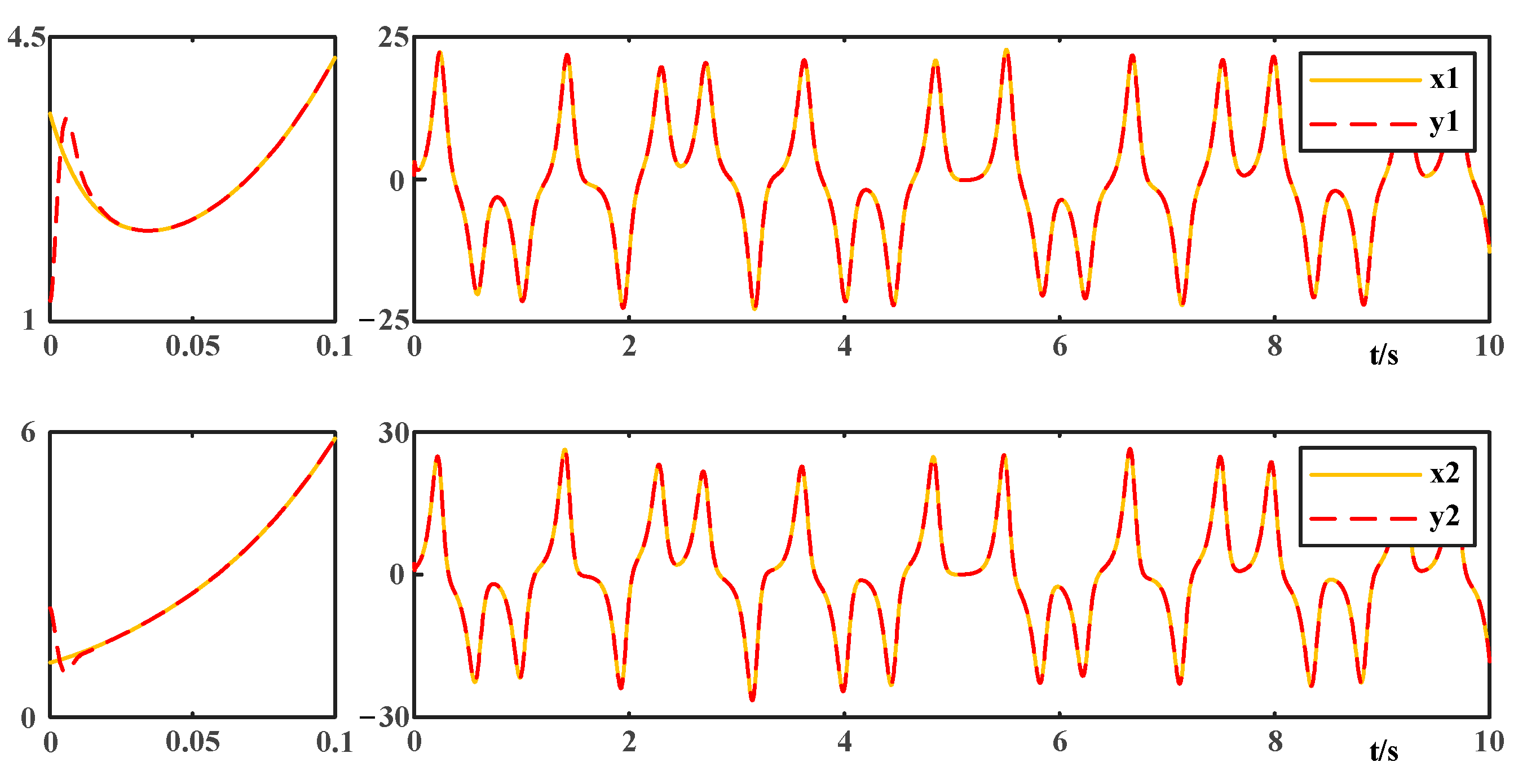
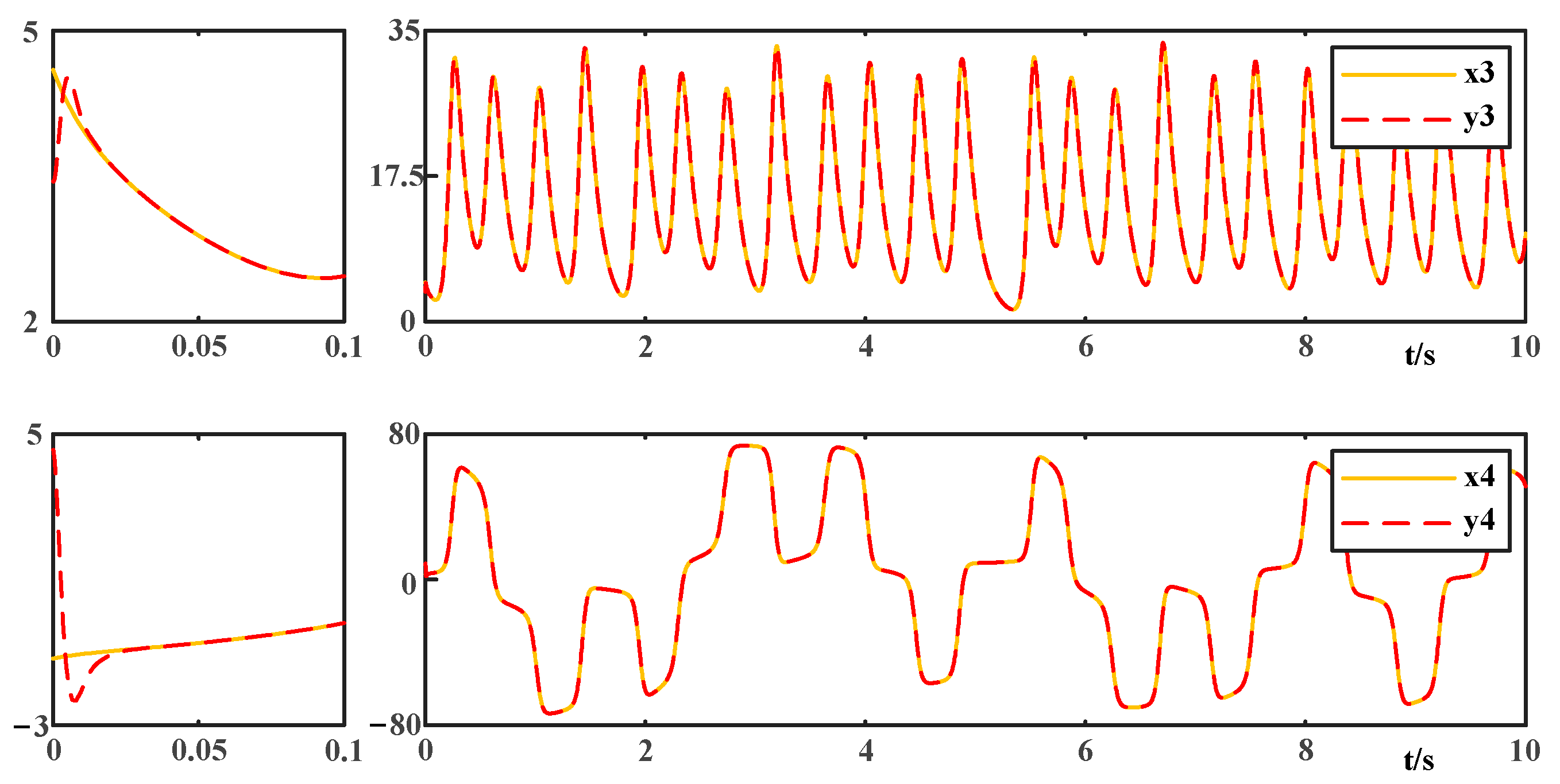
The synchronization results are shown in Figure 8 and Figure 9, and the root mean square error (RMSE) values are presented in

Table 2. RMSE values of the proposed and other methods proposed in the literature [41,42,43].

	RMSE
	${\mathit{e}}_1$	${\mathit{e}}_2$	${\mathit{e}}_3$	${\mathit{e}}_4$
Proposed method	0.1261	0.0625	0.0629	0.3173
The method of [41]	1.2365	2.1173	1.8924	3.6215
Proposed method	0.0247	0.0615	0.0460	0.0305
The method of [42]	2.5281	2.3682	1.9546	1.5640
Proposed method	0.0471	0.0480	0.0294	0.0705
The method of [43]	0.0457	0.0907	0.0895	0.0902

for comparison. The proposed method was employed for the synchronization of fractional-order hyperchaotic financial systems with different initial values [42], novel fractional-order hyperchaotic systems, and fractional-order hyperchaotic Chen systems [43]. The control and network parameters were the same for all. The RMSE values are presented in Table 2 for comparison.

As shown in Figure 8 and Figure 9 and Table 2, the proposed method achieved full synchronization of the uncertain fractional-order hyperchaotic system and yielded lower RMSE, higher control accuracy, and better control effect than the three synchronization schemes.

6. Conclusions

In this study, to address the synchronization problem encountered in uncertain fractional-order hyperchaotic systems, a novel self-evolving NSIT2PFNN model was proposed to estimate nonlinear functions in system dynamics. In the proposed model, the structure of the neural network is not fixed, and the structure of the membership layer and the number of fuzzy rules can be adjusted adaptively.

In addition, a fixed-time sliding mode controller based on the FNN was designed to eliminate the approximation error and external interference, and three synchronization simulation experiments using different fractional-order hyperchaotic systems were performed.

The simulation results demonstrated that the proposed controller could achieve a good control effect when there are various uncertainties in the dynamic process of the system. In future studies, we will extend the proposed method to other uncertain nonlinear systems.

References

- Grzesikiewicz, W.; Wakulicz, A.; Zbiciak, A. Non-linear problems of fractional calculus in modeling of mechanical system. Int. J. Mech. Sci. 2013, 70, 90–98. [Google Scholar] [CrossRef]
- Machado, J. Fractional calculus: Application in modeling and control. In Integral Methods in Science and Engineering: Progress in Numerical and Analytic Techniques; Springer: Berlin/Heidelberg, Germany, 2013; pp. 279–295. [Google Scholar]
- Lazarevic, M. Elements of mathematical phenomenology of self-organization nonlinear dynamical systems: Synergetics and fractional calculus approach. Int. J. Non-Linear Mech. 2015, 73, 31–42. [Google Scholar] [CrossRef]
- Machado, J.; Kiryakova, V.; Mainardi, F. Recent history of fractional calculus. Commun. Nonlinear Sci. Numer. Simul. 2011, 16, 1140–1153. [Google Scholar] [CrossRef] [Green Version]
- Yang, S.; Hu, C.; Yu, J. Projective synchronization in finite-time for fully quaternion-valued memristive networks with fractional-order. Chaos Solitons Fractals 2021, 147, 110911. [Google Scholar] [CrossRef]
- Zhang, W.; Cao, J.; Wu, R. Lag projective synchronization of fractional-order delayed chaotic systems. J. Frankl. Inst. 2019, 356, 1522–1534. [Google Scholar] [CrossRef]
- Peng, R.; Jiang, C.; Guo, R. Partial anti-synchronization of the fractional-order chaotic systems through dynamic feedback control. Mathematics 2021, 9, 718. [Google Scholar] [CrossRef]
- Mahmoud, E.E.; Higazy, M.; Alotaibi, H. Quaternion anti-synchronization of a novel realizable fractional chaotic model. Chaos Solitons Fractals 2021, 144, 110715. [Google Scholar] [CrossRef]
- Mohammadzadeh, A.; Ghaemi, S. Robust synchronization of uncertain fractional-order chaotic systems with time-varying delay. Nonlinear Dyn. 2018, 93, 1809–1821. [Google Scholar] [CrossRef]
- Kavikumar, R.; Sakthivel, R.; Kwon, O.M. Robust tracking control design for fractional-order interval type-2 fuzzy systems. Nonlinear Dyn. 2022, 107, 3611–3628. [Google Scholar] [CrossRef]
- He, S.; Sun, K.; Wang, H. Generalized synchronization of fractional-order hyperchaotic systems and its DSP implementation. Nonlinear Dyn. 2018, 92, 85–96. [Google Scholar] [CrossRef]
- Martínez, F.O.; Montesinos-García, J.J.; Gómez-Aguilar, J.F. Generalized synchronization of commensurate fractional-order chaotic systems: Applications in secure information transmission. Digit. Signal Process. 2022, 126, 103494. [Google Scholar] [CrossRef]
- Wang, R.M.; Zhang, Y.N.; Chen, Y.Q. Fuzzy neural network-based chaos synchronization for a class of fractional-order chaotic systems: An adaptive sliding mode control approach. Nonlinear Dyn. 2020, 100, 1275–1287. [Google Scholar] [CrossRef]
- Li, R.G.; Wu, H.N. Adaptive synchronization control with optimization policy for fractional-order chaotic systems between 0 and 1 and its application in secret communication. ISA Trans. 2019, 92, 35–48. [Google Scholar] [CrossRef] [PubMed]
- Javan, A.A.K.; Jafari, M.; Shoeibi, A. Medical images encryption based on adaptive-robust multi-mode synchronization of chen hyper-chaotic systems. Sensors 2021, 21, 3925. [Google Scholar] [CrossRef]
- Modiri, A.; Mobayen, S. Adaptive terminal sliding mode control scheme for synchronization of fractional-order uncertain chaotic systems. ISA Trans. 2020, 105, 33–50. [Google Scholar] [CrossRef]
- Deepika, D.; Kaur, S.; Narayan, S. Uncertainty and disturbance estimator based robust synchronization for a class of uncertain fractional chaotic system via fractional order sliding mode control. Chaos Solitons Fractals 2018, 115, 196–203. [Google Scholar] [CrossRef]
- Huynh, T.T.; Lin, C.M.; Le, T.L. Wavelet interval type-2 fuzzy quad-function-link brain emotional control algorithm for the synchronization of 3D nonlinear chaotic systems. Int. J. Fuzzy Syst. 2020, 22, 2546–2564. [Google Scholar] [CrossRef]
- Sabzalian, M.H.; Mohammadzadeh, A.; Zhang, W. General type-2 fuzzy multi-switching synchronization of fractional-order chaotic systems. Eng. Appl. Artif. Intell. 2021, 100, 104163. [Google Scholar] [CrossRef]
- Jahanshahi, H.; Yousefpour, A.; Munoz-Pacheco, J.M. A new multi-stable fractional-order four-dimensional system with self-excited and hidden chaotic attractors: Dynamic analysis and adaptive synchronization using a novel fuzzy adaptive sliding mode control method. Appl. Soft Comput. 2020, 87, 105943. [Google Scholar] [CrossRef]
- Atan, Ö.; Kutlu, F.; Castillo, O. Intuitionistic fuzzy sliding controller for uncertain hyperchaotic synchronization. Int. J. Fuzzy Syst. 2020, 22, 1430–1443. [Google Scholar] [CrossRef]
- Zhang, X.; Huang, W. Robust H∞ adaptive output feedback sliding mode control for interval type-2 fuzzy fractional-order systems with actuator faults. Nonlinear Dyn. 2021, 104, 537–550. [Google Scholar] [CrossRef]
- Li, J.F.; Jahanshahi, H.; Kacar, S. On the variable-order fractional memristor oscillator: Data security applications and synchronization using a type-2 fuzzy disturbance observer-based robust control. Chaos Solitons Fractals 2021, 145, 110681. [Google Scholar] [CrossRef]
- Moradi, Z.M.; Shoja-Majidabad, S. Chaos synchronization using an improved type-2 fuzzy wavelet neural network with application to secure communication. J. Vib. Control. 2022, 28, 2074–2090. [Google Scholar] [CrossRef]
- Mohammadzadeh, A.; Ghaemi, S. Synchronization of uncertain fractional-order hyperchaotic systems by using a new self-evolving non-singleton type-2 fuzzy neural network and its application to secure communication. Nonlinear Dyn. 2017, 88, 1–19. [Google Scholar] [CrossRef]
- Mohammadzadeh, A.; Ghaemi, S.; Kaynak, O. Robust H∞ Based Synchronization of the Fractional-Order Chaotic Systems by Using New Self-Evolving Nonsingleton Type-2 Fuzzy Neural Networks. IEEE Trans. Fuzzy Syst. 2016, 24, 1544–1554. [Google Scholar] [CrossRef]
- Wang, H.; Luo, C.; Wang, X. Synchronization and identification of nonlinear systems by using a novel self-evolving interval type-2 fuzzy LSTM-neural network. Eng. Appl. Artif. Intell. 2019, 81, 79–93. [Google Scholar] [CrossRef]
- Lin, F.J.; Chen, C.I.; Xiao, G.D. Voltage stabilization control for microgrid with asymmetric membership function-based wavelet Petri fuzzy neural network. IEEE Trans. Smart Grid 2021, 12, 3731–3741. [Google Scholar] [CrossRef]
- Fuhg, J.N.; Kalogeris, I.; Fau, A. Interval and fuzzy physics-informed neural networks for uncertain fields. Probabilistic Eng. Mech. 2022, 68, 103240. [Google Scholar] [CrossRef]
- Gridach, M. A framework based on (probabilistic) soft logic and neural network for NLP. Appl. Soft Comput. 2020, 93, 106232. [Google Scholar] [CrossRef]
- Mirjalili, S.; Lewis, A. The whale optimization algorithm. Adv. Eng. Softw. 2016, 95, 51–67. [Google Scholar] [CrossRef]
- Nadimi-Shahraki, M.H.; Zamani, H.; Mirjalili, S. Enhanced whale optimization algorithm for medical feature selection: A COVID-19 case study. Comput. Biol. Med. 2022, 148, 105858. [Google Scholar] [CrossRef]
- Guo, W.; Liu, T.; Dai, F. An improved whale optimization algorithm for forecasting water resources demand. Appl. Soft Comput. 2020, 86, 105925. [Google Scholar] [CrossRef]
- Chen, H.; Li, W.; Yang, X. A whale optimization algorithm with chaos mechanism based on quasi-opposition for global optimization problems. Expert Syst. Appl. 2020, 158, 113612. [Google Scholar] [CrossRef]
- Kalananda, V.K.R.A.; Komanapalli, V.L.N. A combinatorial social group whale optimization algorithm for numerical and engineering optimization problems. Appl. Soft Comput. 2021, 99, 106903. [Google Scholar] [CrossRef]
- Yousefpour, A.; Jahanshahi, H.; Munoz-Pacheco, J.M. A fractional-order hyper-chaotic economic system with transient chaos. Chaos Solitons Fractals 2020, 130, 109400. [Google Scholar] [CrossRef]
- Laarem, G. A new 4-D hyper chaotic system generated from the 3-D Rösslor chaotic system, dynamical analysis, chaos stabilization via an optimized linear feedback control, it’s fractional order model and chaos synchronization using optimized fractional order sliding mode control. Chaos Solitons Fractals 2021, 152, 111437. [Google Scholar]
- Ni, J.; Liu, L.; Liu, C. Fractional order fixed-time nonsingular terminal sliding mode synchronization and control of fractional order chaotic systems. Nonlinear Dyn. 2017, 89, 2065–2083. [Google Scholar] [CrossRef]
- Akgül, A.; Rajagopal, K.; Durdu, A. A simple fractional-order chaotic system based on memristor and memcapacitor and its synchronization application. Chaos Solitons Fractals 2021, 152, 111306. [Google Scholar] [CrossRef]
- Mohammadzadeh, A.; Ghaemi, S.; Kaynak, O. Robust predictive synchronization of uncertain fractional-order time-delayed chaotic systems. Soft Comput. 2019, 23, 6883–6898. [Google Scholar] [CrossRef]
- Shao, K.Y.; Xu, Z.H.; Wang, T.T. Robust finite-time sliding mode synchronization of fractional-order hyper-chaotic systems based on adaptive neural network and disturbances observer. Int. J. Dyn. Control. 2021, 9, 541–549. [Google Scholar] [CrossRef]
- Wang, Y.L.; Jahanshahi, H.; Bekiros, S. Deep recurrent neural networks with finite-time terminal sliding mode control for a chaotic fractional-order financial system with market confidence. Chaos Solitons Fractals 2021, 146, 110881. [Google Scholar] [CrossRef]
- Sabzalian, M.H.; Mohammadzadeh, A.; Lin, S. Robust fuzzy control for fractional-order systems with estimated fraction-order. Nonlinear Dyn. 2019, 98, 2375–2385. [Google Scholar] [CrossRef]