Control and Synchronization of a Novel Realizable Nonlinear Chaotic System

Abstract

The study proposes a novel chaotic system with a cubic non-linear term. Different system characteristics are investigated including equilibria, stability, invariance, dissipation, Lyapunov dimension, and Lyapunov exponents. Also, the electronic circuit and Signal flow graph of the system are carried out to show the applicability of the chaotic system. Lyapunov stability theorem converts the system’s chaotic behavior to unstable trivial fixed point. The study also focuses on demonstrating complete synchronization between two similar novel chaotic systems. According to Lyapunov stability theorem, simple application in secure communication was developed by employing the chaos synchronization results. Numerical simulations for the systems are performed for establishing the synchronization strategy effectiveness and proposed control.

1. Introduction

Researchers in numerous branches of natural sciences are becoming more interested in nonlinear chaotic systems since these systems are dynamic and very sensitive to beginning circumstances. Recently Qi et al. in [1] created a new three dimensional chaotic system with sophisticated chaotic behaviour and fascinating characteristics. Many researchers in various fields have been drawn to the construction and study of new chaotic models over the last ten years because the phenomenon of chaos is located in most of the modern applications such as nonlinear networks, communication algorithms, chemical and biological structures, and signal processing. Furthermore, as various genuine applications of chaotic control methods [2,3] and chaos system synchronization arise, many new and intriguing research points emerge [4,5].

The chaotic system is satisfied based on the properties as follows [6,7]: (i) increased sensitivity to initial conditions; (ii) possess positive Lyapunov exponent. The chaotic system is widely used in secure communications, neural networks, non-linear circuits, lasers, and biological systems considering its high capacity, efficiency, and security. Therefore, in the present time, it is important to study chaotic nonlinear models [8,9]. It is useful to represent complicated models via a signal flow graph because it helps to understand the model’s complexity and structure using graph theory tools [10]. The presence of directed cycles in a graph is called common source of complexity in directed graph theory [11]. These cycles hold significant importance in various engineering structures. In nonlinear dynamics, chaos controlling is considered a challenging topic. Chaos controlling adds an input control for stabilizing an unstable equilibrium point. The setting of this input control is based on active control, adaptive control, and both nonlinear and linear feedback control [12,13,14,15,16,17,18]. In real life process control, it is important to control systems for operating within a stabilized operating condition. The examples of real processes that need to be operated in predetermined situations, controlling missile track in military applications, in industries involved in controlling temperature, pressure, etc. With specific operational values, in adjusting satellite orbits, and in space applications. Therefore, significant attention is given to track control methods of chaotic models.

However, since the last three decades chaos synchronization is carefully developed and investigated considering its applications in nano-oscillators, secure communications, biological systems, etc. [19,20]. A method for synchronization of two similar systems with different baseline conditions and various approaches was proposed by Pecora and Carrol [21]. The system was focused on synchronization of chaotic systems that include complete synchronization [21], phase synchronization [22], generalized synchronization [23], lag synchronization [24], intermittent lag synchronization [25], time scale synchronization [26], intermittent generalized synchronization [27], projective synchronization [28], modified projective synchronization [29,30] and function projective synchronization (FPS) [30,31,32,33], and modified function projective synchronization (MFPS) [32,33]. In all of the above synchronization systems, the synchronization of response and drive systems is done to fulfill the required scaling function matrix, which further attracts the attention of scholars, engineers, and scientists because it is likely to render secured communication in the application. This study’s contribution is the development of a novel chaotic nonlinear mathematical model, which can be applied in communications and engineering fields. The model will be demonstrated by designing an electronic circuit and identifying a controller to convert the system’s chaotic behavior to unsteady trivial fixed point. A complete controller for chaos synchronization of identical chaotic systems will also be built and the effectiveness of the synchronization will be demonstrated using secure communication as an example.

In this paper we introduce a new three-dimensional chaotic system with two quadratic and one cubic term and study its fundamental dynamics, characteristics, electronic circuit, and signal flow graph. Also, chaos control was studied for the proposed system. Moreover using the Lyapunov stability theory, the synchronization problem for this new chaotic system is also studied. Based on the synchronization results a simple secure communication plan is achieved.

The reminder of this paper is divided into six Sections. Section 2 highlights the description of the model and its basic properties. Then Section 3 studies Lyapunov exponent, an electric circuit that implements the system, and signal flow graph of the system. Following this, Section 4 investigates controlling the system. Section 5 presents the method of complete synchronization applied to synchronize the proposed system. Finally, a summary and some concluding are given in Section 6.

2. New Chaotic System-Analysis

The new chaotic nonlinear system dynamics is explained as:

$$\left\{\begin{array}{c}{x}_1^{\prime }=a(x_2-x_1)+x_2{x}_3^2,\hfill \\ x_2^{\prime }=b{x}_2-k{x}_1{x}_3,\hfill \\ x_3^{\prime }=h{x}_1^2-c{x}_3,\hfill \end{array}\right.$$

(1)

where $x_1$,$x_2$ and $x_3$ are state variables and the parameters and the initial values are given by $a=10, b=5, c=2.5, h=3, k=3, x_1\left(0\right)=2, x_2\left(0\right)=3$ and $x_3\left(0\right)=2$. Figure 1 and Figure 2 show the chaotic behaviour of the system (1). In the following subsections, we examine the qualitative properties of system (1).

2.1. Dissipativity

The divergence of chaotic system is given by:

$$\nabla V=\frac{\partial x_1^{\prime }}{\partial x_1}+\frac{\partial x_2^{\prime }}{\partial x_2}+\frac{\partial x_3^{\prime }}{\partial x_3}=-a+b-c,$$

then the system (1) is dissipative when $b<a+c$.

2.2. Symmetry

The relation of $(x_1,x_2,x_3)\to (-x_1,x_2,-x_3)$ is transformed, the system (1) remains unchanged. The system trajectory in the $x_1-x_3$ plane symmetry of $x_2$ axis.

2.3. Equilibrium Points and Stability

The equilibrium points are established by resolving the below stated algebraic equations:

$$\left\{\begin{array}{c}0=a(x_2-x_1)+x_2{x}_3^2,\hfill \\ 0=b{x}_2-k{x}_1{x}_3,\hfill \\ 0=h{x}_1^2-c{x}_3.\hfill \end{array}\right.$$

(2)

Obviously, $E_0=(0,0,0)$ is a trivial fixed point. There are numbers of equilibrium with complicated formulas along with $E_0$. The system’s Jacobian matrix at $E_0$ for studying stability of $E_0$ is:

$$\left(\begin{array}{ccc}-a& a& 0\\ 0& b& 0\\ 0& 0& -c\end{array}\right),$$

where the characteristic polynomial is:

$$(-a-\lambda )(b-\lambda )(-c-\lambda )=0,$$

with the eigenvalues: ${\lambda }_1=-a,{\lambda }_2=b$ and ${\lambda }_3=-c.$ So the fixed point is stable if: $a,c>0$ and $b<0$. Otherwise it is unsteady fixed point.

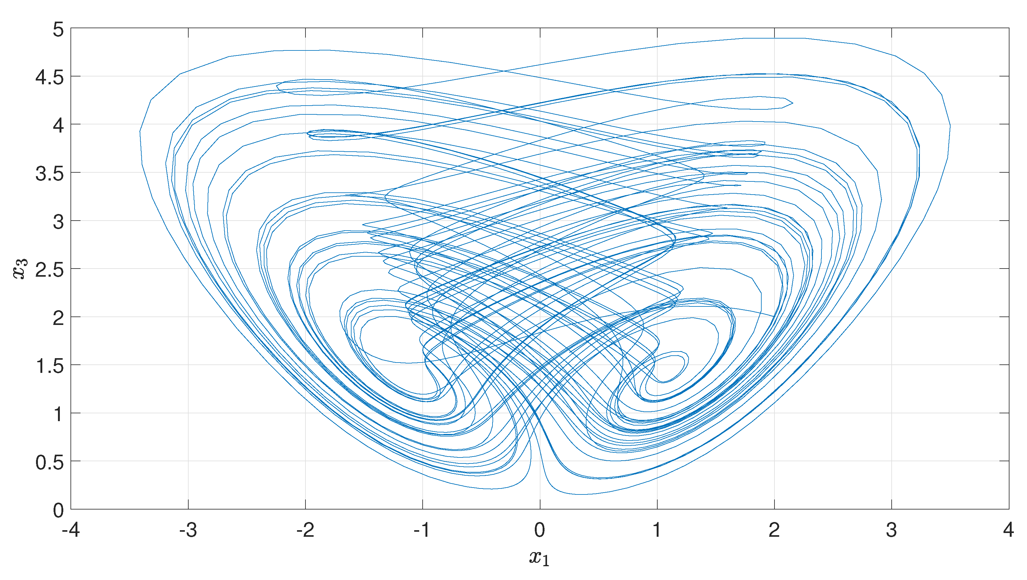
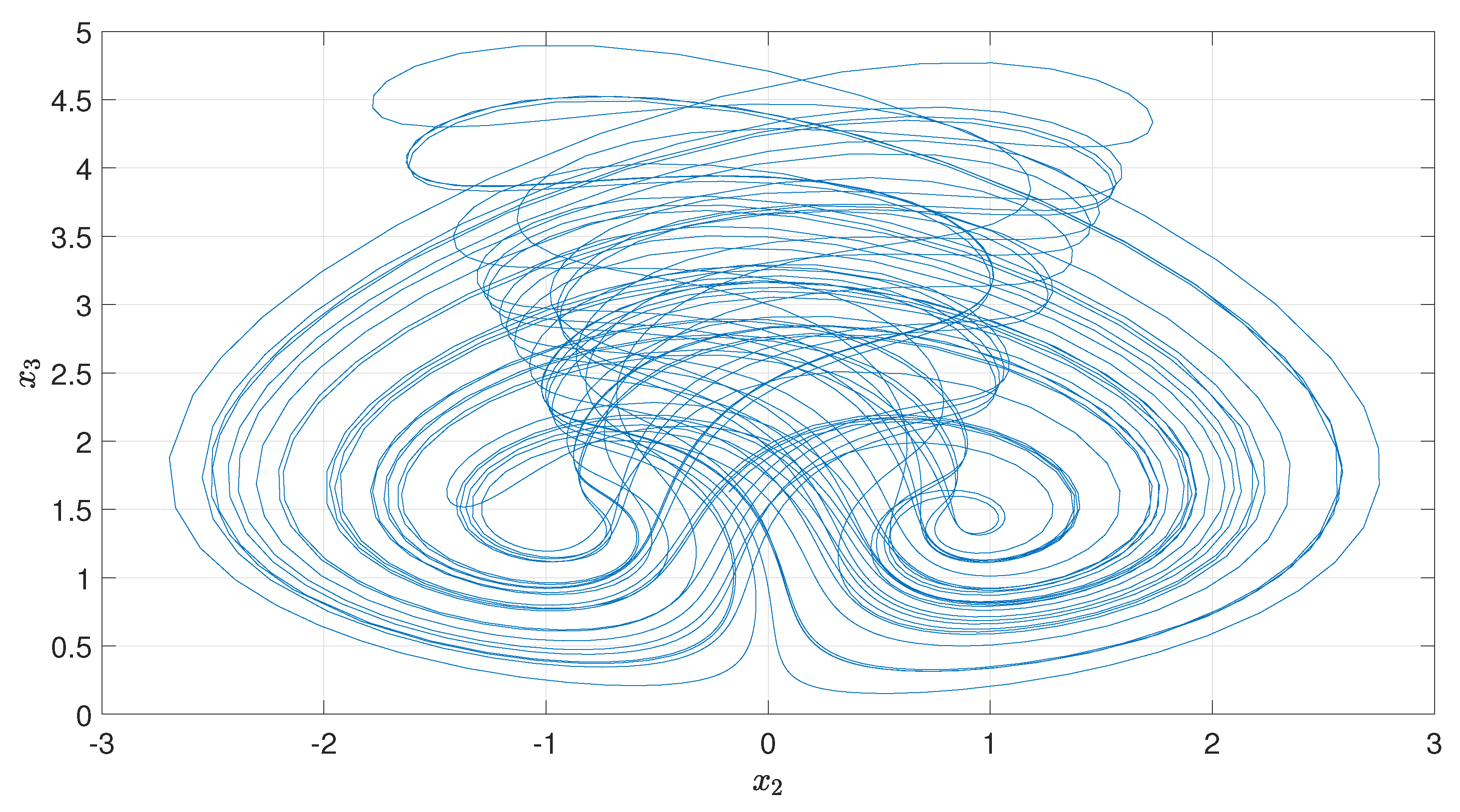
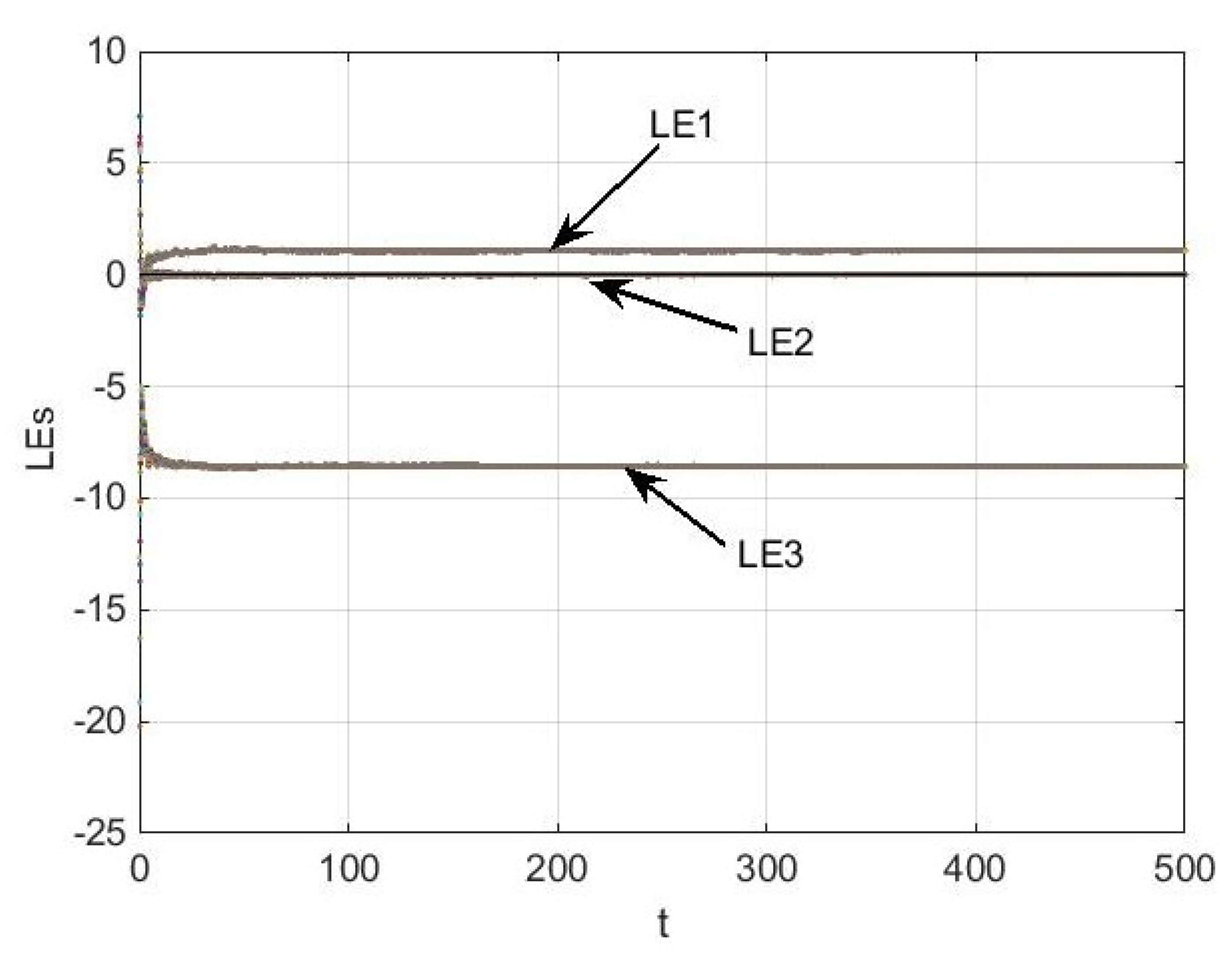
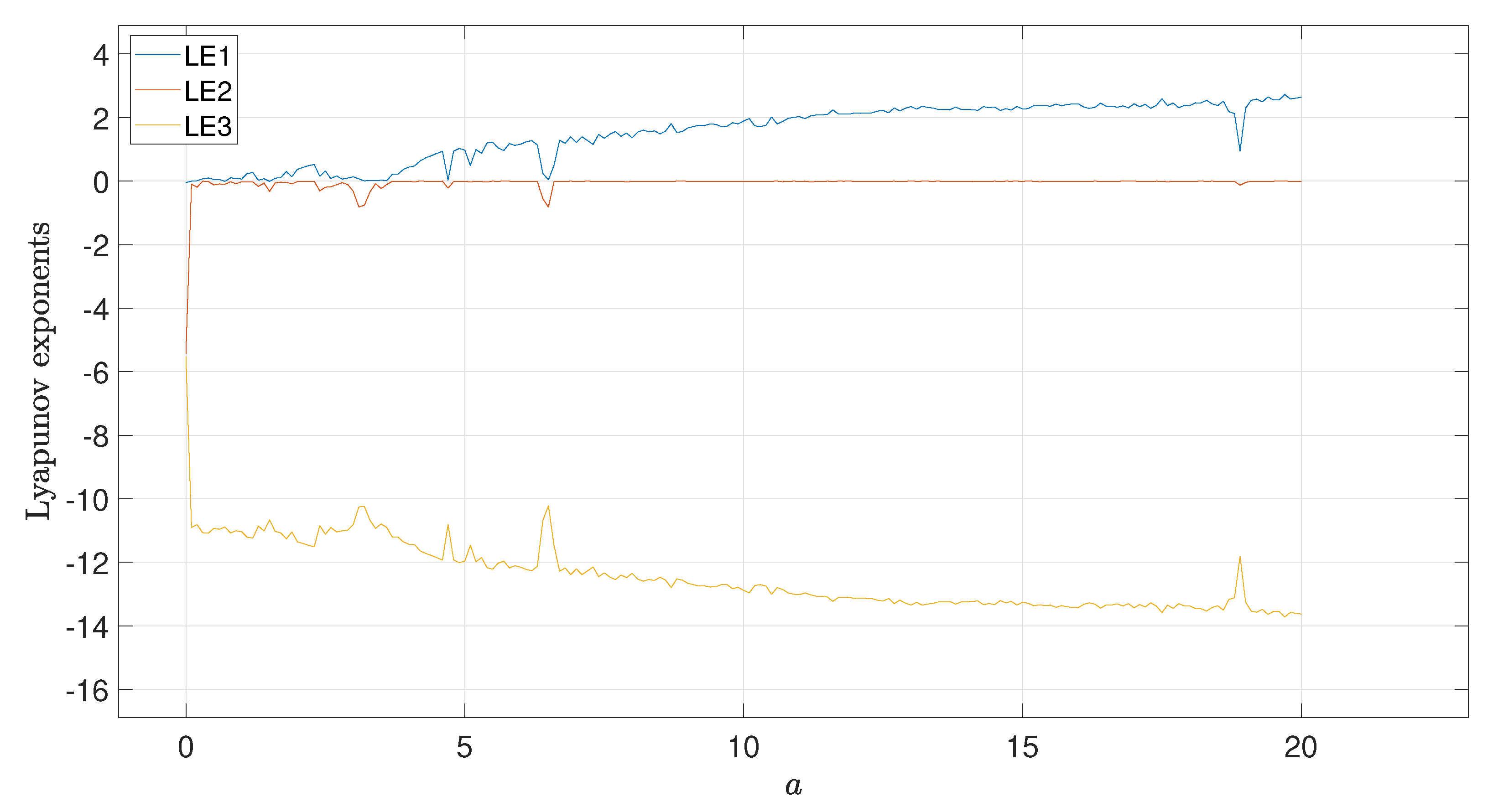
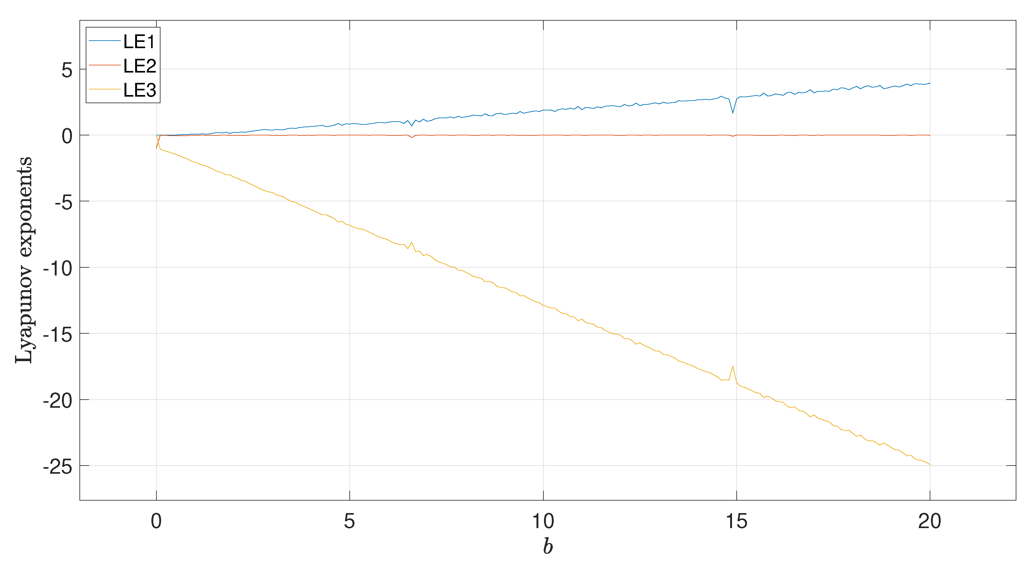
2.4. Lyapunov Exponents and Kaplan–York Dimension

Numerically, the chaotic system’s Lyapunov exponents for specific parameter values are obtained as:

$$LE1=1.0767,LE2=-0.0022\mathrm{and}\mathit{LE}3=-8.5677$$

Thus, the positive Lyaponuv exponent within the system shows that the system is chaotic.

Chaotic system’s Kaplan–York dimension is obtained as:

$$D_{KY}=j+\frac{1}{|{\lambda }_{j+1}|}\sum _{i=1}^j{\lambda }_i=2+\frac{{\lambda }_1+{\lambda }_2}{|{\lambda }_3|}=2+\frac{1.0767-0.0022}{|-8.5677|}=2.1254$$

Thus, the Lyapunov dimension is fractal dimension, depicting a chaotic system. Figure 3 illustrates Lyapunov exponent’s dynamics, which ensures the system’s chaos behavior. Moreover we have studied the spectrum of Lyapunov exponents for a and b as we can see in Figure 4 and Figure 5 respectively one exponent is bigger than zero, another is close to zero, and the third is smaller than zero.

3. Electronic Circuit and Signal Flow Graph

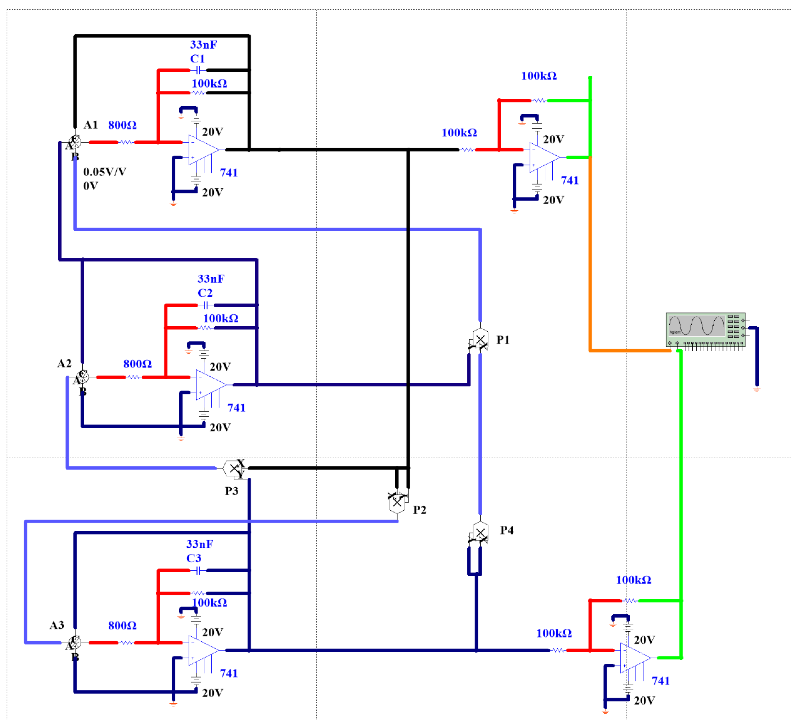
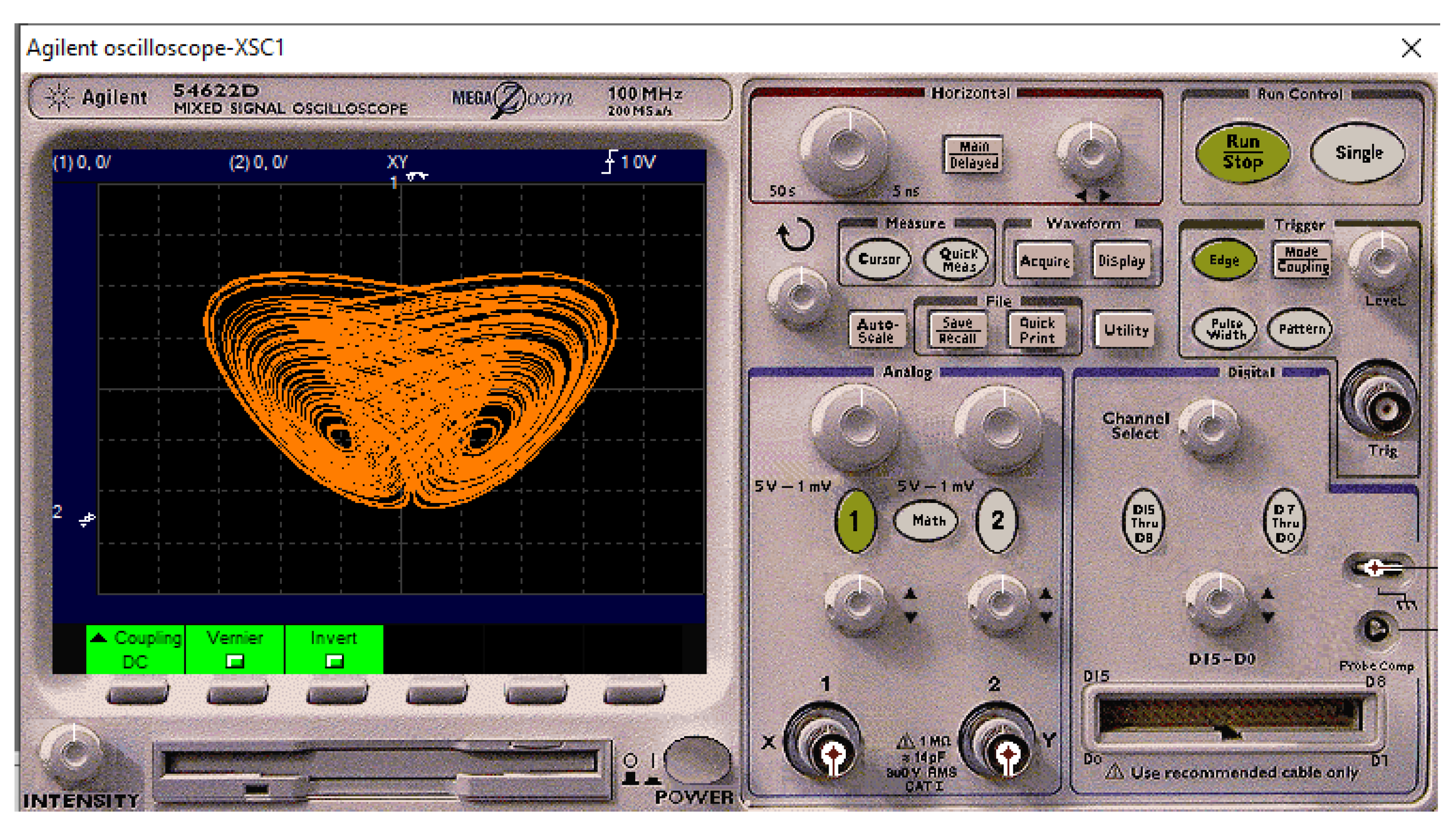
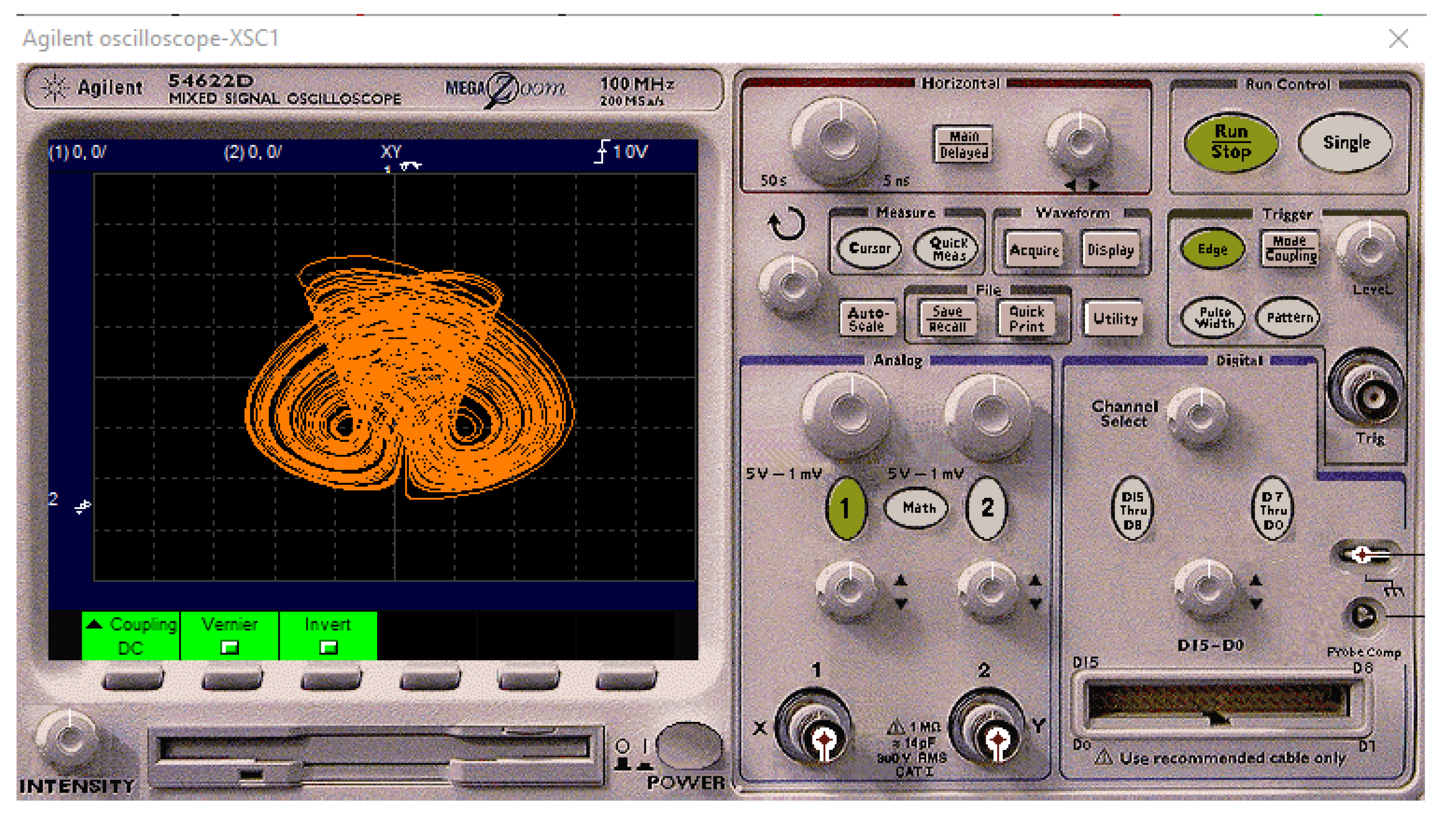
3.1. Electronic Circuit Implementation for System Realization

Chaotic systems are very important and used in several real applications in physics, nature, and secure communications. Consequently realizable chaotic models are very useful in this direction. It is very good result to build up an electronic circuit to realize a chaotic model and convert it from pure mathematics point of view to real object which mean its applicability. In this section, the proposed 3D chaotic model (1) is considered. The electronic circuit shown in Figure 6 was designed using the NI Multisim 14.0 package, where A1, A2, A3 are three summers, each with three inputs and a single output; P1, P2, P3, P4 are AD633 voltage multipliers, each with two inputs and a single output. All of the inputs and outputs are adjusted with identity gain. The three voltage integrators with outputs equivalent to the system states $x_1$ to $x_3$ are replicated with the help of three LM741 operational amplifiers. Moreover, two LM741 operational amplifiers help in generating two voltage inverters. Figure 6 presents the designed values of capacitors and resistors.

Table 1. The voltage summing devices used.

Summer Symbol	A	B	C	O
A1	−10	−1	10	0.05
A2	−3	3	−5	0.05
A3	3	0	2.5	0.05

shows the input/output gain’s used in the voltage summers. Figure 7 shows the $x_1$–$x_3$ phase plane from the real electronic circuit. Figure 8 shows the $x_2$–$x_3$ phase plane in the real electronic circuit.

The electronic circuit of our system show that our new system is applicable. The solutions of our system can use as signals in some application such as secure communication.

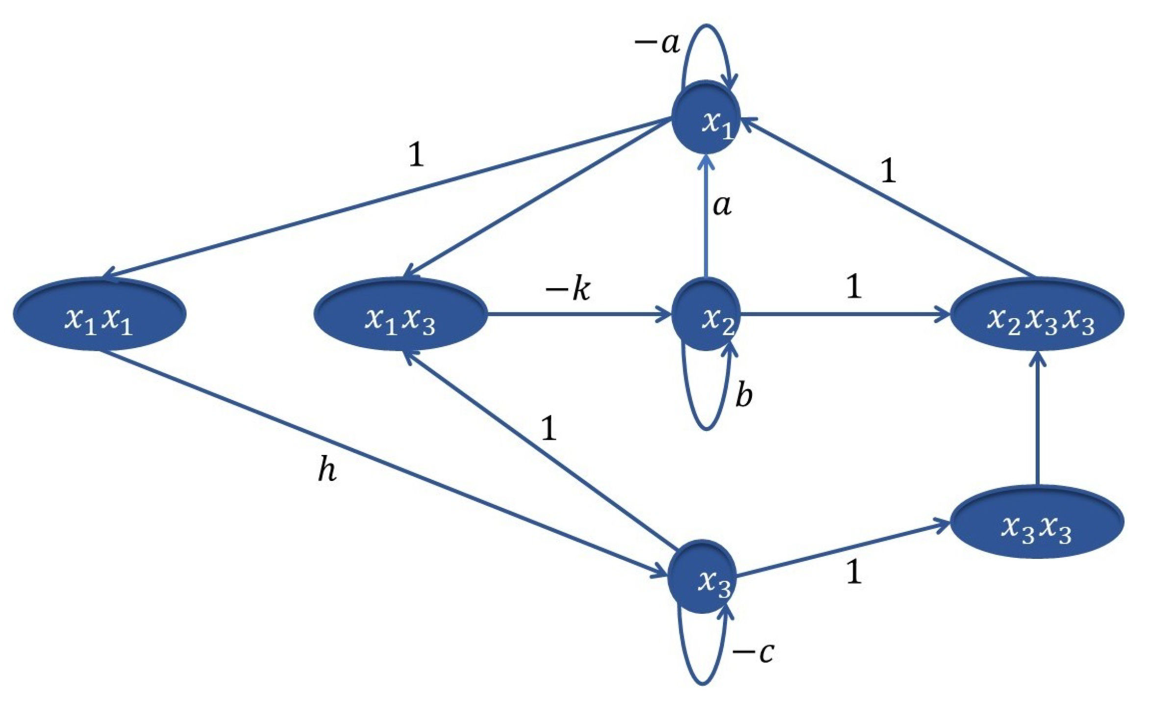
3.2. System’s Signal Flow Graph

A graphical tool for examining the relationships between system states is the signal flow graph. Signal flow graphs are highly useful for exploring the relationships between nonlinear dynamical systems, allowing for the nationalist and discovery of novel aspects of the nonlinear dynamical system under investigation. As they may be used to map the signals between the variables of the system, signal flow graphs are also helpful in the design and building of electrical circuits for dynamical nonlinear systems.

The interactions between the system states are displayed using some concepts of graph theory. Firstly, we construct a signal flow graph for the studied system and compute its energy from graph point of view. From the system (1), the model has three pure states $x_1$, $x_2$ and $x_3$ along with four hybrid states $x_1^2$, $x_2{x}_3^2$, $x_3^2$ and $x_1{x}_3$. Figure 9 shows the system signal flow graph D.

The Hermitian matrix of a digraph D may be defined as:

$$H_{uv}\left(D\right)=\left\{\begin{array}{c}1,\mathrm{if} (u,v)\mathrm{and} (v,u)\mathrm{are}\mathrm{edges}\mathrm{in}D;\hfill \\ \mathrm{i},\mathrm{if} (u,v)\mathrm{is}\mathrm{an}\mathrm{edge}\mathrm{in}D\mathrm{but} (v,u)\mathrm{is}\mathrm{not};\hfill \\ -\mathrm{i},\mathrm{if} (v,u)\mathrm{is}\mathrm{an}\mathrm{edge}\mathrm{in}D\mathrm{but} (u,v)\mathrm{is}\mathrm{not};\hfill \\ 0,\mathrm{otherwise}.\hfill \end{array}\right.$$

Then graph D has the following Hermitian matrix

$$H\left(D\right)=\begin{array}{c}{x}_1\\ x_2\\ x_3\\ x_1^2\\ x_3^2\\ x_1{x}_3\\ x_2{x}_3^2\end{array}\times \left[\begin{array}{ccccccc}1& -i& 0& i& 0& i& -i\\ i& 1& 0& 0& 0& -i& i\\ 0& 0& 1& -i& i& i& 0\\ -i& 0& i& 0& 0& 0& 0\\ 0& 0& -i& 0& 0& i& 0\\ -i& i& -i& 0& -i& 0& 0\\ i& -i& 0& 0& 0& 0& 0\end{array}\right]$$

.

The eigenvalues of $H\left(D\right)$ are: −2.0852, −1.4156, −0.3598, 0.3996, 0.9446, 2.4041, 3.1124. The definition of Hermitian energy is given as $EH\left(D\right)={\sum }_{i=1}^7=\left|{\mu }_i\right|=10.7213$, where 7 is the order of D and $\mu$ are Hermitian matrix’s eigenvalues. This energy value is new and can be used for comparison purposes.

4. Chaotic Behavior of System-Control

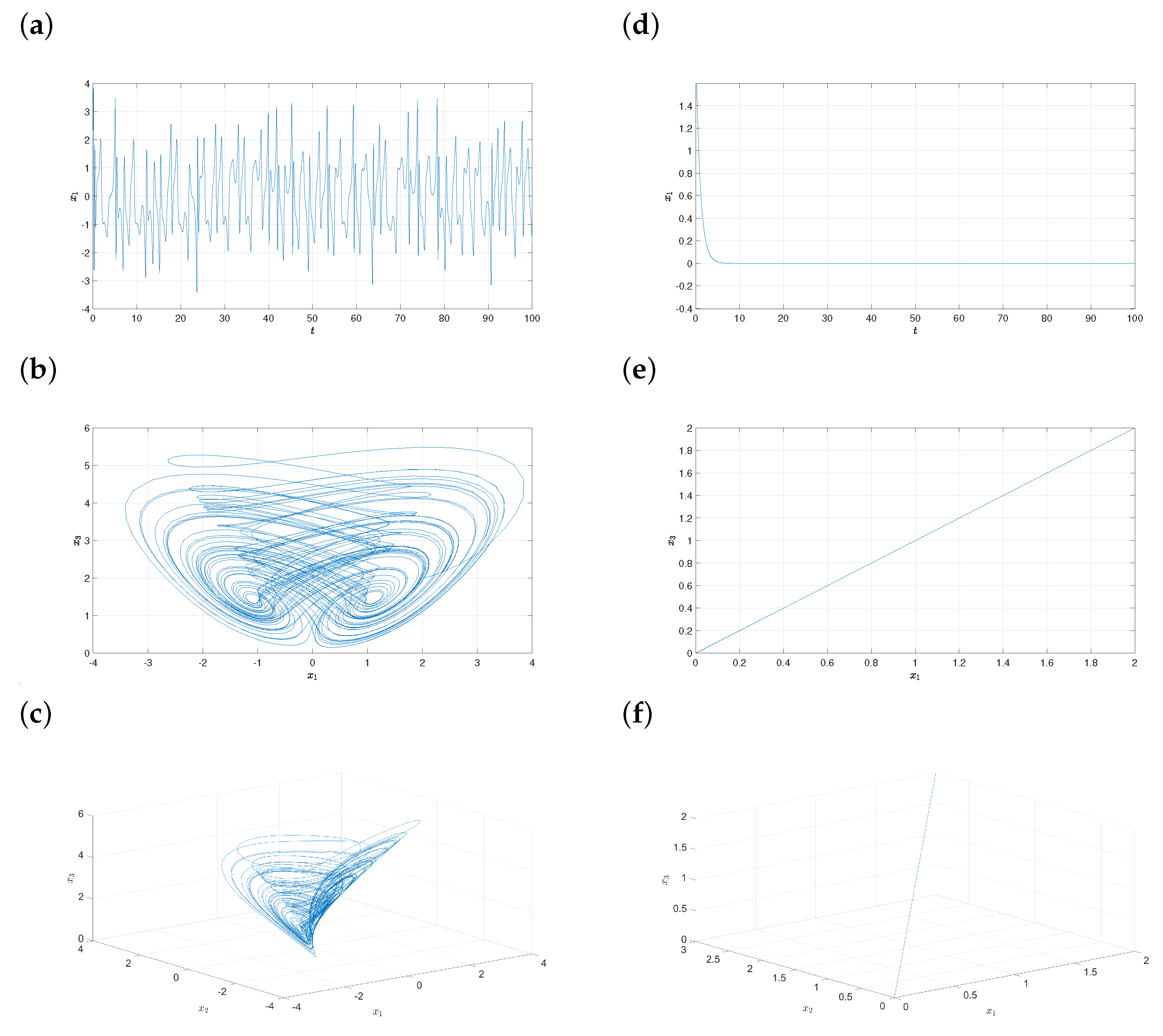
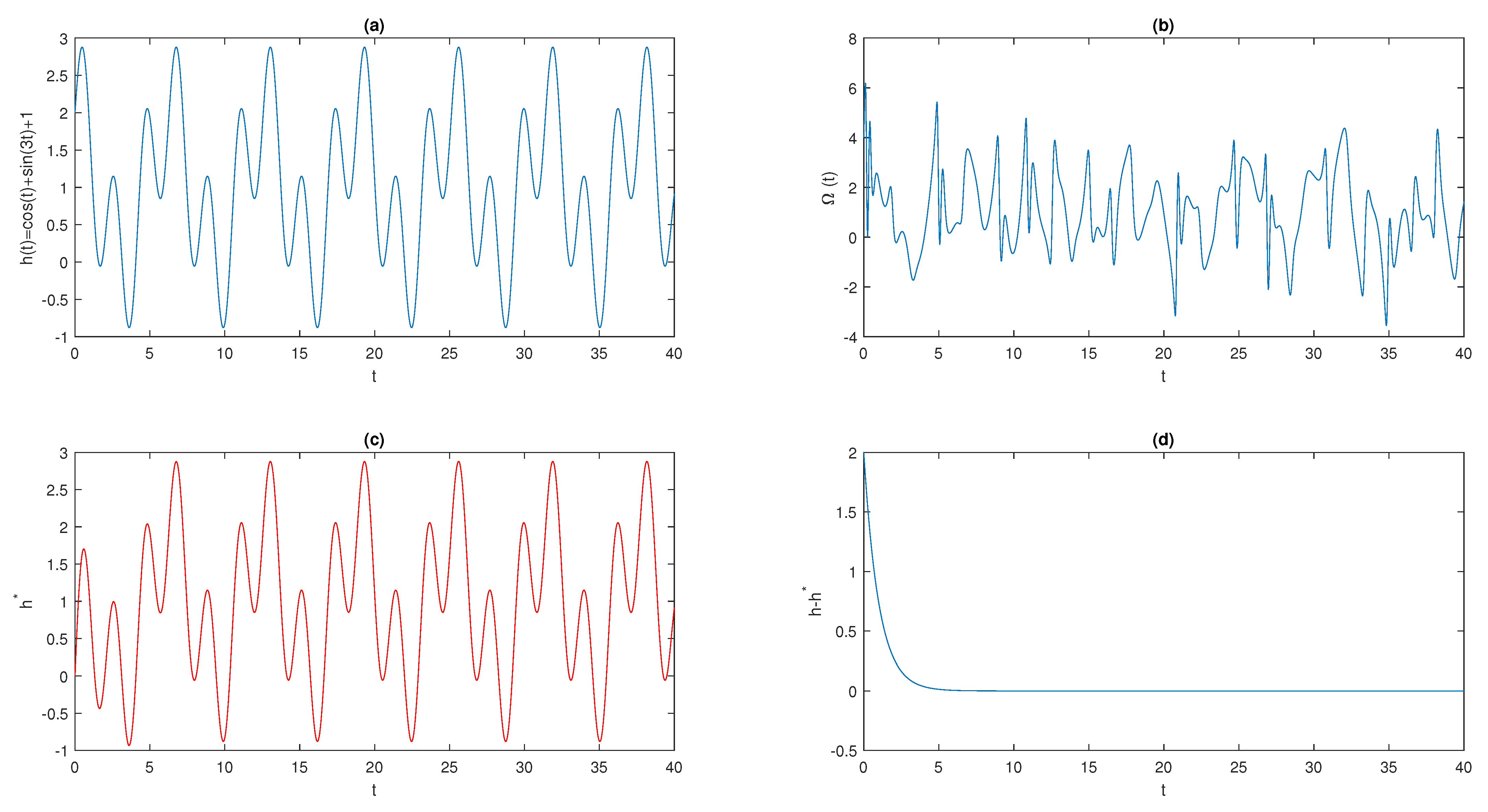
4.1. Analytical Solution

The term “chaos control for chaotic solutions” refers to the development of a controller capable of alleviating or reducing the chaotic behaviour of a nonlinear system. In this section, the Lyapunov stability theorem is utilized for suppressing the chaotic response to unstable trivial fixed point $E_0$.

Controlled new system’s equations are provided by:

$$\left\{\begin{array}{c}{x}_1^{\prime }=a(x_2-x_1)+x_2{x}_3^2+u_1,\hfill \\ x_2^{\prime }=b{x}_2-k{x}_1{x}_3+u_2,\hfill \\ x_3^{\prime }=h{x}_1^2-c{x}_3+u_3,\hfill \end{array}\right.$$

(3)

where $u_1,u_2$ and $u_3$ are controller functions to design. These controllers will be constructed appropriately for pushing the system’s trajectory towards unsteady trivial point $E_0$ of the uncontrolled system. The following Lyapunov function is chosen such that:

$$V\left(t\right)=\frac{1}{2}\sum _{i=1}^3{x}_i^2$$

time derivative of $V\left(t\right)$ is:

$$\begin{array}{cc}\hfill V^{\prime }\left(t\right)& =\sum _{i=1}^3{x}_i{x}_i^{\prime }=x_1{x}_1^{\prime }+x_2{x}_2^{\prime }+x_3{x}_3^{\prime }\hfill \\ & =x_1[a(x_2-x_1)+x_2{x}_3^2+u_1]+x_2[b{x}_2-k{x}_1{x}_3+u_2]+x_3[h{x}_1^2-c{x}_3+u_3]\hfill \end{array}$$

considring the controllers $u_i,i=1,2,3$ as below:

$$\left\{\begin{array}{c}{u}_1=-x_1-a(x_2-x_1)+x_2{x}_3^2,\hfill \\ u_2=-x_2-b{x}_2+k{x}_1{x}_3,\hfill \\ u_3=-x_3-h{x}_1^2+c{x}_3,\hfill \end{array}\right.$$

(4)

the Lyapunov function’s time derivative yields:

$$V^{\prime }\left(t\right)=-x_1^2-x_2^2-x_3^2<0.$$

Therefore, controlled system and unstable equilibrium point $E_0$ may converge asymptotically, such that $u_i=0,i=1,2,3$ as $t\to \infty$.

4.2. Numerical Simulation

The computer simulation is performed to evaluate the recommended controller’s performance. The system (3) without the controller was solved for the cases $a=10,$$b=5, c=2.5, h=3$ and $k=3$, where system’s chaotic attractors occur, as illustrated in Figure 10a–c. Figure 10a depicts the state variable $x_1$ of the system (1) (before control), and additional state variables. Whereas, Figure 10b,c shows the chaotic attractors of (1) plotted in $(x_1,x_2)$ plane and $(x_1,x_2,x_3)$ space, respectively. System (3) with the controllers (4) are numerically solved (after control), with the with similar parameters (Figure 10a–c). Chaotic solutions are translated to trivial fixed point, as predicted from the preceding analytical arguments. Figure 10d–f illustrates that control is attained within a short time period, which demonstrates effective outcomes. All numerical simulation results are done by using MATLAB Program with (ode45) code.

5. Complete Synchronization of Identical Chaotic System

5.1. Analytical Solution

In this section, a complete controller is constructed for the identical chaotic system synchronization. The complete controller design is conducted with the help of Lyapunov stability theory. The chaotic system is considered as a master system such that:

$$\left\{\begin{array}{c}{x}_1^{\prime }=a(x_2-x_1)+x_2{x}_3^2,\hfill \\ x_2^{\prime }=b{x}_2-k{x}_1{x}_3,\hfill \\ x_3^{\prime }=h{x}_1^2-c{x}_3,\hfill \end{array}\right.$$

(5)

where $x_1,x_2$ and $x_3$ are state variable and $a,b,c,h$ and k are parameters as mentioned in Section 2. As the slave system, chaotic system is considered:

$$\left\{\begin{array}{c}{y}_1^{\prime }=a(y_2-y_1)+y_2{y}_3^2+u_1,\hfill \\ y_2^{\prime }=b{y}_2-k{y}_1{y}_3+u_2,\hfill \\ y_3^{\prime }=h{y}_1^2-c{y}_3+u_3,\hfill \end{array}\right.$$

(6)

where $y_1,y_2$ and $y_3$ are state variable and $u_1,u_2$ and $u_3$ are controller functions.

The complete synchronization error between the slave and master system is explained as:

$$\left\{\begin{array}{c}{e}_1=y_1-x_1,\hfill \\ e_2=y_2-x_2,\hfill \\ e_3=y_3-x_3.\hfill \end{array}\right.$$

(7)

The error dynamics is easily calculated as:

$$\left\{\begin{array}{c}{e}_1^{\prime }=a(y_2-y_1)+y_2{y}_3^2-a(x_2-x_1)-x_2{x}_3^2+u_1,\hfill \\ e_2^{\prime }=b{y}_2-k{y}_1{y}_3-b{x}_2+k{x}_1{x}_3+u_2,\hfill \\ e_3^{\prime }=h{y}_1^2-c{y}_3-h{x}_1^2+c{x}_3+u_3.\hfill \end{array}\right.$$

(8)

The complete controller is defined by:

$$\left\{\begin{array}{c}{u}_1=-a{y}_2-y_2{y}_3^2+a{x}_2+x_2{x}_3^2,\hfill \\ u_2=-2b{y}_2+k{y}_1{y}_3+2b{x}_2-k{x}_1{x}_3,\hfill \\ u_3=-h{y}_1^2+h{x}_1^2.\hfill \end{array}\right.$$

(9)

Consider Lyapunov function explained by:

$$V=\frac{1}{2}(e_1^2+e_2^2+e_3^2),$$

which is definite and positive on $R^3$. The differentiation helps to attain V:

$$V^{\prime }=e_1{e}_1^{\prime }+e_2{e}_2^{\prime }+e_3{e}_3^{\prime }=-a{e}_1^2-b{e}_2^2-c{e}_3^2.$$

Since $V^{\prime }$ is negative definite on $R^3$, this demonstrates that the slave system synchronises with the master system in the sense of complete synchronization by the controller (9).

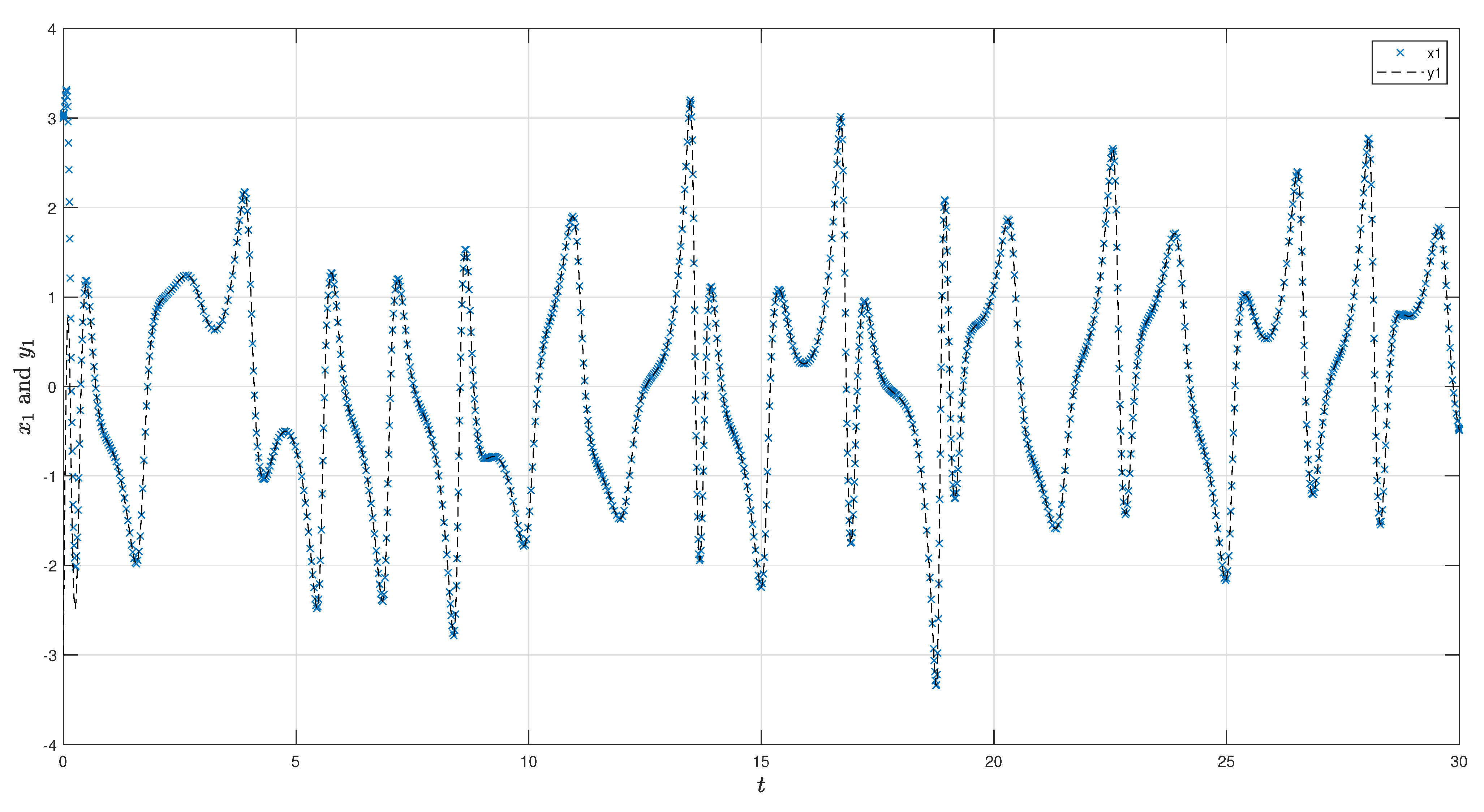
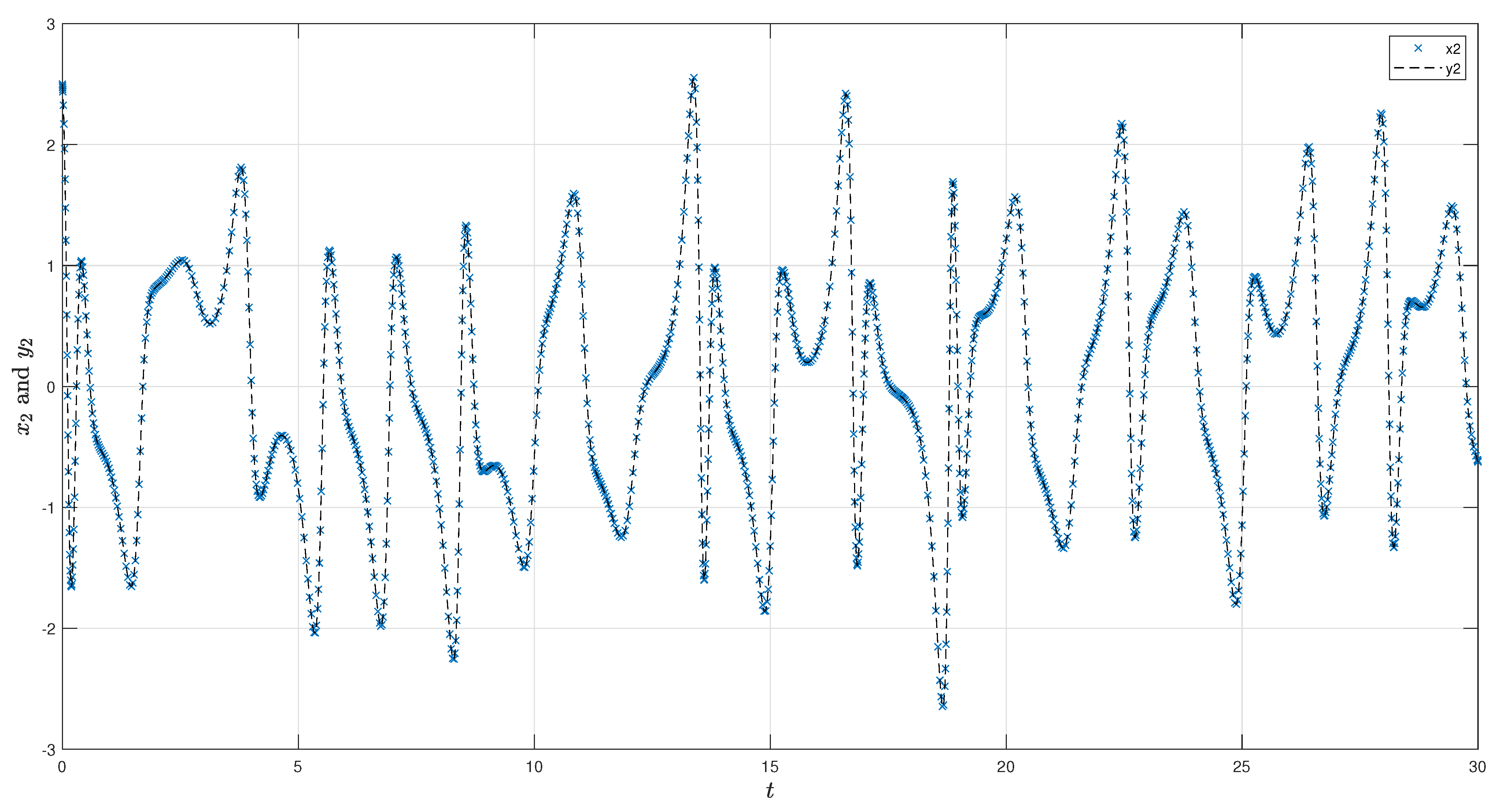
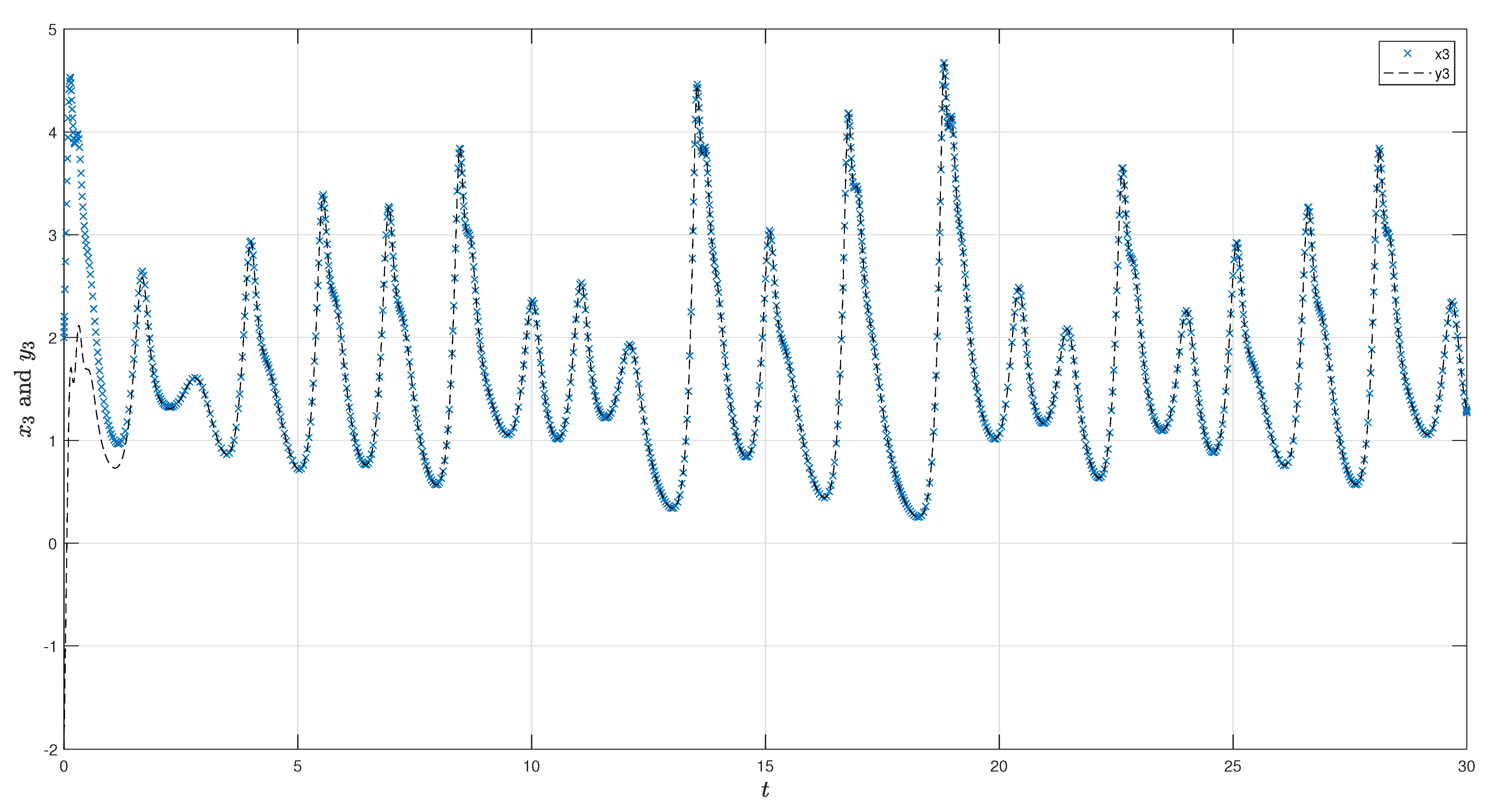
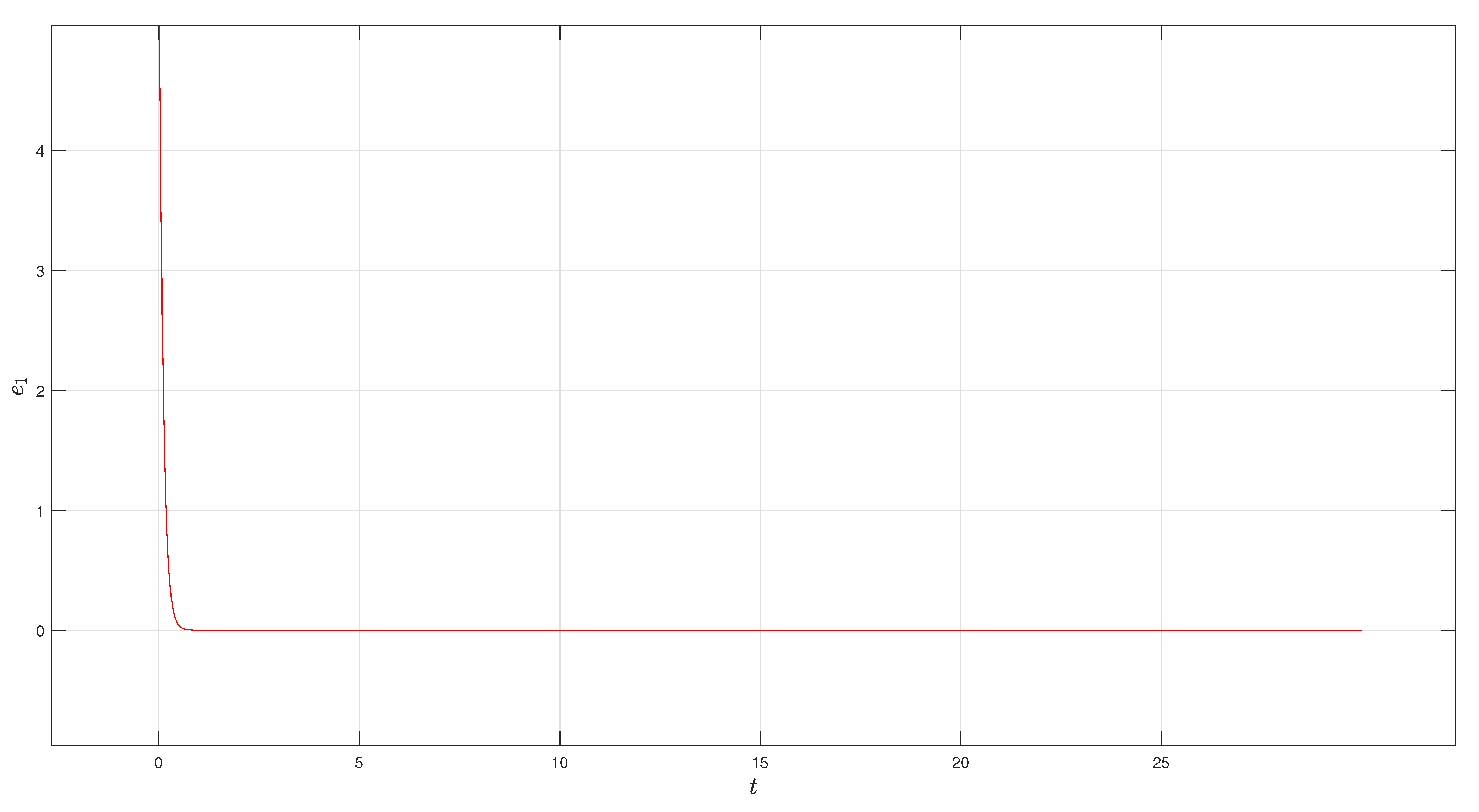
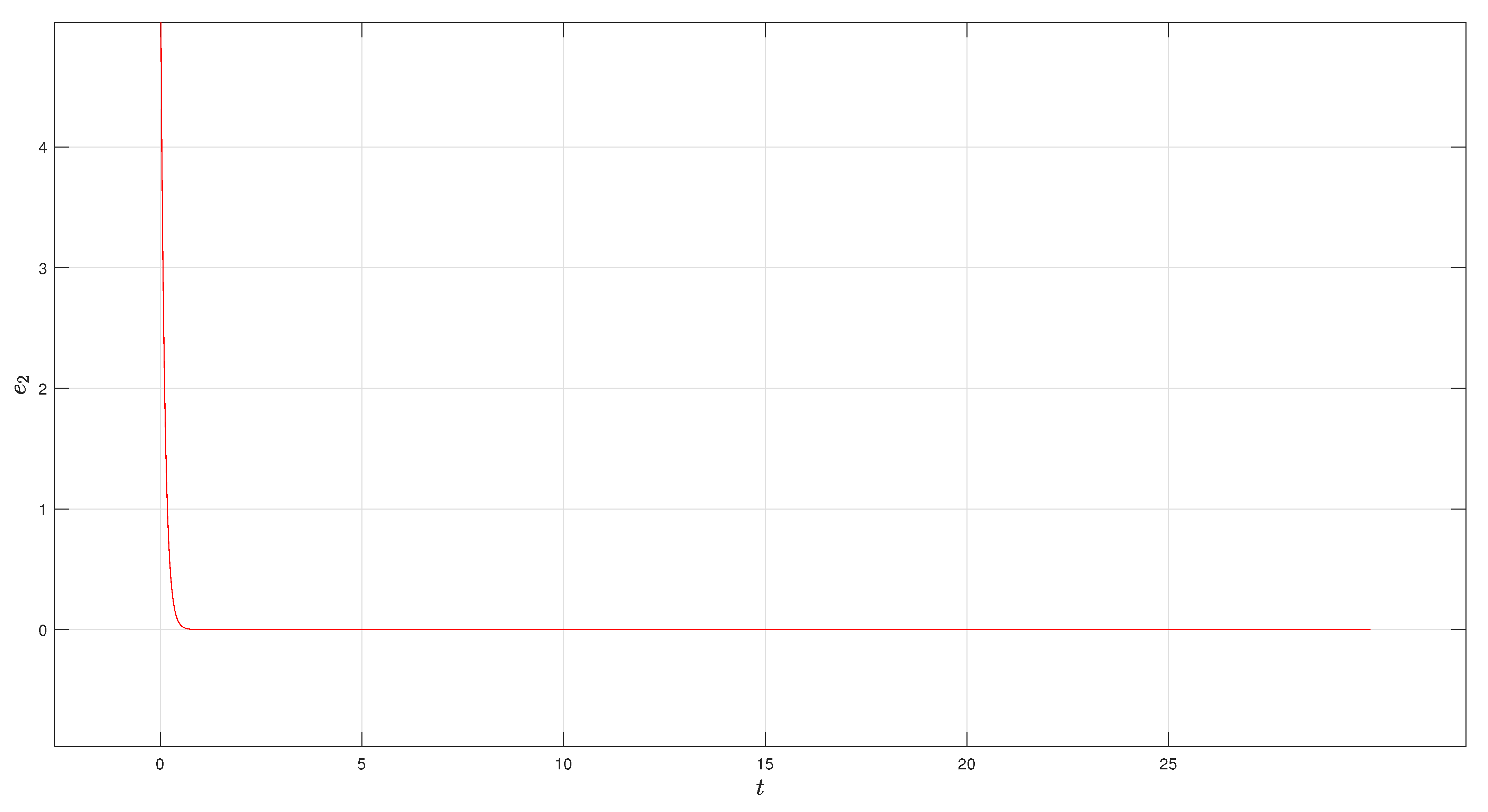
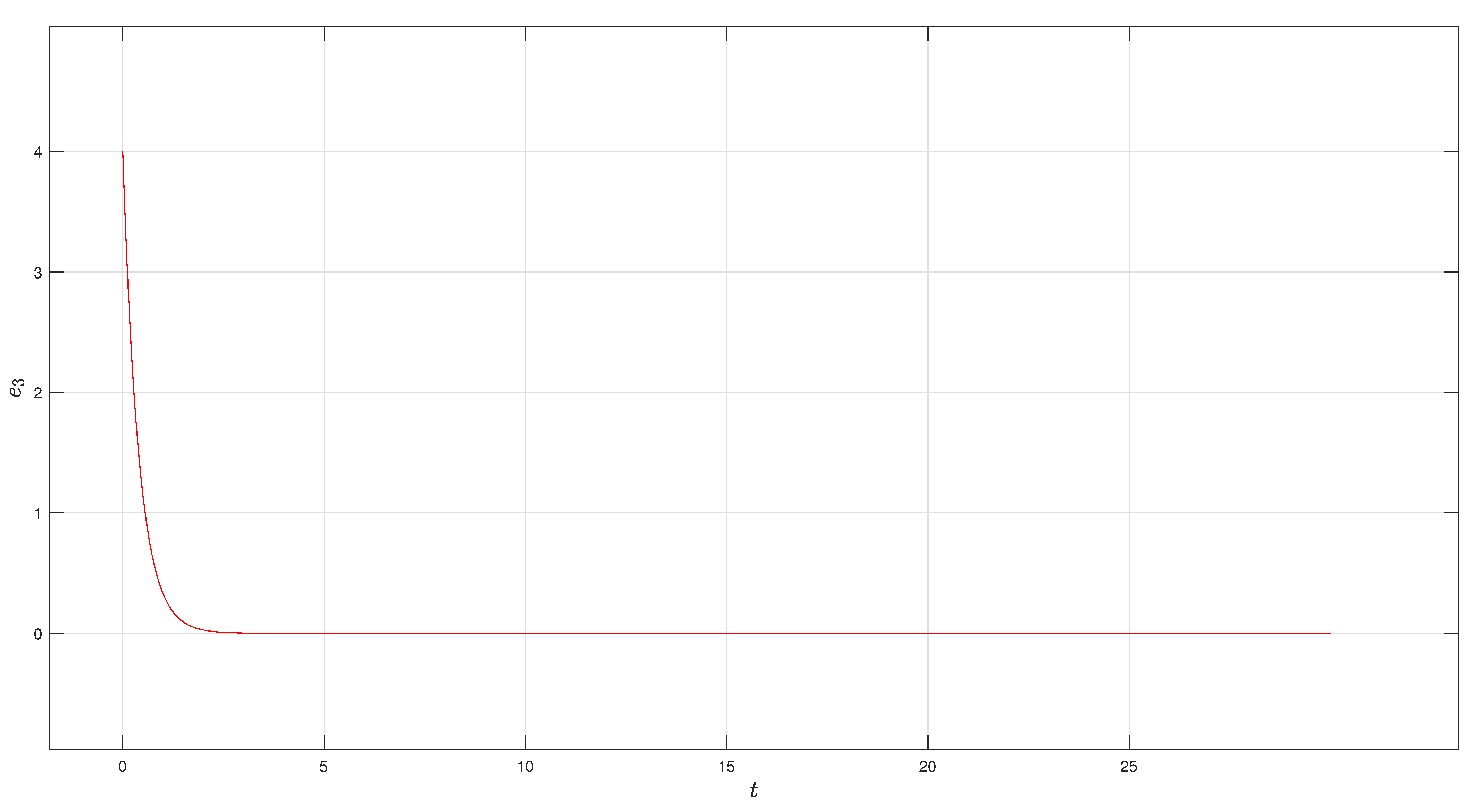
5.2. Numerical Simulation

The numerical results are made by using MATLAB program with (ode45) code. The simulation results of the chaotic systems (5) and (6) were expected to validate the efficacy of the proposed results. The systems (5) and (6) with the controller (9), for which system’s existing chaotic attractors were solved numerically. The master (5) and slave (6) system’s initial conditions are selected such that $(x_1\left(0\right),x_2\left(0\right),x_3\left(0\right))=(3,2.5,2)$ and $(y_1\left(0\right),y_2\left(0\right),y_3\left(0\right))=(-3,-2.5,-2)$. Figure 11, Figure 12 and Figure 13 illustrate the variable’s states via synchronizing manner between slave and master systems based on the study’s model. The solutions of (5) and (6) are displayed for various beginning circumstances to demonstrate chaotic synchronization after a short time period t. The state variable’s curves $x_i$, for $i=1,2,3$ are denoted using black dashed lines, and state variable’s curves $y_i$, for $i=1,2,3$ are denoted by blue stars lines. The synchronization error are plotted in Figure 14, Figure 15 and Figure 16, and it’s clear from these figures the synchronization is achieved after small time. This means our proposed controllers are very effect.

5.3. An Application in Secure Communications

The goal of chaotic communications, an implementation of the chaos hypothesis, is to ensure the safety of data transmissions made possible by technological advances in media communications. To understand what we mean by “secure communications”, one must realize that the information contained in the transmitted message is inaccessible to any third parties that could try to snoop on the conversation. Chaotic frameworks’ complicated dynamic characteristics are crucial to the security of chaotic communication. Several features of chaotic dynamics are exploited as encoding mechanisms, including complicated behavior, clamor like aspects, and dispersed range.

Chaotic communications based on past qualities require two chaotic oscillators, one to serve as a transmitter and one as a receiver. A message is hidden in the noise of a chaotic signal and transmitted from the transmitter. The chaotic signal is also known as the chaotic bearer because of its role in transmitting information. For purposes of neural cryptography, synchronizing these oscillators is analogous to synchronizing asynchronous neural cryptography [34,35,36].

The outcomes of the new system’s chaotic synchronization use a simple approach to produce application in a secure communications. The master system (5) was considered as the transmitter system, the reception system denoted the slave system (5). The transmitter system’s encryption of message signal $h\left(t\right)$ and chaotic signals are expressed by an invertible nonlinear function, with addition of signal $h\left(t\right)$ to one (or more) of the three variables $x_{1m},x_{2m},x_{3m}$ (where $x_{1m},x_{2m},x_{3m}$ are the state variable of the master system) in the later step. For example, the combined signal is $\Omega =h\left(t\right)+x_{1m}$ by adding it into the variable $x_{1m}$. Then, the combination of chaotic signals of the transmitter system are transmitted towards receiver side. So, the chaos synchronization between two similar chaotic complexes (5), (6) systems is likely to be attainted after some time $t_s$. The states of $x_m$ will approach to $x_s$. At a certain time $t_c$ i.e., time greater than $x_s$ ($x_s$ is the beginning time of the synchronization process), the receiver starts to recover $\Omega \left(t\right)$ via a simple transformation $h^{*}=\Omega \left(t\right)-x_{1s}$.

In the following numerical simulations, the system characteristics and transmitter and reception systems’ initial circumstances are assumed to similar as stated in Section 2. Figure 17 depicts a numerical simulation of using chaotic synchronization in secure communication. The message $h\left(t\right)$ and the transmitted signal $\Omega \left(t\right)$ are illustrated in Figure 17a,b respectively. Figure 17c shows the recovered message $h^{*}\left(t\right)$. The error between the original and recovered message is illustrated in Figure 17d.

6. Conclusions

The present study has proposed new chaotic system that includes its dynamics, electronic circuit, signal flow graph, chaos control, and chaos synchronization. Lyapunov stability theorem is used for designing the control laws that is likely to help in achieve equilibrium of the chaotic system. The complete synchronization of the proposed chaotic system is also studied and based on the Lyapunov stability theory (see Figure 11, Figure 12 and Figure 13). The synchronization errors are shown in Figure 14, Figure 15 and Figure 16. From these figures it’s clear the synchronization is achieved. The chaos synchronization develops a simple application within the secure communications. The numarical results of secure communication are illustrated in Figure 17.

The numerical simulations verify all the theoretical results for further demonstrating effectiveness of proposed schemes. The verification of all the theoretical results is done by numerical simulations that further explains the proposed scheme’s effectiveness.

References

1. Qi, G.; Chen, G.; Du, S.; Chen, Z.; Yuan, Z. Analysis of a new chaotic system. Phys. A Stat. Mech. Appl. 2005, 352, 295–308. [Google Scholar] [CrossRef]
2. Qi, G.; Chen, Z.; Yuan, Z. Model-free control of affine chaotic systems. Phys. Lett. A 2005, 344, 189–202. [Google Scholar] [CrossRef]
3. Nana Nbendjo, B.R.; Woafo, P. Active control with delay of horseshoes chaos using piezoelectric absorber on a buckled beam under parametric excitation. Chaos Solitons Fractals 2007, 32, 73–79. [Google Scholar] [CrossRef]
4. Park, J.H. Chaos synchronization between two different chaotic dynamical systems. Chaos Solitons Fractals 2006, 27, 549–554. [Google Scholar] [CrossRef]
5. Wu, C.; Fang, T.; Rong, H. Chaos synchronization of two stochastic duffing oscillators by feedback control. Chaos Solitons Fractals 2007, 32, 1201–1207. [Google Scholar] [CrossRef]
6. Moon, F.C. Chaotic and Fractal Dynamics; Wiley: New York, NY, USA, 1992. [Google Scholar]
7. Khalil, H.K. Nonlinear System; Macmillan Publishing Company: New York, NY, USA, 1992. [Google Scholar]
8. Mahmoud, E.E.; Mahmoud, G.M. Some Chaotic Complex Nonlinear Systems; Lambert Academic Publishing: Saarbrücken, Germany, 2010. [Google Scholar]
9. Mahmoud, E.E.; Mahmoud, G.M. Chaotic and Hyperchaotic Nonlinear Systems; Lambert Academic Publishing: Saarbrücken, Germany, 2011. [Google Scholar]
10. Eppinger, D.S.; Browning, R.T. Design Structure Matrix Methods and Applications; MIT Press: Cambridge, MA, USA, 2012. [Google Scholar]
11. Mezit, I.; Vladimir, A.; Fonoberov, M.F.; Sahai, T. Spectral complexity of directed graphs and application to structural decomposition. Complexity 2019, 2019, 18. [Google Scholar]
12. Ma, C.; Mou, J.; Xiong, L.; Banerjee, S.; Liu, T.; Han, X. Dynamical analysis of a new chaotic system: Asymmetric multistability, offset boosting control and circuit realization. Nonlinear Dyn. 2021, 103, 2867–2880. [Google Scholar] [CrossRef]
13. Vaidyanathan, S.; Pehlivan, İ.; Dolvis, L.G.; Jacques, K.; Alcin, M.; Tuna, M.; Koyuncu, I. A novel ANN-based four-dimensional two-disk hyperchaotic dynamical system, bifurcation analysis, circuit realisation and FPGA-based TRNG implementation. Int. J. Comput. Appl. Technol. 2020, 62, 20–35. [Google Scholar] [CrossRef]
14. Takhi, H.; Kemih, K.; Moysis, L.; Volos, C. Passivity based sliding mode control and synchronization of a perturbed uncertain unified chaotic system. Math. Comput. Simul. 2021, 181, 150–169. [Google Scholar] [CrossRef]
15. Darbasi, S.; Mirzaei, M.J.; Abazari, A.M.; Rezazadeh, G. Adaptive under-actuated control for capacitive micro-machined ultrasonic transducer based on an accurate nonlinear modeling. Nonlinear Dyn. 2022, 108, 2309–2322. [Google Scholar] [CrossRef]
16. Tian, H.; Wang, Z.; Zhang, P.; Chen, M.; Wang, Y. Dynamic analysis and robust control of a chaotic system with hidden attractor. Complexity 2021, 2021, 1–11. [Google Scholar] [CrossRef]
17. Tong, Y.; Cao, Z.; Yang, H.; Li, C.; Yu, W. Design of a five-dimensional fractional-order chaotic system and its sliding mode control. Indian J. Phys. 2022, 96, 855–867. [Google Scholar] [CrossRef]
18. Tiwari, A.; Nathasarma, R.; Roy, B.K. A 3D chaotic system with dissipative and conservative behaviors and its control using two linear active controllers. In Proceedings of the 2022 4th International Conference on Energy, Power and Environment (ICEPE), Shillong, India, 29 April–1 May 2022; Volume 29, pp. 1–6. [Google Scholar]
19. Rybin, V.; Tutueva, A.; Karimov, T.; Kolev, G.; Butusov, D.; Rodionova, E. Optimizing the Synchronization Parameters in Adaptive Models of Rössler system. In Proceedings of the 2021 10th Mediterranean Conference on Embedded Computing (MECO), Budva, Montenegro, 7–10 June 2021; pp. 1–4. [Google Scholar] [CrossRef]
20. Rybin, V.; Kolev, G.; Kopets, E.; Dautov, A.; Karimov, A.; Karimov, T. Optimal Synchronization Parameters for Variable Symmetry Discrete Models of Chaotic Systems. In Proceedings of the 2022 11th Mediterranean Conference on Embedded Computing (MECO), Budva, Montenegro, 7–10 June 2022; pp. 1–5. [Google Scholar] [CrossRef]
21. Dana, S.K.; Roy, P.K.; Kurths, J. (Eds.) Complex Dynamics in Physiological Systems: From Heart to Brain; Springer Science & Business Media: New York, NY, USA, 2008. [Google Scholar]
22. Pecora, L.M.; Carroll, T.L. Synchronization in chaotic systems. Phys. Rev. Lett. 1990, 64, 821. [Google Scholar] [CrossRef] [PubMed]
23. Rosenblum, M.G.; Pikovsky, A.S.; Kurths, J. Phase synchronization of chaotic oscillators. Phys. Rev. Lett. 1996, 76, 1804. [Google Scholar] [CrossRef] [Green Version]
24. Rulkov, N.F.; Sushchik, M.M.; Tsimring, L.S.; Abarbanel, H.D. Generalized synchronization of chaos in directionally coupled chaotic systems. Phys. Rev. E 1995, 51, 980. [Google Scholar] [CrossRef]
25. Rosenblum, M.G.; Pikovsky, A.S.; Kurths, J. From phase to lag synchronization in coupled chaotic oscillators. Phys. Rev. Lett. 1997, 78, 4193. [Google Scholar] [CrossRef]
26. Boccaletti, S.; Valladares, D.L. Characterization of intermittent lag synchronization. Phys. Rev. E 2000, 62, 7497. [Google Scholar] [CrossRef] [PubMed] [Green Version]
27. Hramov, A.E.; Koronovskii, A.A. An approach to chaotic synchronization. Chaos Interdiscip. J. Nonlinear Sci. 2004, 14, 603–610. [Google Scholar] [CrossRef] [Green Version]
28. Hramov, A.E.; Koronovskii, A.A.; Moskalenko, O.I. Generalized synchronization onset. EPL (Europhys. Lett.) 2005, 72, 901. [Google Scholar] [CrossRef] [Green Version]
29. Mainieri, R.; Rehacek, J. Projective synchronization in three-dimensional chaotic systems. Phys. Rev. Lett. 1999, 82, 3042. [Google Scholar] [CrossRef]
30. Li, G.H. Generalized projective synchronization between Lorenz system and Chen’s system. Chaos Solitons Fractals 2007, 32, 1454–1458. [Google Scholar] [CrossRef]
31. Du, H.; Zeng, Q.; Wang, C. Function projective synchronization of different chaotic systems with uncertain parameters. Phys. Lett. A 2008, 372, 5402–5410. [Google Scholar] [CrossRef]
32. Sudheer, K.S.; Sabir, M. Adaptive function projective synchronization of two-cell Quantum-CNN chaotic oscillators with uncertain parameters. Phys. Lett. A 2009, 373, 1847–1851. [Google Scholar] [CrossRef]
33. Sudheer, K.S.; Sabir, M. Function projective synchronization in chaotic and hyperchaotic systems through open-plus-closed-loop coupling. Chaos Interdiscip. J. Nonlinear Sci. 2010, 20, 013115. [Google Scholar] [CrossRef] [PubMed]
34. Tutueva, A.; Moysis, L.; Rybin, V.; Zubarev, A.; Volos, C.; Butusov, D. Adaptive symmetry control in secure communication systems. Chaos Solitons Fractals 2022, 159, 112181. [Google Scholar] [CrossRef]
35. Rybin, V.; Butusov, D.; Rodionova, E.; Karimov, T.; Ostrovskii, V.; Tutueva, A. Discovering Chaos-Based Communications by Recurrence Quantification and Quantified Return Map Analyses. Int. J. Bifurc. Chaos 2022, 32, 2250136. [Google Scholar] [CrossRef]
36. Rybin, V.; Karimov, T.; Bayazitov, O.; Kvitko, D.; Babkin, I.; Shirnin, K.; Kolev, G.; Butusov, D. Prototyping the Symmetry-Based Chaotic Communication System Using Microcontroller Unit. Appl. Sci. 2023, 13, 936. [Google Scholar] [CrossRef]
Figure 1. x 1 x 3 Phase portrait of new chaotic system.
Fractalfract 07 00253 g001
Figure 2. x 2 x 3 Phase portrait of new chaotic system.
Fractalfract 07 00253 g002
Figure 3. Lyapunov exponents of model (1).
Fractalfract 07 00253 g003
Figure 4. Spectrum of Lyapunov exponents for variable a.
Fractalfract 07 00253 g004
Figure 5. Spectrum of Lyapunov exponents for variable b.
Fractalfract 07 00253 g005
Figure 6. Electronic circuit realization of the system (1).
Fractalfract 07 00253 g006
Figure 7. The x 1 x 3 phase plane from the real electronic circuit.
Fractalfract 07 00253 g007
Figure 8. The x 2 x 3 phase plane from the real electronic circuit.
Fractalfract 07 00253 g008
Figure 9. System signal flow directed graph D.
Fractalfract 07 00253 g009
Figure 10. Numerical solution of system (3): (ac) before control, and (df) after control.
Fractalfract 07 00253 g010
Figure 11. Synchronization of system (5) and (6) for x 1 y 1 .
Fractalfract 07 00253 g011
Figure 12. Synchronization of system (5) and (6) for x 2 y 2 .
Fractalfract 07 00253 g012
Figure 13. Synchronization of system (5) and (6) for x 3 y 3 .
Fractalfract 07 00253 g013
Figure 14. Synchronization error of system (5) and (6) for x 1 y 1 .
Fractalfract 07 00253 g014
Figure 15. Synchronization error of system (5) and (6) for x 2 y 2 .
Fractalfract 07 00253 g015
Figure 16. Synchronization error of system (5) and (6) for x 3 y 3 .
Fractalfract 07 00253 g016
Figure 17. Secure communication’s simulation results: (a) Original message h ( t ) , (b) Transmitted signal Ω ( t ) , (c) Recovered message h * , and (d) Error signal h h * .
Fractalfract 07 00253 g017