Article

Bifurcations and the Exact Solutions of the Time-Space Fractional Complex Ginzburg-Landau Equation with Parabolic Law Nonlinearity

1
School of Mathematics, China Jiliang University, Hangzhou 310018, China
2
Department of Mathematics, Zhejiang Normal University, Jinhua 321004, China
*
Author to whom correspondence should be addressed.
Fractal Fract. 2023, 7(2), 201; https://doi.org/10.3390/fractalfract7020201
Submission received: 4 January 2023 / Revised: 3 February 2023 / Accepted: 15 February 2023 / Published: 18 February 2023
(This article belongs to the Topic Fractional Calculus: Theory and Applications)

Abstract

:
This paper studies the bifurcations of the exact solutions for the time–space fractional complex Ginzburg–Landau equation with parabolic law nonlinearity. Interestingly, for different parameters, there are different kinds of first integrals for the corresponding traveling wave systems. Using the method of dynamical systems, which is different from the previous works, we obtain the phase portraits of the the corresponding traveling wave systems. In addition, we derive the exact parametric representations of solitary wave solutions, periodic wave solutions, kink and anti-kink wave solutions, peakon solutions, periodic peakon solutions and compacton solutions under different parameter conditions.

1. Introduction

The fractional complex Ginzburg–Landau (FCGL for short in the following) equation was first proposed by Weitzner and Zaslavsky [1]. It describes the dynamical processes in fractal media [2,3]. Various methods have been used to study the FCGL equation, including the semigroup method, the Galerkin method, the exp φ ( χ ) -expansion method, Jacobian elliptic function expansion method, the improved tan ( ψ ( ξ / 2 ) ) -expansion method and so on [4,5,6,7,8,9,10,11,12,13,14]. For example, by employing the extended Jacobi’s elliptic function expansion method, Abdou et al. [4] obtained the dark-singular combo optical solitons of the FCGL equation. Arshed [5] researched the soliton solutions of the FCGL equation with Kerr law and non-Kerr law nonlinearity. Using the modified Jacobian elliptic function expansion method, Fang et al. [6] derived the discrete fractional soliton solutions of the FCGL equation. Li et al. [7] establish the existence and uniqueness of weak solutions to the FCGL equation under the Galerkin method and a priori estimates. Lu et al. [8] studied the initial boundary value problem of the FCGL equation in three spatial dimensions. Milovanov and Rasmussen [9] discussed the fractional modifications of the free energy functional at criticality and of the widely known Ginzburg–Landau equation central to the classical Landau theory of second-type phase transitions. Mvogo et al. [10] proposed both the semi and the linearly implicit Riesz fractional finite-difference schemes to solve the FCGL equation efficiently. Pu and Guo [11] studied the global well-posedness and long-time dynamics of the FCGL equation. Qiu et al. [12] studied the soliton dynamics of an FCGL equation. Raza [13] investigated the exact periodic and explicit solutions of an FCGL equation. Sadaf et al. [14] considered the exact solutions of an FCGL equation by using the improved tan ( ψ ( ξ / 2 ) ) -expansion method.
Different from the above methods, we apply the theory of dynamical systems to research the exact solutions of the following FCGL equation with parabolic law nonlinearity:
i δ u t δ + a 2 δ u x 2 δ + b | u | 2 u + c | u | 4 u 1 | u | 2 u * α | u | 2 2 δ | u | 2 x 2 δ β δ | u | 2 x δ 2 γ u = 0 ,
where x denotes distance along the fiber, t > 0 denotes time in dimensionless form, a, b, c, α , β and γ are valued constants, and 0 < δ 1 denotes the order of the fractional derivative. The fractional derivative in Equation (1) is the conformable fractional derivative, defined as
δ t δ f ( t ) = lim ε 0 f ( t + ε t 1 δ ) f ( t ) ε , 0 < δ 1 ,
where f : ( 0 , ) R , and t > 0 . For the conformable fractional derivative, we have following conclusions [15]:
δ t δ t k = k t k δ , D t δ u ( t ) = t 1 δ d u ( t ) d t , k R , 0 < δ 1 .
The dynamical system theory is a useful tool to obtain the traveling wave solutions of the nonlinear partial differential equations. Via studying the number of zeros of Abelian, Chen et al. [16] obtained the periodic solutions of the Friedmann–Robertson–Walker model (also see [17,18]). Sun et al. [19] proved the existence of the periodic waves by constructing the Melnikov functions. Employing the geometric singular perturbation theory, Ge and Du [20] studied the solitary wave solutions of the perturbed shallow water wave model (also see [21,22,23]). Based on abstract bifurcation theory, Song and Tang [24] discussed the nonconstant solutions (also see [25]). Chen et al. [26] analyzed the global dynamics of a mechanical system (also, see [27,28,29]). Applying the first integral method, Deng [30] considered the solitary wave solutions of the generalized Burgers–Huxley equation. Li [31] introduced the “three-step” method to investigate the singular traveling wave equations (also see [32]). Under the “three-step” method, many results for exact solutions have been produced [15,33,34,35,36,37,38,39,40,41,42,43].
How do the traveling wave solutions of Equation (1) depend on the parameters of the system? Are there peakon solutions and periodic peakon solutions as well as compactons of Equation (1)? As far as we know, no one has considered these problems. In this paper, by using the method of dynamical systems, we shall consider the dynamical behavior of the bounded traveling wave solutions of Equation (1) in different parameter domains.
To achieve the research purpose, in Equation (1), we apply the traveling wave transform
u ( x , t ) = ϕ ( ξ ) e i η ( x , t ) , ξ = x δ δ v t δ δ , η ( x , t ) = κ x δ δ + ω t δ δ + θ ,
where ϕ ( ξ ) represents the shape of the pulse, and v is the wave velocity. The function η ( x , t ) is the phase component of the soliton, κ is the soliton frequency, ω is the wave number, and θ is the phase constant.
Then, separating the real part and the imaginary part, Equation (1) reduces to the following equations:
( v + 2 a κ ) ϕ ξ = 0 ,
which implies v + 2 a κ = 0 , and
( a 2 α ) ϕ ξ ξ = ( 2 α 4 β ) ϕ ξ 2 ϕ + ( ω + γ + a κ 2 ) ϕ b ϕ 3 c ϕ 5 ,
that is,
d ϕ d ξ = y , d y d ξ = ( 2 α 4 β ) y 2 + ( ω + γ + a κ 2 ) ϕ 2 b ϕ 4 c ϕ 6 ( a 2 α ) ϕ .
As defined in Li’s book [31], system (5) is the first class of the singular traveling wave system when α 2 β , and its singular line is ϕ = 0 . However, when α = 2 β , system (5) is a regular system:
d ϕ d ξ = y , d y d ξ = 1 ( a 2 α ) ( ( ω + γ + a κ 2 ) ϕ b ϕ 3 c ϕ 5 ) .
The first integral of system (5) is
H ( ϕ , y ) = ϕ 4 ( 2 β α ) ( a 2 α ) y 2 ( ω + γ + a κ 2 ) ( a 4 α + 4 β ) ϕ 2 + b ( 2 a 6 α + 4 β ) ϕ 4 + c ( 3 a 8 α + 4 β ) ϕ 6 = h ,
if a 4 α + 4 β 0 , a 3 α + 2 β 0 and 3 a 8 α + 4 β 0 ;
H ( ϕ , y ) = y 2 ϕ 2 2 ( ω + γ + a κ 2 ) ( a 2 α ) ln | ϕ | + b ( a 2 α ) ϕ 2 + c 2 ( a 2 α ) ϕ 4 = h ,
if a 4 α + 4 β = 0 ;
H ( ϕ , y ) = y 2 ϕ 4 + ( ω + γ + a κ 2 ) ( a 2 α ) ϕ 2 + 2 b ( a 2 α ) ln | ϕ | + c ( a 2 α ) ϕ 2 = h ,
if a 3 α + 2 β = 0 ;
H ( ϕ , y ) = y 2 ϕ 6 + ( ω + γ + a κ 2 ) 2 ( a 2 α ) ϕ 4 b ( a 2 α ) ϕ 2 + 2 c ( a 2 α ) ln | ϕ | = h ,
if 3 a 8 α + 4 β = 0 .
In Section 2, through qualitative analysis, we give the phase portraits of system (5) in various parameter domains. In Section 3, Section 4 and Section 5, we figure out the exact solutions of Equation (1) in some special parameter domains. In Section 6, we give the main theory and the conclusion.

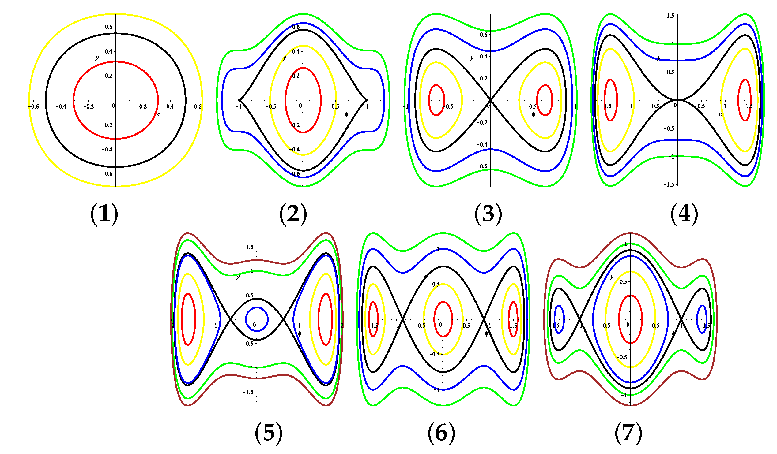
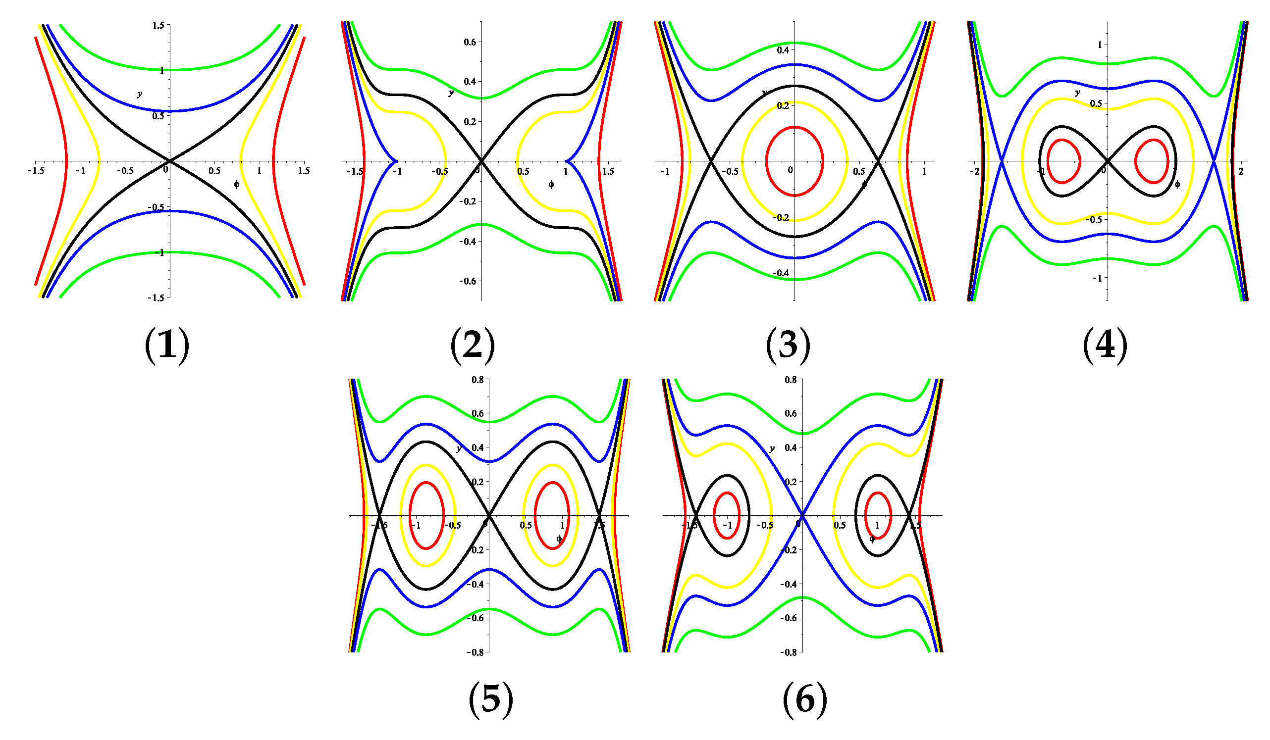
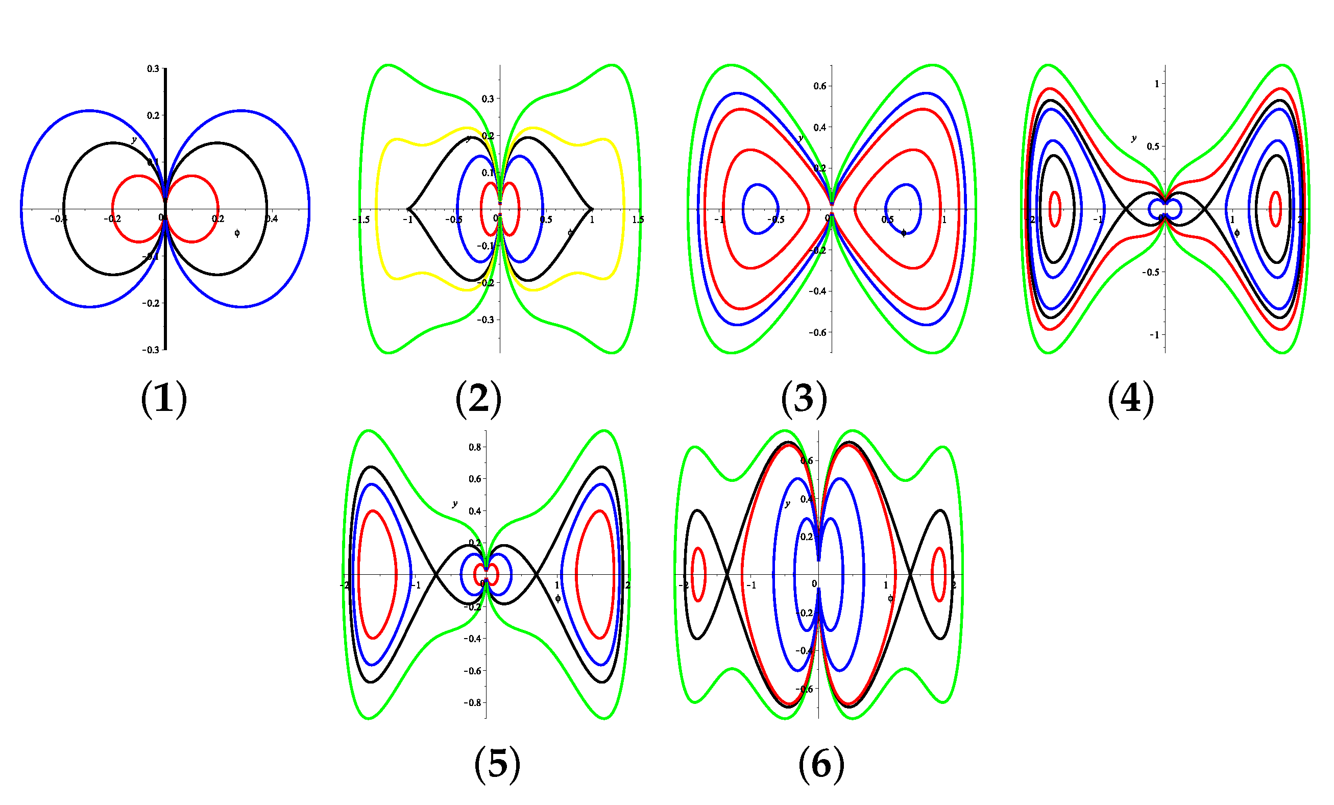
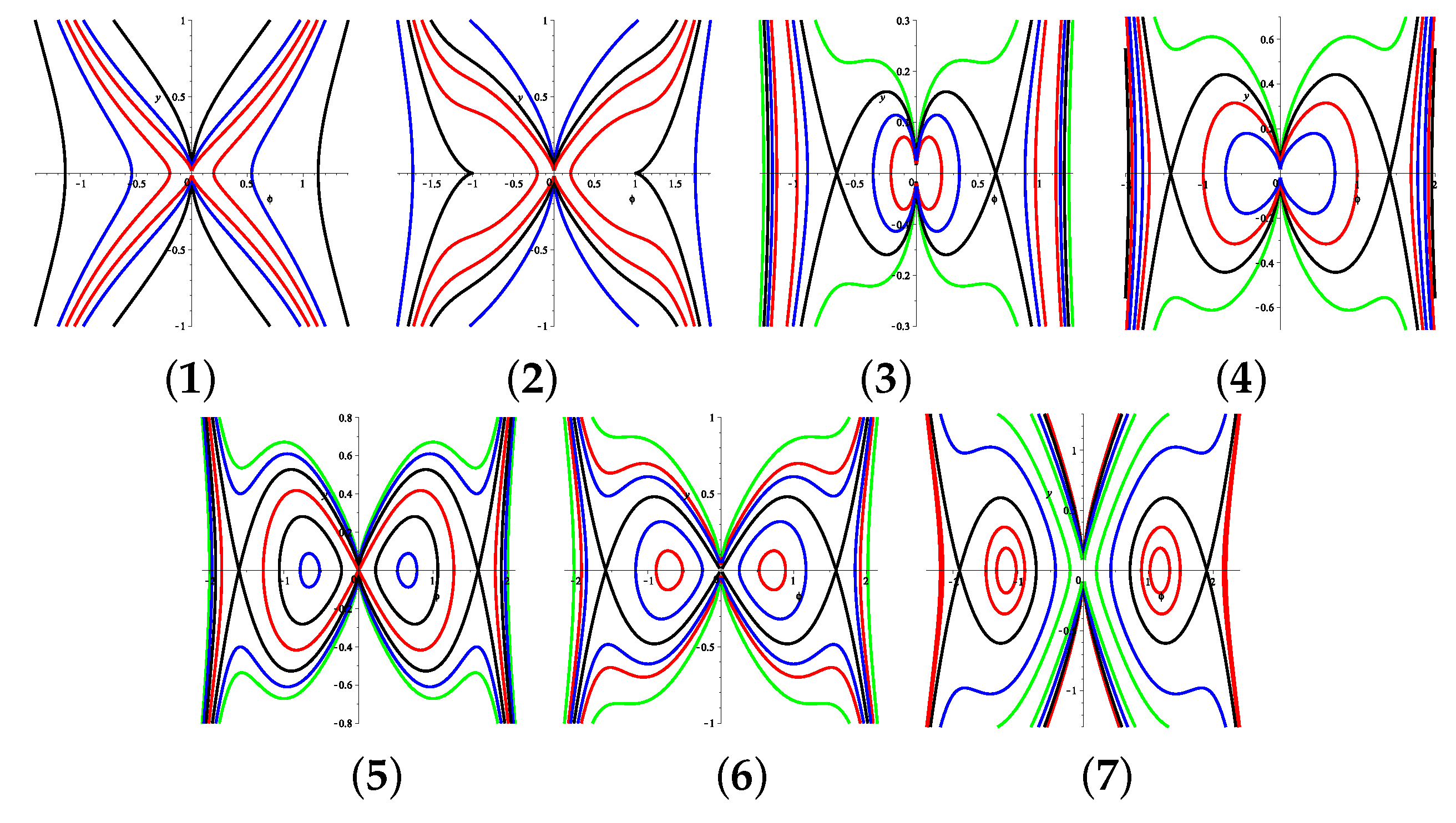
2. Bifurcations of Phase Portraits of System (5)

The associated regular system of (5) is
d ϕ d ζ = ( a 2 α ) ϕ y , d y d ζ = ( 2 α 4 β ) y 2 + ( ω + γ + a κ 2 ) ϕ 2 b ϕ 4 c ϕ 6 ,
where d ξ = ( a 2 α ) ϕ d ζ . Systems (5) and (11) have the same first integral. However, they have different time scales near the straight line ϕ = 0 (see [31]).
Firstly, we analyze the number of equilibrium points and their parametric regions. Obviously, when Δ = b 2 + 4 c ( ω + γ + a κ 2 ) > 0 , ϕ 2 = b ± Δ 2 c make c ϕ 4 + b ϕ 2 ( ω + γ + a κ 2 ) = 0 . Then, we have the following conclusions:
1. System (11) has only one equilibrium point E 0 ( 0 , 0 ) in the ϕ -axis if Δ < 0 ; or Δ > 0 , c > 0 , b > 0 , ω + γ + a κ 2 0 ; or Δ > 0 , c < 0 , b < 0 , ω + γ + a κ 2 0 ; or Δ = 0 , b c > 0 .
2. System (11) has three equilibrium points E 0 ( 0 , 0 ) , E 1 b + Δ 2 c , 0 and E 2 b + Δ 2 c , 0 in the ϕ -axis if Δ > 0 , c > 0 , ω + γ + a κ 2 > 0 ; System (11) has three equilibrium points E 0 ( 0 , 0 ) , E 3 b Δ 2 c , 0 and E 4 b Δ 2 c , 0 in the ϕ -axis if Δ > 0 , c < 0 , ω + γ + a κ 2 < 0 ; System (11) has three equilibrium points E 0 ( 0 , 0 ) , E 5 b 2 c , 0 and E 6 b 2 c , 0 in the ϕ -axis if Δ = 0 , b c < 0 .
3. System (11) has five equilibrium points E 0 ( 0 , 0 ) , E 1 b + Δ 2 c , 0 , E 2 b + Δ 2 c , 0   E 3 b Δ 2 c , 0 and E 4 b Δ 2 c , 0 in the ϕ -axis if Δ > 0 , c > 0 , b < 0 , ω + γ + a κ 2 < 0 ; or Δ > 0 , c < 0 , b > 0 , ω + γ + a κ 2 > 0 .
Secondly, in order to judge the type of an equilibrium point E j ( ϕ j , y j ) , we should know the sign of J ( ϕ j , y j ) = detM ( ϕ j , y j ) , where M is the coefficient matrix of the corresponding linear system of (11). When α = 2 β , we have
J ( 0 , 0 ) = ω + γ + a κ 2 a 2 α , J ± b + Δ 2 c , 0 = Δ ( Δ b ) c ( a 2 α ) ,
J ± b Δ 2 c , 0 = Δ ( Δ + b ) c ( a 2 α ) , J ± b 2 c , 0 = 0 .
when α 2 β , we have
J ( 0 , 0 ) = 0 , J ± b + Δ 2 c , 0 = ( a 2 α ) Δ ( Δ b ) 2 2 c 2 ,
J ± b Δ 2 c , 0 = ( a 2 α ) Δ ( Δ + b ) 2 2 c 2 , J ± b 2 c , 0 = 0 .
If J < 0 , then the equilibrium point E j ( ϕ j , y j ) is a saddle; if J > 0 , then it is a center; if J = 0 and the index of the equilibrium point is zero, then it is a cusp.
Next, we write that
h 0 = H ( 0 , 0 ) = 0 ( ) f o r 4 ( 2 β α ) ( a 2 α ) 0 ( < 0 ) ,
h 1 = H b + Δ 2 c , 0 , h 2 = H b + Δ 2 c , 0 , h 3 = H b Δ 2 c , 0 ,
h 4 = H b Δ 2 c , 0 , h 5 = H b 2 c , 0 , h 6 = H b 2 c , 0 ,
where H is given by (7). We have h 1 = h 2 , h 3 = h 4 , h 5 = h 6 , if 4 ( 2 β α ) ( a 2 α ) = 2 n , n N ; and h 1 = h 2 , h 3 = h 4 , h 5 = h 6 , if 4 ( 2 β α ) ( a 2 α ) = 2 n + 1 , n N .
In the following, we only discuss the case of c > 0 , because there is a similar conclusion when c < 0 . Using the aforementioned data, the bifurcations of the phase portraits of (5) are given in Figure 1, Figure 2, Figure 3, Figure 4, Figure 5 and Figure 6.

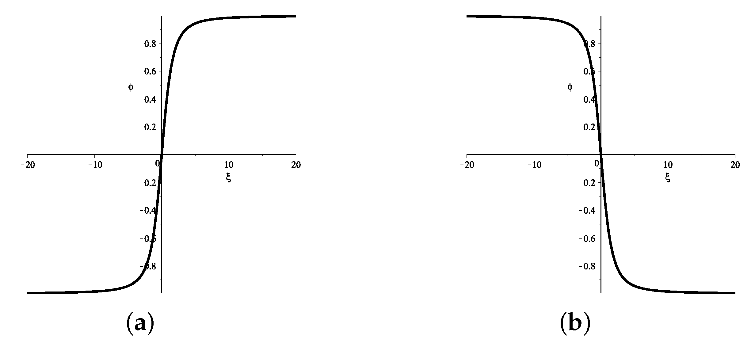
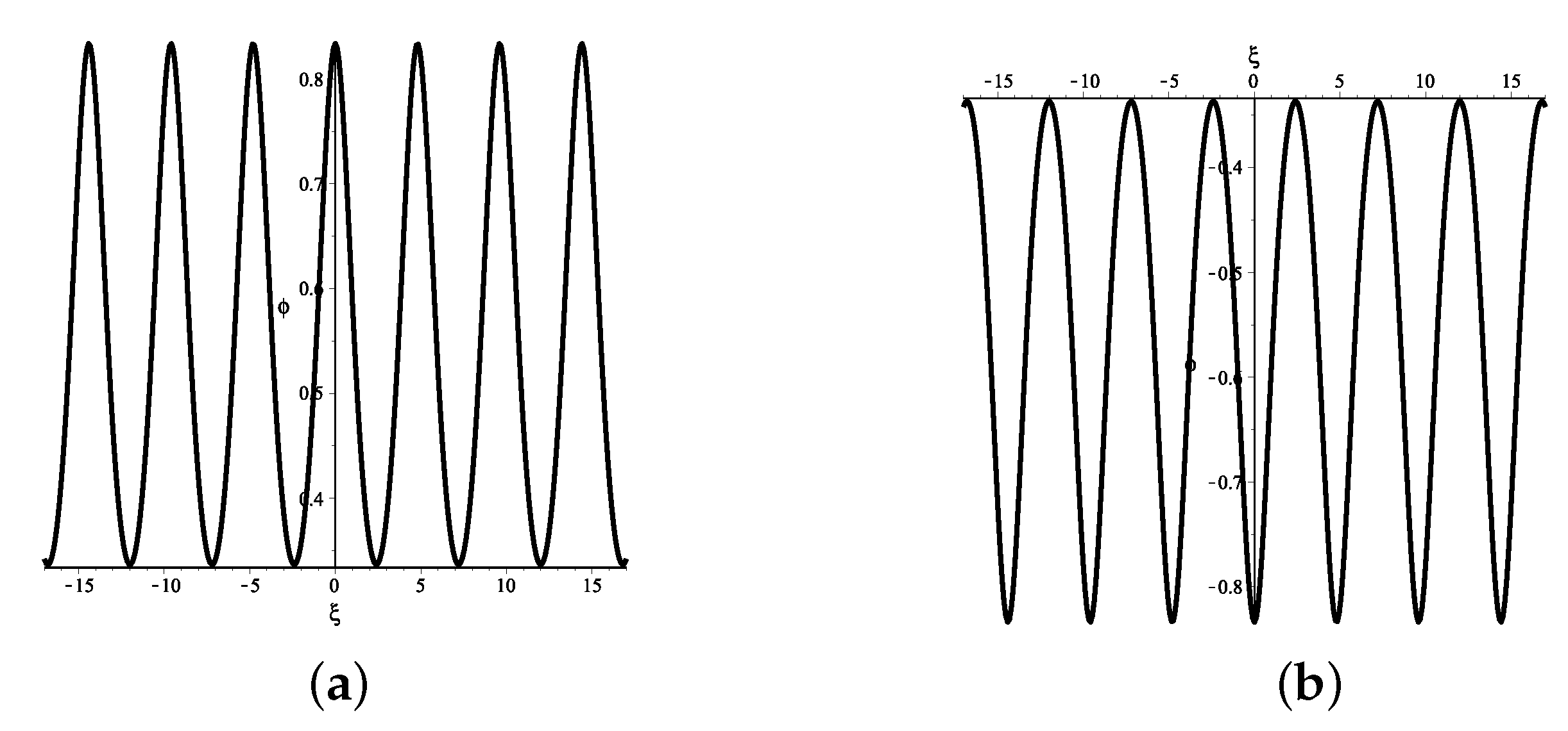
3. Expressions of the Traveling Wave Solutions of System (5) if C > 0 , α = 2 β

Currently, through integral calculation, we compute the exact parametric expressions of the traveling wave solutions if c > 0 , α = 2 β . According to Equation (7) and the first equation of system (5), we derive the following expression:
ξ = ϕ 0 ϕ d ϕ y ( ϕ ) = ϕ 0 ϕ ± d ϕ c 3 ( 2 α a ) ϕ 6 + b 2 ( 2 α a ) ϕ 4 + ω + γ + a κ 2 a 2 α ϕ 2 + h .

3.1. The Parameter Condition of A 2 α > 0 , Δ = 0 , B < 0 (See Figure 1(2))

In formula (7), if H ( ϕ , y ) = h 5 , there are two heteroclinic orbits, which encircle the equilibrium point E 0 and link the saddle points E 5 and E 6 . These two heteroclinic orbits correspond to kink and anti-kink wave solutions, respectively. Here, we have y 2 = c 3 ( a 2 α ) b 2 c ϕ 3 ϕ + b 2 c 3 . Combined with the integral formula (12), we get the expressions of the kink wave solution as (see Figure 7a)
ϕ ( ξ ) = b 3 ξ 2 24 c 2 ( 2 α a ) 2 c b 2 ξ 2 , ξ ( , 0 ] , b 3 ξ 2 24 c 2 ( 2 α a ) 2 c b 2 ξ 2 , ξ [ 0 , + ) ,
and the anti-kink wave solutions as (see Figure 7b):
ϕ ( ξ ) = b 3 ξ 2 24 c 2 ( 2 α a ) 2 c b 2 ξ 2 , ξ ( , 0 ] , b 3 ξ 2 24 c 2 ( 2 α a ) 2 c b 2 ξ 2 , ξ [ 0 , + ) .
From Equations (13) and (14), we deduce the expressions of two exact solutions of Equation (1) as
u ( x , t ) = b 3 ( x δ v t δ ) 2 24 c 2 δ 2 ( 2 α a ) 2 c b 2 ( x δ v t δ ) 2 e i η ( x , t ) , 1 δ ( x δ v t δ ) ( , 0 ] , b 3 ( x δ v t δ ) 2 24 c 2 δ 2 ( 2 α a ) 2 c b 2 ( x δ v t δ ) 2 e i η ( x , t ) , 1 δ ( x δ v t δ ) [ 0 , + ) ,
and
u ( x , t ) = b 3 ( x δ v t δ ) 2 24 c 2 δ 2 ( 2 α a ) 2 c b 2 ( x δ v t δ ) 2 e i η ( x , t ) , 1 δ ( x δ v t δ ) ( , 0 ] , b 3 ( x δ v t δ ) 2 24 c 2 δ 2 ( 2 α a ) 2 c b 2 ( x δ v t δ ) 2 e i η ( x , t ) , 1 δ ( x δ v t δ ) [ 0 , + ) .

3.2. The Parameter Condition of A 2 α > 0 , Δ > 0 , ω + γ + a κ 2 > 0 (See Figure 1(3))

(i) In formula (7), if H ( ϕ , y ) = h , h ( h 1 , h 0 ) , there are two families of periodic orbits, which respectively encircle the equilibrium points E 1 and E 2 . These two families of periodic orbits correspond to two periodic wave solutions of system (5). At present, y 2 = 4 c 3 ( a 2 α ) ( r 1 ϕ 2 ) ( ϕ 2 r 2 ) ( ϕ 2 r 3 ) , where r 1 > r 2 > 0 > r 3 . After calculation, we get the expressions of the two periodic wave solutions as (see Figure 8)
ϕ ( ξ ) = ± r 1 ( r 2 r 3 ) + r 3 ( r 1 r 2 ) sn 2 ( g 1 ξ , k 1 ) r 2 r 3 + ( r 1 r 2 ) sn 2 ( g 1 ξ , k 1 ) ,
where g 1 = c r 1 ( r 2 r 3 ) 3 ( a 2 α ) , k 1 2 = r 3 ( r 2 r 1 ) r 1 ( r 2 r 3 ) .
Thus, the two exact solutions of Equation (1) are given as
u ( x , t ) = ± r 1 ( r 2 r 3 ) + r 3 ( r 1 r 2 ) sn 2 ( g 1 1 δ ( x δ v t δ ) , k 1 ) r 2 r 3 + ( r 1 r 2 ) sn 2 ( g 1 1 δ ( x δ v t δ ) , k 1 ) e i η ( x , t ) .
(ii) In formula (7), if H ( ϕ , y ) = h 0 , there are two homoclinic orbits, which respectively encircle the equilibrium points E 1 and E 2 . The traveling wave solutions of the two homoclinic orbits are two solitary wave solutions of system (5). And, y 2 = 4 c 3 ( a 2 α ) ( r 1 ϕ 2 ) ϕ 2 ( ϕ 2 r 2 ) , where r 1 > 0 > r 2 . Thus, we obtain the parametric representations of the solitary wave solutions (see Figure 9)
ϕ ( ξ ) = ± 2 r 1 r 2 r 1 + r 2 + ( r 2 r 1 ) cosh ( g 2 ξ ) ,
where g 2 = 4 c r 1 r 2 3 ( 2 α a ) .
So, the two exact solutions of Equation (1) are given as
u ( x , t ) = ± 2 r 1 r 2 r 1 + r 2 + ( r 2 r 1 ) cosh ( g 2 1 δ ( x δ v t δ ) ) e i η ( x , t ) .

3.3. The Parameter Condition of A 2 α > 0 , Δ > 0 , B < 0 , ω + γ + a κ 2 = 0 (See Figure 1(4))

(i) There exist two families of periodic orbits when H ( ϕ , y ) = h , h ( h 1 , h 0 ) , which correspond to two periodic wave solutions of system (5). They have the same expressions as Equation (17).
(ii) In formula (7), if H ( ϕ , y ) = h 0 , there are two homoclinic orbits, which respectively encircle the equilibrium points E 1 and E 2 . The traveling wave solutions of the two homoclinic orbits are two solitary wave solutions of system (5). And, y 2 = 4 c 3 ( a 2 α ) ( r 1 ϕ 2 ) ϕ 4 , where r 1 > 0 . Thus, we obtain the parametric representations of the solitary wave solutions (see Figure 10):
ϕ ( ξ ) = ± 3 r 1 ( a 2 α ) 3 ( a 2 α ) + c r 1 2 ξ 2 .
So, the two exact solutions of Equation (1) are given as
u ( x , t ) = ± 3 r 1 ( a 2 α ) 3 ( a 2 α ) + c r 1 2 1 δ 2 ( x δ v t δ ) 2 e i η ( x , t ) .

3.4. The Parameter Condition of A 2 α > 0 , Δ > 0 , 3 b 2 16 c < b < 0 , ω + γ + a κ 2 < 0 (See Figure 1(5))

(i) There exist two families of periodic orbits when H ( ϕ , y ) = h , h ( h 1 , h 0 ] , which correspond to two periodic wave solutions of system (5). Their expressions are identical to Equation (17).
(ii) In formula (7), if H ( ϕ , y ) = h , h ( h 0 , h 3 ) , there are three families of periodic orbits, which respectively encircle the equilibrium points E 0 , E 1 and E 2 . For the periodic orbits surrounding the equilibrium point E 0 , we have y 2 = 4 c 3 ( a 2 α ) ( r 1 ϕ 2 ) ( r 2 ϕ 2 ) ( r 3 ϕ 2 ) . Then, we compute the representation of the periodic wave solution of system (5) (see Figure 11a)
ϕ ( ξ ) = r 2 r 3 r 2 r 3 sn 2 ( g 3 ξ , k 2 ) r 2 r 3 sn 2 ( g 3 ξ , k 2 ) , ξ ( 4 n + 1 ) ξ 1 , ( 4 n + 3 ) ξ 1 , r 2 r 3 r 2 r 3 sn 2 ( g 3 ξ , k 2 ) r 2 r 3 sn 2 ( g 3 ξ , k 2 ) , ξ 4 n ξ 1 , ( 4 n + 1 ) ξ 1 ( 4 n + 3 ) ξ 1 , ( 4 n + 4 ) ξ 1 ,
where g 3 = c r 2 ( r 1 r 3 ) 3 ( a 2 α ) , k 2 2 = r 3 ( r 1 r 2 ) r 2 ( r 1 r 3 ) , ξ 1 = 1 g 3 sn 1 ( 1 , k 2 ) , n Z .
For the periodic orbits surrounding the equilibrium points E 1 and E 2 , we have y 2 = 4 c 3 ( a 2 α ) ( r 1 ϕ 2 ) ( ϕ 2 r 2 ) ( ϕ 2 r 3 ) , where r 1 > r 2 > r 3 > 0 . Then, the expressions of the two periodic wave solutions are derived as (see Figure 11b,c)
ϕ ( ξ ) = ± r 1 r 2 r 2 + ( r 1 r 2 ) sn 2 ( g 3 ξ , k 2 ) .
Subsequently, the three exact periodic wave solutions of Equation (1) are given as
u ( x , t ) = r 2 r 3 r 2 r 3 sn 2 ( g 3 1 δ ( x δ v t δ ) , k 2 ) r 2 r 3 sn 2 ( g 3 1 δ ( x δ v t δ ) , k 2 ) e i η ( x , t ) , 1 δ ( x δ v t δ ) ( 4 n + 1 ) ξ 1 , ( 4 n + 3 ) ξ 1 , r 2 r 3 r 2 r 3 sn 2 ( g 3 1 δ ( x δ v t δ ) , k 2 ) r 2 r 3 sn 2 ( g 3 1 δ ( x δ v t δ ) , k 2 ) e i η ( x , t ) , 1 δ ( x δ v t δ ) 4 n ξ 1 , ( 4 n + 1 ) ξ 1 ( 4 n + 3 ) ξ 1 , ( 4 n + 4 ) ξ 1 ,
and
u ( x , t ) = ± r 1 r 2 r 2 + ( r 1 r 2 ) sn 2 ( g 3 1 δ ( x δ v t δ ) , k 2 ) e i η ( x , t ) .
(iii) In formula (7), if H ( ϕ , y ) = h 3 , there are two homoclinic orbits encircling the equilibrium points E 1 and E 2 , and two heteroclinic orbits linking two saddle points E 3 and E 4 . For the two homoclinic orbits, we have y 2 = 4 c 3 ( a 2 α ) ( r 1 ϕ 2 ) ϕ 2 b Δ 2 c 2 . Then, the expressions of the traveling wave solutions are derived as (see Figure 12)
ϕ ( ξ ) = ± r 1 ( b + Δ ) ( 1 + cosh ( g 4 ξ ) ) 2 ( b + Δ ) + 2 c r 1 ( 1 cosh ( g 4 ξ ) ) ,
where g 4 = ( b + Δ ) ( 2 c r 1 + b + Δ ) 3 c ( 2 α a ) .
For the two heteroclinic orbits, we have y 2 = 4 c 3 ( a 2 α ) ( r 1 ϕ 2 ) b Δ 2 c ϕ 2 2 , where r 1 > b Δ 2 c > 0 . Then, the the expression of the kink wave solution is given as (see Figure 13a)
ϕ ( ξ ) = r 1 ( b + Δ ) ( 1 cosh ( g 4 ξ ) ) 2 ( b + Δ ) + 2 c r 1 ( 1 + cosh ( g 4 ξ ) ) , ξ ( , 0 ] , r 1 ( b + Δ ) ( 1 cosh ( g 4 ξ ) ) 2 ( b + Δ ) + 2 c r 1 ( 1 + cosh ( g 4 ξ ) ) , ξ [ 0 , + ) ,
and the the expression of the anti-kink wave solution is given as (see Figure 13b)
ϕ ( ξ ) = r 1 ( b + Δ ) ( 1 cosh ( g 4 ξ ) ) 2 ( b + Δ ) + 2 c r 1 ( 1 + cosh ( g 4 ξ ) ) , ξ ( , 0 ] , r 1 ( b + Δ ) ( 1 cosh ( g 4 ξ ) ) 2 ( b + Δ ) + 2 c r 1 ( 1 + cosh ( g 4 ξ ) ) , ξ [ 0 , + ) .
So, Equation (1) has the following four exact solutions:
u ( x , t ) = ± r 1 ( b + Δ ) ( 1 + cosh ( g 4 1 δ ( x δ v t δ ) ) ) 2 ( b + Δ ) + 2 c r 1 ( 1 cosh ( g 4 1 δ ( x δ v t δ ) ) ) e i η ( x , t ) ,
u ( x , t ) = r 1 ( b + Δ ) ( 1 cosh ( g 4 1 δ ( x δ v t δ ) ) ) 2 ( b + Δ ) + 2 c r 1 ( 1 + cosh ( g 4 1 δ ( x δ v t δ ) ) ) e i η ( x , t ) , 1 δ ( x δ v t δ ) ( , 0 ] , r 1 ( b + Δ ) ( 1 cosh ( g 4 1 δ ( x δ v t δ ) ) ) 2 ( b + Δ ) + 2 c r 1 ( 1 + cosh ( g 4 1 δ ( x δ v t δ ) ) ) e i η ( x , t ) , 1 δ ( x δ v t δ ) [ 0 , + ) ,
and
u ( x , t ) = r 1 ( b + Δ ) ( 1 cosh ( g 4 1 δ ( x δ v t δ ) ) ) 2 ( b + Δ ) + 2 c r 1 ( 1 + cosh ( g 4 1 δ ( x δ v t δ ) ) ) e i η ( x , t ) , 1 δ ( x δ v t δ ) ( , 0 ] , r 1 ( b + Δ ) ( 1 cosh ( g 4 1 δ ( x δ v t δ ) ) ) 2 ( b + Δ ) + 2 c r 1 ( 1 + cosh ( g 4 1 δ ( x δ v t δ ) ) ) e i η ( x , t ) , 1 δ ( x δ v t δ ) [ 0 , + ) .

3.5. The Parameter Condition of A 2 α > 0 , Δ > 0 , B = 3 b 2 16 c , ω + γ + a κ 2 < 0 (See Figure 1(6))

(i) In formula (7), if H ( ϕ , y ) = h , h ( h 0 , h 3 ) , there are three families of periodic orbits. The expressions of the traveling wave solutions of these curves are identical to Equations (23) and (24).
(ii) In formula (7), if H ( ϕ , y ) = h 3 , there are two homoclinic orbits encircling the equilibrium points E 1 and E 2 , and two heteroclinic orbits linking two saddle points E 3 and E 4 . The expressions of the traveling wave solutions of these curves are identical to Equations (27)–(29).

3.6. The Parameter Condition of A 2 α > 0 , Δ > 0 , B < 3 b 2 16 c , ω + γ + a κ 2 < 0 (See Figure 1(7))

(i) In formula (7), if H ( ϕ , y ) = h , h ( h 1 , h 3 ) , there are three families of periodic orbits. The expressions of the traveling wave solutions of these curves are are identical to Equations (23) and (24).
(ii) In formula (7), if H ( ϕ , y ) = h 3 , there are two homoclinic orbits encircling the equilibrium points E 1 and E 2 and two heteroclinic orbits linking two saddle points E 3 and E 4 . The expressions of the traveling wave solutions of these curves are identical to Equations (27)–(29).

3.7. The Parameter Condition of Δ > 0 , ω + γ + a κ 2 > 0 or Δ > 0 , B < 0 , ω + γ + a κ 2 = 0 (See Figure 2(3))

(i) In formula (7), if H ( ϕ , y ) = h , h ( h 0 , h 1 ) , there is a family of periodic orbits, which encircle the equilibrium point E 0 . We have y 2 = 4 c 3 ( 2 α a ) ( r 1 ϕ 2 ) ( r 2 ϕ 2 ) ( ϕ 2 r 3 ) , where r 1 > r 2 > 0 > r 3 . Then, the parametric representation of the periodic wave solution is given as follows (see Figure 14):
ϕ ( ξ ) = r 1 r 2 r 1 r 2 sn 2 ( g 5 ξ , k 3 ) r 1 r 2 sn 2 ( g 5 ξ , k 3 ) , ξ ( 4 n + 1 ) ξ 2 , ( 4 n + 3 ) ξ 2 , r 1 r 2 r 1 r 2 sn 2 ( g 5 ξ , k 3 ) r 1 r 2 sn 2 ( g 5 ξ , k 3 ) , ξ 4 n ξ 2 , ( 4 n + 1 ) ξ 2 ( 4 n + 3 ) ξ 2 , ( 4 n + 4 ) ξ 2 ,
where g 5 = c r 1 ( r 3 r 2 ) 3 ( a 2 α ) , k 3 2 = r 2 ( r 1 r 3 ) r 1 ( r 2 r 3 ) , ξ 2 = 1 g 5 sn 1 ( 1 , k 3 ) , n Z .
Therefore, the exact solution of Equation (1) is given as follows:
u ( x , t ) = r 1 r 2 r 1 r 2 sn 2 ( g 5 1 δ ( x δ v t δ ) , k 3 ) r 1 r 2 sn 2 ( g 5 1 δ ( x δ v t δ ) , k 3 ) e i η ( x , t ) , 1 δ ( x δ v t δ ) ( 4 n + 1 ) ξ 2 , ( 4 n + 3 ) ξ 2 , r 1 r 2 r 1 r 2 sn 2 ( g 5 1 δ ( x δ v t δ ) , k 3 ) r 1 r 2 sn 2 ( g 5 1 δ ( x δ v t δ ) , k 3 ) e i η ( x , t ) , 1 δ ( x δ v t δ ) 4 n ξ 2 , ( 4 n + 1 ) ξ 2 ( 4 n + 3 ) ξ 2 , ( 4 n + 4 ) ξ 2 .
(ii) In formula (7), if H ( ϕ , y ) = h 1 , there are two heteroclinic orbits, which encircle the equilibrium point E 0 and link the saddle points E 1 and E 2 . We have y 2 = 4 c 3 ( 2 α a ) b + Δ 2 c ϕ 2 2 ( ϕ 2 r 1 ) , where b + Δ 2 c > 0 > r 1 . Then, the parametric representations of the kink and anti-kink wave solutions are given as (see Figure 15)
ϕ ( ξ ) = r 1 ( Δ b ) ( 1 cosh ( g 6 ξ ) ) 2 ( Δ b ) 2 c r 1 ( 1 + cosh ( g 6 ξ ) ) , ξ ( , 0 ] , r 1 ( Δ b ) ( 1 cosh ( g 6 ξ ) ) 2 ( Δ b ) 2 c r 1 ( 1 + cosh ( g 6 ξ ) ) , ξ [ 0 , + ) ,
and
ϕ ( ξ ) = r 1 ( Δ b ) ( 1 cosh ( g 6 ξ ) ) 2 ( Δ b ) 2 c r 1 ( 1 + cosh ( g 6 ξ ) ) , ξ ( , 0 ] , r 1 ( Δ b ) ( 1 cosh ( g 6 ξ ) ) 2 ( Δ b ) 2 c r 1 ( 1 + cosh ( g 6 ξ ) ) , ξ [ 0 , + ) ,
where g 6 = 2 ( Δ b ) 3 ( a 2 α ) r 1 b + Δ 2 c .
Thus, the exact expressions of solutions to Equation (1) are presented as
u ( x , t ) = r 1 ( Δ b ) ( 1 cosh ( g 6 1 δ ( x δ v t δ ) ) ) 2 ( Δ b ) 2 c r 1 ( 1 + cosh ( g 6 1 δ ( x δ v t δ ) ) ) e i η ( x , t ) , 1 δ ( x δ v t δ ) ( , 0 ] , r 1 ( Δ b ) ( 1 cosh ( g 6 1 δ ( x δ v t δ ) ) ) 2 ( Δ b ) 2 c r 1 ( 1 + cosh ( g 6 1 δ ( x δ v t δ ) ) ) e i η ( x , t ) , 1 δ ( x δ v t δ ) [ 0 , + ) ,
and
u ( x , t ) = r 1 ( Δ b ) ( 1 cosh ( g 6 1 δ ( x δ v t δ ) ) ) 2 ( Δ b ) 2 c r 1 ( 1 + cosh ( g 6 1 δ ( x δ v t δ ) ) ) e i η ( x , t ) , 1 δ ( x δ v t δ ) ( , 0 ] , r 1 ( Δ b ) ( 1 cosh ( g 6 1 δ ( x δ v t δ ) ) ) 2 ( Δ b ) 2 c r 1 ( 1 + cosh ( g 6 1 δ ( x δ v t δ ) ) ) e i η ( x , t ) , 1 δ ( x δ v t δ ) [ 0 , + ) .

3.8. The Parameter Condition of A 2 α < 0 , Δ > 0 , 3 b 2 16 c < b < 0 , ω + γ + a κ 2 < 0 (See Figure 2(4))

(i) In formula (7), if H ( ϕ , y ) = h , h ( h 3 , h 0 ) , there are two families of periodic orbits, which respectively encircle the equilibrium points E 3 and E 4 . We have y 2 = 4 c 3 ( 2 α a ) ( r 3 ϕ 2 ) ( r 1 ϕ 2 ) ( ϕ 2 r 2 ) , where r 3 > r 1 > r 2 > 0 . Then, we derive the parametric representations of the periodic wave solutions are given as (see Figure 16)
ϕ ( ξ ) = ± r 1 ( r 2 r 3 ) + r 3 ( r 1 r 2 ) sn 2 ( g 7 ξ , k 4 ) r 2 r 3 + ( r 1 r 2 ) sn 2 ( g 7 ξ , k 4 ) ,
where g 7 = c r 1 ( r 2 r 3 ) 3 ( a 2 α ) , k 4 2 = r 3 ( r 1 r 2 ) r 1 ( r 3 r 2 ) .
Thus, the exact expressions of solutions to Equation (1) are presented as
u ( x , t ) = ± r 1 ( r 2 r 3 ) + r 3 ( r 1 r 2 ) sn 2 ( g 7 1 δ ( x δ v t δ ) , k 4 ) r 2 r 3 + ( r 1 r 2 ) sn 2 ( g 7 1 δ ( x δ v t δ ) , k 4 ) e i η ( x , t ) .
(ii) In formula (7), if H ( ϕ , y ) = h 0 , there are two homoclinic orbits, which respectively encircle the equilibrium points E 3 and E 4 . We have y 2 = 4 c 3 ( 2 α a ) ( r 1 ϕ 2 ) ( r 2 ϕ 2 ) ϕ 2 , where r 1 > r 2 > 0 . Then, we derive the parametric expressions of the solitary wave solutions as (see Figure 17)
ϕ ( ξ ) = ± 2 r 1 r 2 r 1 + r 2 + ( r 1 r 2 ) cosh ( g 8 ξ ) ,
where g 8 = 4 c r 1 r 2 3 ( 2 α a ) .
Thus, the exact expressions of two solitary wave solutions to Equation (1) are presented as
u ( x , t ) = ± 2 r 1 r 2 r 1 + r 2 + ( r 1 r 2 ) cosh ( g 8 1 δ ( x δ v t δ ) ) e i η ( x , t ) .
(iii) In formula (7), if H ( ϕ , y ) = h , h ( h 0 , h 1 ) , there is a family of periodic orbits. The expressions of the traveling wave solutions of these curves are identical to Equation (33).
(iv) The curves H ( ϕ , y ) = h 1 correspond to two heteroclinic orbits. The parametric expressions of the traveling wave solutions of these curves are the same as Equations (35) and (36).

3.9. The Parameter Condition of A 2 α < 0 , Δ > 0 , B = 3 b 2 16 c , ω + γ + a κ 2 < 0 (See Figure 2(5))

(i) In formula (7), if H ( ϕ , y ) = h , h ( h 3 , h 0 ) , there are two families of periodic orbits. The expressions of the traveling wave solutions of these curves are identical to Equation (39).
(ii) In formula (7), if H ( ϕ , y ) = h 0 , there are four heteroclinic orbits, which encircle the equilibrium points E 3 and E 4 and link the saddle points E 0 , E 1 and E 2 . We have y 2 = 4 c 3 ( 2 α a ) b + Δ 2 c ϕ 2 2 ϕ 2 . The heteroclinic orbit in the first quadrant corresponds to a kink wave solution, and the parametric expression of the kink wave solution is given as (see Figure 18a)
ϕ ( ξ ) = b + Δ 4 c b + Δ 4 c tanh ln 3 b + Δ 4 c g 9 ξ ,
where g 9 = 4 c 3 ( 2 α a ) . The heteroclinic orbit in the forth quadrant corresponds to an anti-kink wave solution, and the parametric representation of the anti-kink wave solution is given as (see Figure 18b)
ϕ ( ξ ) = b + Δ 4 c b + Δ 4 c tanh ln 3 + b + Δ 4 c g 9 ξ .
The heteroclinic orbit in the second quadrant corresponds to a kink wave solution, and the parametric representation of the kink wave solution is given as (see Figure 18c)
ϕ ( ξ ) = b + Δ 4 c b + Δ 4 c tanh ln 3 + b + Δ 4 c g 9 ξ .
The heteroclinic orbit in the third quadrant corresponds to a anti-kink wave solution, and the parametric representation of the anti-kink wave solution is given as (see Figure 18d)
ϕ ( ξ ) = b + Δ 4 c b + Δ 4 c tanh ln 3 b + Δ 4 c g 9 ξ .
Thus, the exact expressions of solutions to Equation (1) are presented as
u ( x , t ) = b + Δ 4 c b + Δ 4 c tanh ln 3 b + Δ 4 c g 9 1 δ ( x δ v t δ ) e i η ( x , t ) ,
u ( x , t ) = b + Δ 4 c b + Δ 4 c tanh ln 3 + b + Δ 4 c g 9 1 δ ( x δ v t δ ) e i η ( x , t ) ,
and
u ( x , t ) = b + Δ 4 c b + Δ 4 c tanh ln 3 b + Δ 4 c g 9 1 δ ( x δ v t δ ) e i η ( x , t ) .

3.10. The Parameter Condition of A 2 α < 0 , Δ > 0 , B < 3 b 2 16 c , ω + γ + a κ 2 < 0 (See Figure 2(6))

(i) In formula (7), if H ( ϕ , y ) = h , h ( h 3 , h 1 ) , there are two families of periodic orbits. The expressions of the traveling wave solutions of these curves are identical to Equation (39).
(ii) In formula (7), if H ( ϕ , y ) = h 1 , there are two homoclinic orbits, which respectively encircle the equilibrium points E 3 and E 4 . We have y 2 = 4 c 3 ( 2 α a ) b + Δ 2 c ϕ 2 2 ( ϕ 2 r 1 ) , where b + Δ 2 c > r 1 > 0 . Then, the parametric representations of the solitary wave solutions are given as (see Figure 19)
ϕ ( ξ ) = ± r 1 ( Δ b ) ( 1 + cosh ( g 10 ξ ) ) 2 ( Δ b ) + 2 c r 1 ( cosh ( g 10 ξ ) 1 ) ,
where g 10 = 2 ( Δ b ) 3 ( a 2 α ) r 1 b + Δ 2 c .
Thus, the exact expressions of solutions to Equation (1) are presented as
u ( x , t ) = ± r 1 ( Δ b ) ( 1 + cosh ( g 10 1 δ ( x δ v t δ ) ) ) 2 ( Δ b ) + 2 c r 1 ( cosh ( g 10 1 δ ( x δ v t δ ) ) 1 ) e i η ( x , t ) .

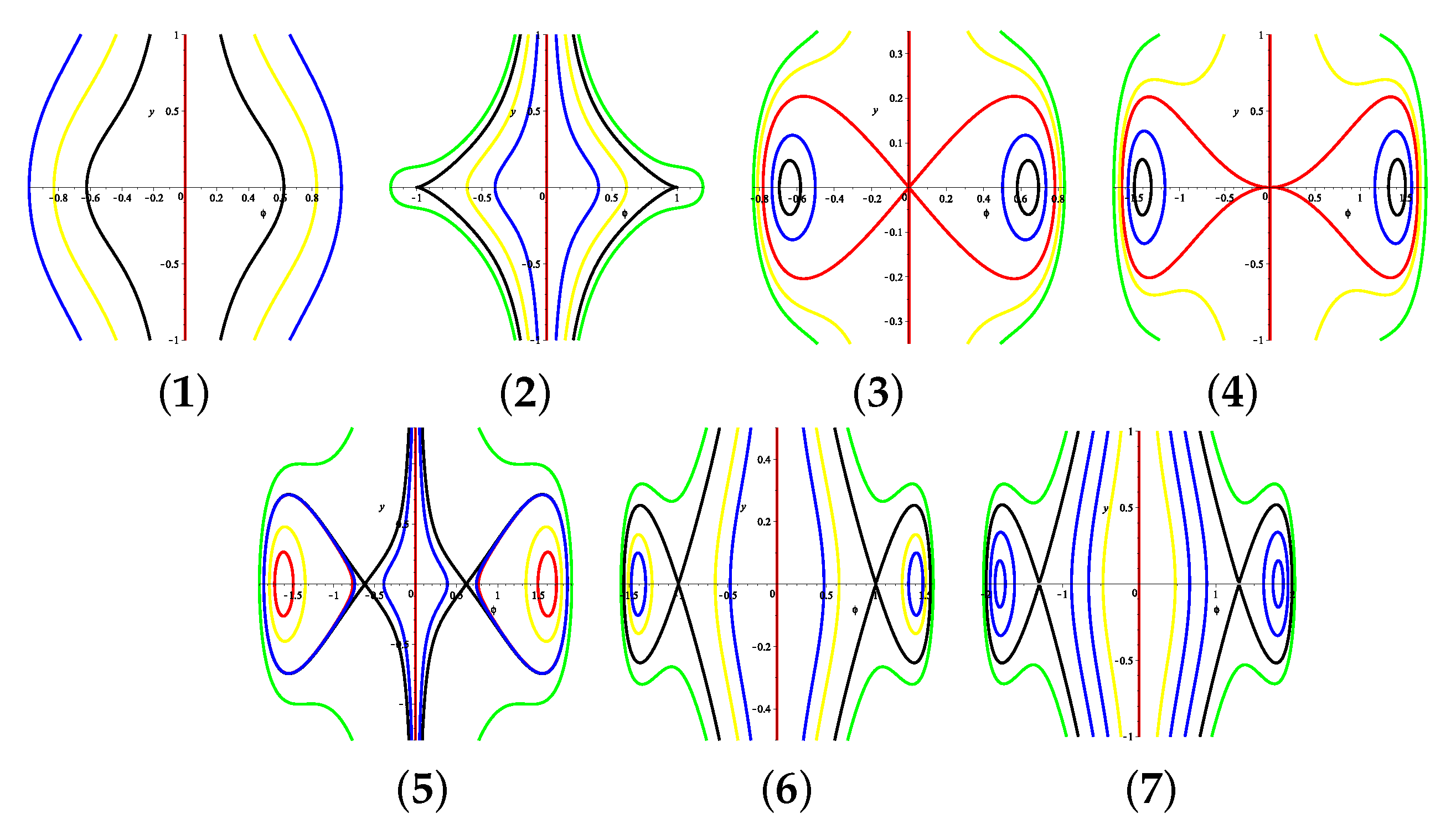
4. Expressions of the Traveling Wave Solutions of System Equation (5) under C > 0 , A = 4 β

Currently, through integral calculation, we compute the exact parametric expressions of the traveling wave solutions under c > 0 , a = 4 β . It follows from Equation (7) and the first equation of system (5) that
ξ = ϕ 0 ϕ ± | ϕ | d ϕ c 4 ( 2 α a ) ϕ 8 + b 3 ( 2 α a ) ϕ 6 + ω + γ + a κ 2 2 ( a 2 α ) ϕ 4 + h ϕ 0 ϕ ± | ϕ | d ϕ G ( ϕ ) .

4.1. The Parameter Condition of A 2 α > 0 , Δ > 0 , ω + γ + a κ 2 > 0 (See Figure 3(3))

(i) In formula (7), if H ( ϕ , y ) = h , h ( h 1 , h 0 ) , there are two families of periodic orbits, which respectively encircle the equilibrium points E 1 and E 2 . We have G ( ϕ ) = c 4 ( a 2 α ) ( r 1 ϕ 2 ) ( ϕ 2 r 2 ) ( ϕ 2 r 3 ) ( ϕ 2 r 4 ) , where r 1 > r 2 > 0 > r 3 > r 4 . Then, the expressions of the periodic wave solutions are derived as (see Figure 20)
ϕ ( ξ ) = ± r 1 ( r 2 r 4 ) + r 4 ( r 1 r 2 ) sn 2 ( g 11 ξ , k 5 ) r 2 r 4 + ( r 1 r 2 ) sn 2 ( g 11 ξ , k 5 ) ,
where g 11 = c ( r 1 r 3 ) ( r 2 r 4 ) 4 ( a 2 α ) , k 5 2 = ( r 1 r 2 ) ( r 3 r 4 ) ( r 1 r 3 ) ( r 2 r 4 ) .
Thus, the exact expressions of solutions to Equation (1) are presented as
u ( x , t ) = ± r 1 ( r 2 r 4 ) + r 4 ( r 1 r 2 ) sn 2 ( g 11 1 δ ( x δ v t δ ) , k 5 ) r 2 r 4 + ( r 1 r 2 ) sn 2 ( g 11 1 δ ( x δ v t δ ) , k 5 ) e i η ( x , t ) .
(ii) In formula (7), if H ( ϕ , y ) = h 0 , there are two homoclinic orbits, which respectively encircle the equilibrium points E 1 and E 2 . We have G ( ϕ ) = c a 2 α ( r 1 ϕ 2 ) ϕ 4 ( ϕ 2 r 2 ) , where r 1 > 0 > r 2 . Then, the parametric representations of the solitary wave solutions are given as (see Figure 21)
ϕ ( ξ ) = ± 2 r 1 r 2 r 1 + r 2 + ( r 2 r 1 ) cosh ( g 12 ξ ) ,
where g 12 = c r 1 r 2 2 α a .
Thus, the exact expressions of solutions to Equation (1) are presented as
u ( x , t ) = ± 2 r 1 r 2 r 1 + r 2 + ( r 2 r 1 ) cosh ( g 12 1 δ ( x δ v t δ ) ) e i η ( x , t ) .

4.2. The Parameter Condition of A 2 α > 0 , Δ > 0 , B < 0 , ω + γ + a κ 2 = 0 (See Figure 3(4))

(i) In formula (7), if H ( ϕ , y ) = h , h ( h 1 , h 0 ) , there are two families of periodic orbits, which respectively encircle the equilibrium points E 1 and E 2 . We have G ( ϕ ) = c 4 ( a 2 α ) ( r 1 ϕ 2 ) ( ϕ 2 r 2 ) ( ϕ 2 r 3 ) ( ϕ 2 r 3 ¯ ) , where r 1 > r 2 , r 3 and r 3 ¯ are complex. Then, the parametric representation of the periodic wave solution are given as (see Figure 22)
ϕ ( ξ ) = ± r 1 B 1 + r 2 A 1 + ( r 2 A 1 r 1 B 1 ) cn ( g 13 ξ , k 6 ) A 1 + B 1 + ( A 1 B 1 ) cn ( g 13 ξ , k 6 ) ,
where A 1 2 = ( r 1 r 3 ) ( r 1 r 3 ¯ ) , B 1 2 = ( r 2 r 3 ) ( r 2 r 3 ¯ ) , g 13 = c A 1 B 1 a 2 α , k 6 2 = ( r 1 r 2 ) 2 ( A 1 B 1 ) 2 4 A 1 B 1 .
Thus, the exact expressions of solutions to Equation (1) are presented as
u ( x , t ) = ± r 1 B 1 + r 2 A 1 + ( r 2 A 1 r 1 B 1 ) cn ( g 13 1 δ ( x δ v t δ ) , k 6 ) A 1 + B 1 + ( A 1 B 1 ) cn ( g 13 1 δ ( x δ v t δ ) , k 6 ) e i η ( x , t ) .
(ii) In formula (7), if H ( ϕ , y ) = h 0 , there are two homoclinic orbits, which respectively encircle the equilibrium points E 1 and E 2 . We have G ( ϕ ) = c a 2 α ( r 1 ϕ 2 ) ϕ 6 , where r 1 > 0 . Then, the parametric representations of the solitary wave solutions are given as (see Figure 23)
ϕ ( ξ ) = ± 4 r 1 ( a 2 α ) 4 ( a 2 α ) + c r 1 2 ξ 2 .
Thus, the exact expressions of solutions to Equation (1) are presented as
u ( x , t ) = ± 4 r 1 ( a 2 α ) 4 ( a 2 α ) + c r 1 2 1 δ 2 ( x δ v t δ ) 2 e i η ( x , t ) .

4.3. The Parameter Condition of A 2 α > 0 , Δ > 0 , B < 0 , ω + γ + a κ 2 < 0 , H 1 = h 2 < h 0 < h 3 = h 4 (See Figure 3(5))

(i) In formula (7), if H ( ϕ , y ) = h , h ( h 1 , h 0 ) , there are two families of periodic orbits. The expressions of the traveling wave solutions of these curves are identical to Equations (56) and (58)
(ii) In formula (7), if H ( ϕ , y ) = h 0 , there are two families of periodic orbits, which respectively encircle the equilibrium points E 1 and E 2 . We have G ( ϕ ) = c 4 ( a 2 α ) ( r 1 ϕ 2 ) ( ϕ 2 r 2 ) ϕ 4 , where r 1 > r 2 > 0 . Then, the expressions of the periodic wave solutions are derived as (see Figure 24)
ϕ ( ξ ) = ± 2 r 1 r 2 r 1 + r 2 ( r 1 r 2 ) cos ( g 14 ξ ) ,
where g 14 = c r 1 r 2 a 2 α .
Thus, the exact expressions of solutions to Equation (1) are presented as
u ( x , t ) = ± 2 r 1 r 2 r 1 + r 2 ( r 1 r 2 ) cos ( g 14 1 δ ( x δ v t δ ) ) e i η ( x , t ) .
(iii) In formula (7), if H ( ϕ , y ) = h , h ( h 0 , h 3 ) , there are two families of periodic orbits respectively surrounding the equilibrium points E 1 and E 2 , and two families of open curves, which tend to the singular line ϕ = 0 under | y | . G ( ϕ ) = c 4 ( a 2 α ) ( r 1 ϕ 2 ) ( ϕ 2 r 2 ) ( ϕ 2 r 3 ) ( ϕ 2 r 4 ) applies to the two families of periodic orbits. Then, the expressions of the periodic wave solutions are derived as (see Figure 25)
ϕ ( ξ ) = ± r 1 ( r 2 r 4 ) + r 4 ( r 1 r 2 ) sn 2 ( g 15 ξ , k 7 ) r 2 r 4 + ( r 1 r 2 ) sn 2 ( g 15 ξ , k 7 ) ,
where g 15 = c ( r 1 r 3 ) ( r 2 r 4 ) 4 ( a 2 α ) , k 7 2 = ( r 1 r 2 ) ( r 3 r 4 ) ( r 1 r 3 ) ( r 2 r 4 ) .
G ( ϕ ) = c 4 ( a 2 α ) ( r 1 ϕ 2 ) ( r 2 ϕ 2 ) ( r 3 ϕ 2 ) ( ϕ 2 r 4 ) applies to the two families of open curves, where r 1 > r 2 > r 3 > 0 > r 4 . Then, the parametric representations of the compacton solutions are given as (see Figure 26)
ϕ ( ξ ) = ± r 3 ( r 4 r 2 ) + r 2 ( r 3 r 4 ) sn 2 ( g 15 ξ , k 7 ) r 4 r 2 + ( r 3 r 4 ) sn 2 ( g 15 ξ , k 7 ) , ξ ( ξ 3 , ξ 3 ) ,
where ξ 3 = 1 g 15 sn 1 r 3 ( r 2 r 4 ) r 2 ( r 3 r 4 ) , k 7 .
So, Equation (1) has the following four exact solutions:
u ( x , t ) = ± r 1 ( r 2 r 4 ) + r 4 ( r 1 r 2 ) sn 2 ( g 15 1 δ ( x δ v t δ ) , k 7 ) r 2 r 4 + ( r 1 r 2 ) sn 2 ( g 15 1 δ ( x δ v t δ ) , k 7 ) e i η ( x , t ) ,
and
u ( x , t ) = ± r 3 ( r 4 r 2 ) + r 2 ( r 3 r 4 ) sn 2 ( g 15 1 δ ( x δ v t δ ) , k 7 ) r 4 r 2 + ( r 3 r 4 ) sn 2 ( g 15 1 δ ( x δ v t δ ) , k 7 ) e i η ( x , t ) , 1 δ ( x δ v t δ ) ( ξ 3 , ξ 3 ) .
(iv) In formula (7), if H ( ϕ , y ) = h 3 , there are two homoclinic orbits, which respectively encircle the equilibrium points E 1 and E 2 . We have G ( ϕ ) = c 4 ( a 2 α ) ( r 1 ϕ 2 ) ϕ 2 b Δ 2 c 2 ( ϕ 2 r 2 ) , where r 1 > b Δ 2 c > 0 > r 2 . Then, the parametric representations of the solitary wave solutions are given as (see Figure 27)
ϕ ( ξ ) = ± 4 c r 1 r 2 + ( r 1 + r 2 ) ( b + Δ ) + ( r 1 r 2 ) ( b + Δ ) cosh ( g 16 ξ ) 2 c ( r 1 + r 2 ) + 2 ( b + Δ ) + 2 c ( r 2 r 1 ) cosh ( g 16 ξ ) ,
where g 16 = ( 2 c r 1 + b + Δ ) ( 2 c r 2 + b + Δ ) 4 c ( 2 α a ) .
Thus, the exact expressions of solutions to Equation (1) are presented as
u ( x , t ) = ± 4 c r 1 r 2 + ( r 1 + r 2 ) ( b + Δ ) + ( r 1 r 2 ) ( b + Δ ) cosh ( g 16 1 δ ( x δ v t δ ) ) 2 c ( r 1 + r 2 ) + 2 ( b + Δ ) + 2 c ( r 2 r 1 ) cosh ( g 16 1 δ ( x δ v t δ ) ) e i η ( x , t ) .

4.4. The Parameter Condition of A 2 α > 0 , Δ > 0 , B < 0 , ω + γ + a κ 2 < 0 , H 1 = h 2 = h 0 < h 3 = h 4 (See Figure 3(6))

(i) In formula (7), if H ( ϕ , y ) = h , h ( h 0 , h 3 ) , there are two families of periodic orbits and two families of open curves. The parametric representations of the traveling wave solutions of these curves are same as Equations (64) and (65).
(ii) The curves H ( ϕ , y ) = h 3 correspond to two homoclinic orbits. The parametric expressions of the traveling wave solutions of these curves are the same as Equations (68).

4.5. The Parameter Condition of A 2 α > 0 , Δ > 0 , B < 0 , ω + γ + a κ 2 < 0 , H 0 < h 1 = h 2 < h 3 = h 4 (See Figure 3(7))

(i) In formula (7), if H ( ϕ , y ) = h , h ( h 2 , h 3 ) , there are two families of periodic orbits and two families of open curves. The parametric representations of the traveling wave solutions of these curves are the same as Equations (64) and (65).
(ii) The curves H ( ϕ , y ) = h 3 correspond to two homoclinic orbits. The parametric expressions of the traveling wave solutions of these curves are the same as Equations (68).

4.6. The Parameter Condition of A 2 α < 0 , Δ > 0 , ω + γ + a κ 2 > 0 or Δ > 0 , B < 0 , ω + γ + a κ 2 = 0 (See Figure 4(3))

In formula (7), if H ( ϕ , y ) = h , h ( h 0 , h 1 ) , there are two families of open curves, which tend to the singular line ϕ = 0 when | y | . We have G ( ϕ ) = c 4 ( 2 α a ) ( r 1 ϕ 2 ) ( r 2 ϕ 2 ) ( ϕ 2 r 3 ) ( ϕ 2 r 4 ) , where r 1 > r 2 > 0 > r 3 > r 4 . Then, the parametric representations of the compacton solutions are given as (see Figure 28)
ϕ ( ξ ) = ± r 2 ( r 3 r 1 ) + r 1 ( r 2 r 3 ) sn 2 ( g 17 ξ , k 8 ) r 3 r 1 + ( r 2 r 3 ) sn 2 ( g 17 ξ , k 8 ) , ξ ( ξ 4 , ξ 4 ) ,
where g 17 = c ( r 3 r 1 ) ( r 2 r 4 ) 4 ( a 2 α ) , k 8 2 = ( r 2 r 3 ) ( r 1 r 4 ) ( r 1 r 3 ) ( r 2 r 4 ) , ξ 4 = 1 g 17 sn 1 r 2 ( r 1 r 3 ) r 1 ( r 2 r 3 ) , k 8 .
Thus, the exact expressions of solutions to Equation (1) are presented as
u ( x , t ) = ± r 2 ( r 3 r 1 ) + r 1 ( r 2 r 3 ) sn 2 ( g 17 1 δ ( x δ v t δ ) , k 8 ) r 3 r 1 + ( r 2 r 3 ) sn 2 ( g 17 1 δ ( x δ v t δ ) , k 8 ) e i η ( x , t ) , 1 δ ( x δ v t δ ) ( ξ 4 , ξ 4 ) .

4.7. The Parameter Condition of A 2 α < 0 , Δ > 0 , B < 0 , ω + γ + a κ 2 < 0 , H 3 = h 4 < h 0 < h 1 = h 2 (See Figure 4(4))

(i) In formula (7), if H ( ϕ , y ) = h , h ( h 3 , h 0 ) , there are two families of periodic orbits, which respectively encircle the equilibrium points E 3 and E 4 . We have G ( ϕ ) = c 4 ( 2 α a ) ( r 1 ϕ 2 ) ( r 2 ϕ 2 ) ( ϕ 2 r 3 ) ( ϕ 2 r 4 ) , where r 1 > r 2 > r 3 > 0 > r 4 . Then, the expressions of the periodic wave solutions are derived as (see Figure 29)
ϕ ( ξ ) = ± r 2 ( r 3 r 1 ) + r 1 ( r 2 r 3 ) sn 2 ( g 18 ξ , k 9 ) r 3 r 1 + ( r 2 r 3 ) sn 2 ( g 18 ξ , k 9 ) ,
where g 18 = c ( r 3 r 1 ) ( r 2 r 4 ) 4 ( a 2 α ) , k 9 2 = ( r 2 r 3 ) ( r 1 r 4 ) ( r 1 r 3 ) ( r 2 r 4 ) .
Thus, the exact expressions of solutions to Equation (1) are presented as
u ( x , t ) = ± r 2 ( r 3 r 1 ) + r 1 ( r 2 r 3 ) sn 2 ( g 18 1 δ ( x δ v t δ ) , k 9 ) r 3 r 1 + ( r 2 r 3 ) sn 2 ( g 18 1 δ ( x δ v t δ ) , k 9 ) e i η ( x , t ) .
(ii) In formula (7), if H ( ϕ , y ) = h 0 , there are two homoclinic orbits, which respectively encircle the equilibrium points E 3 and E 4 . We have G ( ϕ ) = c 2 α a ( r 1 ϕ 2 ) ( r 2 ϕ 2 ) ϕ 4 , where r 1 > r 2 > 0 . Then, the parametric representations of the solitary wave solutions are given as (see Figure 30)
ϕ ( ξ ) = ± 2 r 1 r 2 r 1 + r 2 + ( r 1 r 2 ) cosh ( g 19 ξ ) ,
where g 19 = c r 1 r 2 2 α a .
Thus, the exact expressions of solutions to Equation (1) are presented as
u ( x , t ) = ± 2 r 1 r 2 r 1 + r 2 + ( r 1 r 2 ) cosh ( g 19 1 δ ( x δ v t δ ) ) e i η ( x , t ) .
(iii) In formula (7), if H ( ϕ , y ) = h , h ( h 0 , h 1 ) , there are two families of open curves, which tend to the singular line ϕ = 0 under | y | . The traveling wave solutions of these curves are as (70).

4.8. The Parameter Condition of A 2 α < 0 , Δ > 0 , B < 0 , ω + γ + a κ 2 < 0 , H 3 = h 4 < h 0 = h 1 = h 2 (See Figure 4(5))

(i) In formula (7), if H ( ϕ , y ) = h , h ( h 3 , h 0 ) , there are two families of periodic orbits. The expressions of the traveling wave solutions of these curves are identical to Equation (72).
(ii) In formula (7), if H ( ϕ , y ) = h 0 , there are four heteroclinic orbits, which encircle the equilibrium points E 3 and E 4 and link the saddle points E 0 , E 1 and E 2 . Now, we have G ( ϕ ) = c 2 α a b + Δ 2 c ϕ 2 2 ϕ 4 . The heteroclinic orbit in the first quadrant corresponds to a kink wave solution, and the parametric expression of the kink wave solution is given as (see Figure 31a)
ϕ ( ξ ) = b + Δ 4 c b + Δ 4 c tanh ln 3 b + Δ 4 c g 20 ξ ,
where g 20 = c 2 α a .
The heteroclinic orbit in the forth quadrant corresponds to an anti-kink wave solution, and the parametric representation of the anti-kink wave solution is given as (see Figure 31b)
ϕ ( ξ ) = b + Δ 4 c b + Δ 4 c tanh ln 3 + b + Δ 4 c g 20 ξ .
The heteroclinic orbit in the second quadrant corresponds to a kink wave solution, and the parametric representation of the kink wave solution is given as (see Figure 31c)
ϕ ( ξ ) = b + Δ 4 c b + Δ 4 c tanh ln 3 + b + Δ 4 c g 20 ξ .
The heteroclinic orbit in the third quadrant corresponds to an anti-kink wave solution, and the parametric representation of the anti-kink wave solution is given as (see Figure 31d)
ϕ ( ξ ) = b + Δ 4 c b + Δ 4 c tanh ln 3 b + Δ 4 c g 20 ξ .
Thus, the exact expressions of solutions to Equation (1) are presented as
u ( x , t ) = b + Δ 4 c b + Δ 4 c tanh ln 3 b + Δ 4 c g 20 1 δ ( x δ v t δ ) e i η ( x , t ) ,
u ( x , t ) = b + Δ 4 c b + Δ 4 c tanh ln 3 + b + Δ 4 c g 20 1 δ ( x δ v t δ ) e i η ( x , t ) ,
and
u ( x , t ) = b + Δ 4 c b + Δ 4 c tanh ln 3 b + Δ 4 c g 20 1 δ ( x δ v t δ ) e i η ( x , t ) .

4.9. The Parameter Condition of A 2 α < 0 , Δ > 0 , B < 0 , ω + γ + a κ 2 < 0 , H 3 = h 4 < h 1 = h 2 < h 0 (See Figure 4(6))

(i) In formula (7), if H ( ϕ , y ) = h , h ( h 3 , h 1 ) , there are two families of periodic orbits. The expressions of the traveling wave solutions of these curves are identical to Equation (72).
(ii) In formula (7), if H ( ϕ , y ) = h 1 , there are two homoclinic orbits, which respectively encircle the equilibrium points E 3 and E 4 . We have G ( ϕ ) = c 4 ( 2 α a ) b + Δ 2 c ϕ 2 2 ( ϕ 2 r 1 ) ( ϕ 2 r 2 ) , where b + Δ 2 c > r 1 > 0 > r 2 . Then, the parametric representations of the solitary wave solutions are given as (see Figure 32)
ϕ ( ξ ) = ± ( r 1 + r 2 ) ( Δ b ) 4 c r 1 r 2 + ( r 1 r 2 ) ( Δ b ) cosh ( g 21 ξ ) 2 ( Δ b ) 2 c ( r 1 + r 2 ) + 2 c ( r 1 r 2 ) cosh ( g 21 ξ ) ,
where g 21 = ( Δ b 2 c r 1 ) ( Δ b 2 c r 2 ) 4 c ( 2 α a ) .
Thus, the exact solutions of Equation (1) are
u ( x , t ) = ± ( r 1 + r 2 ) ( Δ b ) 4 c r 1 r 2 + ( r 1 r 2 ) ( Δ b ) cosh ( g 21 1 δ ( x δ v t δ ) ) 2 ( Δ b ) 2 c ( r 1 + r 2 ) + 2 c ( r 1 r 2 ) cosh ( g 21 1 δ ( x δ v t δ ) ) e i η ( x , t ) .

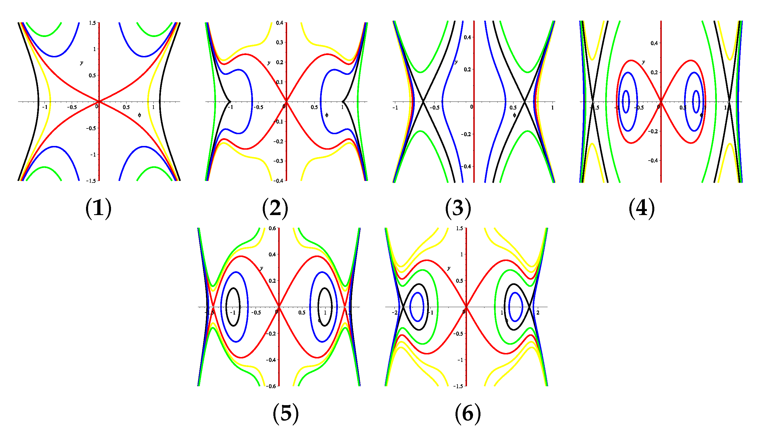
5. Expressions of the Traveling Wave Solutions of System Equation (5) under C > 0 , A = 6 α 8 β

Currently, through integral calculation, we compute the exact parametric expressions of the traveling wave solutions under c > 0 , a = 6 α 8 β . However, in many cases, we cannot find the corresponding solution formulation; here, we only analyze the part where the solution formulation can be found. Because the solution of system (5) in this part is given in the form of a parametric expression, and the calculation process of the exact solution of Equation (1) obtained after the traveling wave transformation is substituted back is too complicated, the exact solution of Equation (1) is not given here. The solution follows from Equation (7) and the first equation of system (5):
ξ = ϕ 0 ϕ d ϕ y ( ϕ ) = ϕ 0 ϕ ± d ϕ 2 c 5 ( 2 α a ) ϕ 6 + 2 b 3 ( 2 α a ) ϕ 4 + 2 ( ω + γ + a κ 2 ) a 2 α ϕ 2 + h ϕ .

5.1. The Parameter Condition of A 2 α > 0 , Δ > 0 , B < 0 , ω + γ + a κ 2 < 0 , H 1 = h 2 < h 0 < h 3 = h 4 (See Figure 5(4))

(i) In formula (7), if H ( ϕ , y ) = h 4 , there are two homoclinic orbits and a periodic orbit. For one of the homoclinic orbits that tangents the singular line ϕ = 0 to E 0 ( 0 , 0 ) , we have y 2 = 2 c 5 ( a 2 α ) ( r 1 ϕ ) ( r 2 ϕ ) ( 0 ϕ ) ϕ + b Δ 2 c 2 ( ϕ r 3 ) . For the other homoclinic orbit, we have y 2 = 2 c 5 ( a 2 α ) ( r 1 ϕ ) ( r 2 ϕ ) ( 0 ϕ ) b Δ 2 c ϕ 2 ( ϕ r 3 ) . For the periodic orbit, we have y 2 = 2 c 5 ( a 2 α ) ( r 1 ϕ ) ( ϕ r 2 ) ϕ ϕ + b Δ 2 c 2 ( ϕ r 3 ) , where r 1 > r 2 > 0 > b Δ 2 c > r 3 . Then, the parametric representations of the traveling wave solution for the homoclinic orbit that contacts the singular line ϕ = 0 at E 0 are given as
ϕ ( χ ) = r 2 r 3 sn 2 ( χ , k 10 ) r 2 r 3 + r 3 sn 2 ( χ , k 10 ) , ξ ( χ ) = β 1 2 α 1 2 g 22 Π ( χ , β 1 2 ) + α 1 2 g 22 χ ,
where α 1 2 = r 3 r 3 r 2 , β 1 2 = r 3 r 2 + b Δ 2 c ( r 3 r 2 ) b Δ 2 c , k 10 2 = r 3 ( r 2 r 1 ) r 1 ( r 2 r 3 ) , g 22 = 1 2 β 1 2 b Δ 2 c 2 c r 1 ( r 2 r 3 ) 5 ( a 2 α ) .
The parametric representations of the traveling wave solution for the other homoclinic orbit are given as
ϕ ( χ ) = r 1 r 3 ( 1 sn 2 ( χ , k 11 ) ) r 1 r 3 sn 2 ( χ , k 11 ) , ξ ( χ ) = β 2 2 α 2 2 g 23 Π ( χ , β 2 2 ) + α 2 2 g 23 χ ,
where β 2 2 = α 2 2 r 1 + b Δ 2 c r 3 + b Δ 2 c , g 23 = 1 2 β 2 2 r 3 + b Δ 2 c 2 c r 1 ( r 2 r 3 ) 5 ( a 2 α ) , α 2 2 = r 3 r 1 , k 11 2 = r 3 ( r 2 r 1 ) r 1 ( r 2 r 3 ) .
The parametric expressions of the traveling wave solution for the periodic orbit are given as
ϕ ( χ ) = r 1 ( r 2 r 3 ) + r 3 ( r 1 r 2 ) sn 2 ( χ , k 12 ) r 2 r 3 + ( r 1 r 2 ) sn 2 ( χ , k 12 ) , ξ ( χ ) = β 3 2 α 3 2 g 24 Π ( χ , β 3 2 ) + α 3 2 g 24 χ ,
where β 3 2 = ( r 2 r 1 ) r 3 + b Δ 2 c ( r 2 r 3 ) r 1 + b Δ 2 c , g 24 = 1 2 β 3 2 r 1 + b Δ 2 c 2 c r 1 ( r 2 r 3 ) 5 ( a 2 α ) , α 3 2 = r 2 r 1 r 2 r 3 , k 12 2 = r 3 ( r 2 r 1 ) r 1 ( r 2 r 3 ) .
(ii) For the curves H ( ϕ , y ) = h 3 , there exist a periodic orbit and two homoclinic orbits. For the periodic orbit, we have y 2 = 2 c 5 ( a 2 α ) ( r 1 ϕ ) b Δ 2 c ϕ 2 ( 0 ϕ ) ( r 2 ϕ ) ( ϕ r 3 ) . For one of the homoclinic orbits that contacts the singular line ϕ = 0 at E 0 ( 0 , 0 ) , we have y 2 = 2 c 5 ( a 2 α ) ( r 1 ϕ ) b Δ 2 c ϕ 2 ϕ ( ϕ r 2 ) ( ϕ r 3 ) . For the other homoclinic orbit, we have y 2 = 2 c 5 ( a 2 α ) ( r 1 ϕ ) ϕ b Δ 2 c 2 ϕ ( ϕ r 2 ) ( ϕ r 3 ) , where r 1 > b Δ 2 c > 0 > r 2 > r 3 . Then, the parametric representations of the traveling wave solution for the periodic orbit are given as
ϕ ( χ ) = r 2 r 3 r 3 + ( r 2 r 3 ) sn 2 ( χ , k 13 ) , ξ ( χ ) = β 4 2 α 4 2 g 25 Π ( χ , β 4 2 ) + α 4 2 g 25 χ ,
where β 4 2 = ( r 2 r 3 ) b Δ 2 c r 3 r 2 b Δ 2 c , g 25 = 1 2 β 4 2 b Δ 2 c r 2 2 c r 3 ( r 2 r 1 ) 5 ( a 2 α ) , α 4 2 = r 3 r 2 r 3 , k 13 2 = r 1 ( r 2 r 3 ) r 3 ( r 2 r 1 ) .
The parametric representations of the traveling wave solution for the homoclinic orbit that contacts the singular line ϕ = 0 at E 0 are given as
ϕ ( χ ) = r 1 r 2 sn 2 ( χ , k 14 ) r 2 r 1 + r 1 sn 2 ( χ , k 14 ) , ξ ( χ ) = β 5 2 α 5 2 g 26 Π ( χ , β 5 2 ) + α 5 2 g 26 χ ,
where α 5 2 = r 1 r 1 r 2 , β 5 2 = r 1 b Δ 2 c r 2 ( r 1 r 2 ) b Δ 2 c , k 14 2 = r 1 ( r 2 r 3 ) r 3 ( r 2 r 1 ) , g 26 = 1 2 β 5 2 b Δ 2 c 2 c r 3 ( r 2 r 1 ) 5 ( a 2 α ) .
The parametric representations of the traveling wave solution for the other homoclinic orbit are given as
ϕ ( χ ) = r 1 r 3 ( sn 2 ( χ , k 15 ) 1 ) r 1 sn 2 ( χ , k 15 ) r 3 , ξ ( χ ) = β 6 2 α 6 2 g 27 Π ( χ , β 6 2 ) + α 6 2 g 27 χ ,
where β 6 2 = r 1 b Δ 2 c r 3 r 3 b Δ 2 c r 1 , g 27 = 1 2 β 6 2 r 1 b Δ 2 c 2 c r 3 ( r 2 r 1 ) 5 ( a 2 α ) , α 6 2 = r 1 r 3 , k 15 2 = r 1 ( r 2 r 3 ) r 3 ( r 2 r 1 ) .

5.2. The Parameter Condition of A 2 α > 0 , Δ > 0 , B < 0 , ω + γ + a κ 2 < 0 , H 1 = h 2 = h 0 < h 3 = h 4 (See Figure 5(5))

(i) In formula (7), if H ( ϕ , y ) = h 4 , there are two homoclinic orbits. For one of the homoclinic orbits that tangents the singular line ϕ = 0 to E 0 ( 0 , 0 ) , we have y 2 = 2 c 5 ( a 2 α ) ( 0 ϕ ) ϕ + b Δ 2 c 2 ( ϕ r 1 ) ( ϕ r 2 ) ( ϕ r 2 ¯ ) , but we do not find a corresponding formulation for solving it.
For the other homoclinic orbit, we have y 2 = 2 c 5 ( a 2 α ) ( 0 ϕ ) b Δ 2 c ϕ 2 ( ϕ r 1 ) ( ϕ r 2 ) ( ϕ r 2 ¯ ) , where b Δ 2 c > r 1 , r 2 and r 2 ¯ are complex. Then, we derive the parametric representations of the traveling wave solution for the homoclinic orbit as follows:
ϕ ( χ ) = r 1 A 2 ( 1 + cn ( χ , k 16 ) ) A 2 + B 2 + ( B 2 A 2 ) cn ( χ , k 16 ) , ξ ( χ ) = g 28 β 7 χ + α 7 β 7 1 α 7 2 Π χ , α 7 2 α 7 2 1 α 7 ( α 7 β 7 ) 2 ( 1 α 7 2 ) α 7 2 1 k 16 2 + ( 1 k 16 2 ) α 7 2 ln k 16 2 + ( 1 k 16 2 ) α 7 2 dn χ + α 7 2 1 sn χ k 16 2 + ( 1 k 16 2 ) α 7 2 dn χ α 7 2 1 sn χ ,
where A 2 2 = r 2 r 2 ¯ , B 2 2 = ( r 1 r 2 ) ( r 1 r 2 ¯ ) , g 28 = A 2 + B 2 A 2 B 2 ( B 2 A 2 ) b Δ 2 c r 1 A 2 5 ( a 2 α ) 2 c , k 16 2 = r 1 2 ( A 2 B 2 ) 2 4 A 2 B 2 , α 7 = r 1 A 2 + ( A 2 B 2 ) b Δ 2 c r 1 A 2 + ( A 2 + B 2 ) b Δ 2 c , β 7 = A 2 B 2 A 2 + B 2 , α 7 2 α 7 2 1 > k 16 2 .
(ii) In formula (7), if H ( ϕ , y ) = h 3 , there are two homoclinic orbits. For one of the homoclinic orbits that tangents the singular line ϕ = 0 to E 0 ( 0 , 0 ) , we have y 2 = 2 c 5 ( a 2 α ) ( r 1 ϕ ) b Δ 2 c ϕ 2 ϕ ( ϕ r 2 ) ( ϕ r 2 ¯ ) , where r 1 > b Δ 2 c > 0 , r 2 and r 2 ¯ are complex. Then, we derive the expressions of the traveling wave solution for the homoclinic orbit as follows:
ϕ ( χ ) = r 1 B 3 ( 1 cn ( χ , k 17 ) ) A 3 + B 3 + ( A 3 B 3 ) cn ( χ , k 17 ) , ξ ( χ ) = g 29 β 8 χ + α 8 β 8 1 α 8 2 Π χ , α 8 2 α 8 2 1 α 8 ( α 8 β 8 ) 2 ( 1 α 8 2 ) α 8 2 1 k 17 2 + ( 1 k 17 2 ) α 8 2 ln k 17 2 + ( 1 k 17 2 ) α 8 2 dn χ + α 8 2 1 sn χ k 17 2 + ( 1 k 17 2 ) α 8 2 dn χ α 8 2 1 sn χ ,
where A 3 2 = ( r 1 r 2 ) ( r 1 r 2 ¯ ) , B 3 2 = r 2 r 2 ¯ , g 29 = A 3 + B 3 A 3 B 3 r 1 B 3 + ( A 3 B 3 ) b Δ 2 c 5 ( a 2 α ) 2 c , k 17 2 = r 1 2 ( A 3 B 3 ) 2 4 A 3 B 3 , α 8 = ( B 3 A 3 ) b Δ 2 c r 1 B 3 r 1 B 3 ( A 3 + B 3 ) b Δ 2 c , β 8 = A 3 B 3 A 3 + B 3 , α 8 2 α 8 2 1 > k 17 2 .
For the other homoclinic orbit, we have y 2 = 2 c 5 ( a 2 α ) ( r 1 ϕ ) ϕ b Δ 2 c 2 ϕ ( ϕ r 2 ) ( ϕ r 2 ¯ ) , but we do not find a corresponding formulation for solving it.

5.3. The Parameter Condition of A 2 α > 0 , Δ > 0 , B < 0 , ω + γ + a κ 2 < 0 , H 0 < h 1 = h 2 < h 3 = h 4 ( S e e F i g u r e ( 6 ) ) (See Figure 5(6))

(i) In formula (7), if H ( ϕ , y ) = h 4 , there are one homoclinic orbit and two heteroclinic orbits that contact the singular line ϕ = 0 at E 0 ( 0 , 0 ) . The traveling wave solutions of these curves are the same as (93).
(ii) In formula (7), if H ( ϕ , y ) = h 3 , there are one homoclinic orbit and two heteroclinic orbits that contact the singular line ϕ = 0 at E 0 ( 0 , 0 ) . The traveling wave solutions of these curves are same as (94).

5.4. The Case of Δ > 0 , ω + γ + a κ 2 > 0 (See Figure 6(3))

For the curves H ( ϕ , y ) = h 1 , there exists a homoclinic orbit, which contacts the singular line ϕ = 0 at E 0 ( 0 , 0 ) . We have y 2 = 2 c 5 ( 2 α a ) b + Δ 2 c ϕ 2 ϕ ( ϕ r 1 ) ( ϕ r 2 ) ( ϕ r 2 ¯ ) , where b + Δ 2 c > 0 > r 1 , r 2 and r 2 ¯ are complex. Then, we derive the expressions of the traveling wave solution for the homoclinic orbit as follows:
ϕ ( χ ) = r 1 A 4 ( 1 cn ( χ , k 18 ) ) A 4 B 4 ( A 4 + B 4 ) cn ( χ , k 18 ) , ξ ( χ ) = g 30 β 9 χ + α 9 β 9 1 α 9 2 Π χ , α 9 2 α 9 2 1 α 9 ( α 9 β 9 ) 2 ( 1 α 9 2 ) α 9 2 1 k 18 2 + ( 1 k 18 2 ) α 9 2 ln k 18 2 + ( 1 k 18 2 ) α 9 2 dn χ + α 9 2 1 sn χ k 18 2 + ( 1 k 18 2 ) α 9 2 dn χ α 9 2 1 sn χ ,
where A 4 2 = r 2 r 2 ¯ , B 4 2 = ( r 1 r 2 ) ( r 1 r 2 ¯ ) , g 30 = A 4 B 4 A 4 B 4 r 1 A 4 ( A 4 + B 4 ) b + Δ 2 c 5 ( 2 α a ) 2 c , k 18 2 = ( A 4 + B 4 ) 2 r 1 2 4 A 4 B 4 , α 9 = r 1 A 4 ( A 4 + B 4 ) b + Δ 2 c ( A 4 B 4 ) b + Δ 2 c r 1 A 4 , β 9 = B 4 + A 4 B 4 A 4 , α 9 2 α 9 2 1 > k 18 2 .

5.5. The Parameter Condition of A 2 α < 0 , Δ > 0 , B < 0 , ω + γ + a κ 2 < 0 , H 3 = h 4 < h 0 < h 1 = h 2 (See Figure 6(5))

(i) For the curves H ( ϕ , y ) = h 2 , there exist a periodic orbit and a homoclinic orbit that contacts the singular line ϕ = 0 at E 0 . For the periodic orbit, we have y 2 = 2 c 5 ( 2 α a ) ( r 1 ϕ ) ( r 2 ϕ ) ( ϕ r 3 ) ϕ ϕ + b + Δ 2 c 2 . For the homoclinic orbit, we have y 2 = 2 c 5 ( 2 α a ) ( r 1 ϕ ) ( r 2 ϕ ) ( r 3 ϕ ) ( 0 ϕ ) ϕ + b + Δ 2 c 2 , where r 1 > r 2 > r 3 > 0 > b + Δ 2 c . Then, the parametric representations of the traveling wave solutions for the periodic orbit are given as
ϕ ( χ ) = r 2 ( r 1 r 3 ) r 1 ( r 2 r 3 ) sn 2 ( χ , k 19 ) r 1 r 3 ( r 2 r 3 ) sn 2 ( χ , k 19 ) , ξ ( χ ) = β 10 2 α 10 2 g 31 Π ( χ , β 10 2 ) + α 10 2 g 31 χ ,
where β 10 2 = ( r 2 r 3 ) r 1 + b + Δ 2 c ( r 1 r 3 ) r 2 + b + Δ 2 c , g 31 = 1 2 β 10 2 r 2 + b + Δ 2 c 2 c r 2 ( r 3 r 1 ) 5 ( a 2 α ) , α 10 2 = r 2 r 3 r 1 r 3 , k 19 2 = r 1 ( r 2 r 3 ) r 2 ( r 1 r 3 ) . The expressions of the traveling wave solution for the homoclinic orbit are presented as
ϕ ( χ ) = r 1 r 3 sn 2 ( χ , k 20 ) r 3 r 1 + r 1 sn 2 ( χ , k 20 ) , ξ ( χ ) = β 11 2 α 11 2 g 32 Π ( χ , β 11 2 ) + α 11 2 g 32 χ ,
where α 11 2 = r 1 r 1 r 3 , β 11 2 = r 1 r 3 + b + Δ 2 c ( r 1 r 3 ) b + Δ 2 c , k 20 2 = r 1 ( r 2 r 3 ) r 2 ( r 1 r 3 ) , g 32 = 1 2 β 11 2 b + Δ 2 c 2 c r 2 ( r 3 r 1 ) 5 ( a 2 α ) .
(ii) For the curves H ( ϕ , y ) = h 1 , there exist a periodic orbit and a homoclinic orbit that contacts the singular line ϕ = 0 at E 0 . For the periodic orbit, we have y 2 = 2 c 5 ( 2 α a ) b + Δ 2 c ϕ 2 ( 0 ϕ ) ( r 1 ϕ ) ( ϕ r 2 ) ( ϕ r 3 ) . For the homoclinic orbit, we have y 2 = 2 c 5 ( 2 α a ) b + Δ 2 c ϕ 2 ϕ ( ϕ r 1 ) ( ϕ r 2 ) ( ϕ r 3 ) , where b + Δ 2 c > 0 > r 1 > r 2 > r 3 . The parametric expressions of the traveling wave solution for the periodic orbit are given as
ϕ ( χ ) = r 1 r 2 r 2 + ( r 1 r 2 ) sn 2 ( χ , k 21 ) , ξ ( χ ) = β 12 2 α 12 2 g 33 Π ( χ , β 12 2 ) + α 12 2 g 33 χ ,
where β 12 2 = ( r 1 r 2 ) b + Δ 2 c r 2 r 1 b + Δ 2 c , g 33 = 1 2 β 12 2 b + Δ 2 c r 1 2 c r 2 ( r 1 r 3 ) 5 ( a 2 α ) , α 12 2 = r 2 r 1 r 2 , k 21 2 = r 3 ( r 1 r 2 ) r 2 ( r 1 r 3 ) . The implicit parametric expression of the traveling wave solution for the homoclinic orbit is given as follows:
ϕ ( χ ) = r 1 r 3 sn 2 ( χ , k 22 ) r 1 r 3 + r 3 sn 2 ( χ , k 22 ) , ξ ( χ ) = β 13 2 α 13 2 g 34 Π ( χ , β 13 2 ) + α 13 2 g 34 χ ,
where α 13 2 = r 3 r 3 r 1 , β 13 2 = r 3 r 1 b + Δ 2 c ( r 1 r 3 ) b + Δ 2 c , k 22 2 = r 3 ( r 1 r 2 ) r 2 ( r 1 r 3 ) , g 34 = 1 2 β 13 2 b + Δ 2 c 2 c r 2 ( r 1 r 3 ) 5 ( a 2 α ) .

5.6. The Parameter Condition of A 2 α < 0 , Δ > 0 , B < 0 , ω + γ + a κ 2 < 0 , H 3 = h 4 < h 1 = h 2 < h 0 (See Figure 6(7))

For the level curves H ( ϕ , y ) = h 1 , there exists a homoclinic orbit to E 1 . We have y 2 = 2 c 5 ( 2 α a ) b + Δ 2 c ϕ 2 ( ϕ r 1 ) ϕ ( ϕ r 2 ) ( ϕ r 2 ¯ ) , where b + Δ 2 c > r 1 > 0 , r 2 and r 2 ¯ are complex. Then, the parametric representations of the traveling wave solution for the homoclinic orbit are given as
ϕ ( χ ) = r 1 B 5 ( 1 + cn ( χ , k 23 ) ) B 5 A 5 + ( A 5 + B 5 ) cn ( χ , k 23 ) , ξ ( χ ) = g 35 β 14 χ + α 14 β 14 1 α 14 2 Π χ , α 14 2 α 14 2 1 α 14 ( α 14 β 14 ) 2 ( 1 α 14 2 ) α 14 2 1 k 23 2 + ( 1 k 23 2 ) α 14 2 ln k 23 2 + ( 1 k 23 2 ) α 14 2 dn χ + α 14 2 1 sn χ k 23 2 + ( 1 k 23 2 ) α 14 2 dn χ α 14 2 1 sn χ ,
where A 5 2 = ( r 1 r 2 ) ( r 1 r 2 ¯ ) , B 5 2 = r 2 r 2 ¯ , g 35 = A 5 B 5 A 5 B 5 r 1 B 5 ( A 5 + B 5 ) b + Δ 2 c 5 ( 2 α a ) 2 c , k 23 2 = ( A 5 + B 5 ) 2 r 1 2 4 A 5 B 5 , α 14 = r 1 B 5 ( A 5 + B 5 ) b + Δ 2 c r 1 B 5 + ( A 5 B 5 ) b + Δ 2 c , β 14 = B 5 + A 5 B 5 A 5 , α 14 2 α 14 2 1 > k 23 2 .

6. Main Results

Based on the above analysis and calculation, we obtain the exact expressions of wave solutions of the FCGL equation. We list them all in the following theorem.
Theorem 1.
The exact expressions of wave solutions of the FCGL equation are as below:
(B1) Corresponding to some periodic orbits, there exist exact periodic wave solutions determined by (17), (23), (24), (33), (39), (54), (58), (62), (64), (72), (89), (90), (96) and (98).
(B2) Corresponding to some homoclinic orbits, there exist exact solitary wave solutions determined by (19), (21), (27), (41), (51), (56), (60), (68), (74), (84), (87), (88), (91)–(95), (97), (99) and (100).
(B3) Corresponding to some heteroclinic orbits, there exist exact kink and anti-kink wave solutions determined by (13), (14), (28), (29), (35), (36), (43)–(46) and (76)–(79).
(B4) Corresponding to some open orbits, there exist exact compacton solutions determined by (65) and (70).

7. Conclusions

In this paper, we investigate the bifurcations and the exact solutions of the time–space fractional complex Ginzburg–Landau equation with parabolic law nonlinearity ( F ( | q | 2 ) = c 1 | q | 2 + c 2 | q | 4 ) . All possible explicit representations of traveling wave solutions are given for the time-space FCGL equation under different parameter domains, including peakon solutions, periodic peakon solutions, compacton solutions, kink and anti-kink wave solutions, solitary wave solutions, periodic wave solutions and so on. Our method is different from the previous works on the exact solutions of the time-space FCGL equation and is based on the applying bifurcation theory of planar dynamical systems.

Author Contributions

Methodology, W.Z. and Y.X.; software, W.Z., Z.L. and M.G.; validation, W.Z., Z.L., Y.X. and M.G.; formal analysis, W.Z., Z.L. and Y.X.; investigation, W.Z., Z.L. and Y.X.; writing—original draft preparation, W.Z. and Z.L.; writing—review and editing, Y.X.; supervision, Y.X. All authors have read and agreed to the published version of the manuscript.

Funding

This work was jointly supported by the National Natural Science Foundation of China under Grant (No. 11901547), and Natural Science Foundation of Zhejiang Province under Grant (No. LQ19A040003).

Data Availability Statement

This manuscript has no associated data.

Acknowledgments

The authors are very grateful to the editors and anonymous reviewers for their constructive comments and suggestions.

Conflicts of Interest

The authors declare no conflict of interest.

References

  1. Weitzner, H.; Zaslavsky, G.M. Some applications of fractional equations. Commun. Nonlinear Sci. and Numer. Simul. 2003, 8, 273–281. [Google Scholar] [CrossRef] [Green Version]
  2. Tarasov, V.E. Fractional dynamics. In Nonlinear Physical Science; Springer: Berlin/Heidelberg, Germany, 2010. [Google Scholar]
  3. Tarasov, V.E.; Zaslavsky, G.M. Fractional Ginzburg-Landau equation for fractal media. Physica A 2005, 354, 249–261. [Google Scholar] [CrossRef] [Green Version]
  4. Abdou, M.A.; Soliman, A.A.; Biswas, A.; Ekici, M.; Zhou, Q.; Moshokoa, S.P. Dark-singular combo optical solitons with fractional complex Ginzburg-Landau equation. Optik 2018, 171, 463–467. [Google Scholar] [CrossRef]
  5. Arshed, S. Soliton solutions of fractional complex Ginzburg-Landau equation with Kerr law and non-Kerr law media. Optik 2018, 160, 322–332. [Google Scholar] [CrossRef]
  6. Fang, J.; Mou, D.; Wang, Y.; Zhang, H.; Dai, C.; Chen, Y. Soliton dynamics based on exact solutions of conformable fractional discrete complex cubic Ginzburg-Landau equation. Results Phys. 2021, 20, 103710. [Google Scholar] [CrossRef]
  7. Li, L.; Jin, L.; Fang, S. Large time behavior for the fractional Ginzburg-Landau equations near the BCS-BEC crossover regime of Fermi gases. Bound. Value Probl. 2017, 2017.1, 1–16. [Google Scholar] [CrossRef] [Green Version]
  8. Lu, H.; Bates, P.W.; Lü, S.; Zhang, M. Dynamics of the 3-D fractional complex Ginzburg-Landau equation. Differ. Equ. 2015, 259, 5276–5301. [Google Scholar] [CrossRef]
  9. Milovanov, A.; Rasmussen, J. Fractional generalization of the Ginzburg-Landau equation: An unconventional approach to critical phenomena in complex media. Phys. Lett. A 2005, 337, 75–80. [Google Scholar] [CrossRef] [Green Version]
  10. Mvogo, A.; Tambue, A.; Ben-Bolie, G.; Kofane, T. Localized numerical impulse solutions in diffuse neural networks modeled by the complex fractional Ginzburg-Landau equation. Commun. Nonlinear Sci. 2016, 39, 396–410. [Google Scholar] [CrossRef]
  11. Pu, X.; Guo, B. Well-posedness and dynamics for the fractional Ginzburg-Landau equation. Appl. Anal. 2013, 92, 318–334. [Google Scholar] [CrossRef]
  12. Qiu, Y.; Malomed, B.A.; Mihalache, D.; Zhu, X.; Zhang, L.; He, Y. Soliton dynamics in a fractional complex Ginzburg-Landau model. Chaos Solitons Frcatals 2020, 131, 109471. [Google Scholar] [CrossRef] [Green Version]
  13. Raza, N. Exact periodic and explicit solutions of the conformable time fractional Ginzburg-Landau equation. Opt. Quant. Electron. 2018, 50, 154. [Google Scholar] [CrossRef]
  14. Sadaf, M.; Akram, G.; Dawood, M. An investigation of fractional complex Ginzburg-Landau equation with Kerr law nonlinearity in the sense of conformable, beta and M-truncated derivatives. Opt. Quantum Electron. 2022, 54, 248. [Google Scholar] [CrossRef]
  15. Zhu, W.; Xia, Y.; Zhang, B.; Bai, Y. Exact traveling wave solutions and bifurcations of the time fractional differential equations with applications. Internat. J. Bifur. Chaos 2019, 29, 1950041. [Google Scholar] [CrossRef]
  16. Chen, A.; Tian, C.; Huang, W. Periodic solutions with equal period for the Friedmann-Robertson-Walker model. Appl. Math. Lett. 2018, 77, 101–107. [Google Scholar] [CrossRef]
  17. Chen, A.; Guo, L.; Huang, W. Existence of kink waves and periodic waves for a perturbed defocusing mKdV equation. Qual. Theory Dyn. Syst. 2018, 17, 495–517. [Google Scholar] [CrossRef]
  18. Sun, X.; Yu, P. Periodic traveling waves in a generalized BBM equation with weak backward diffusion and dissipation terms. Discret. Contin. Dyn. Syst. 2019, 24, 965–987. [Google Scholar] [CrossRef] [Green Version]
  19. Sun, X.; Huang, W.; Cai, J. Coexistence of the solitary and periodic waves in convecting shallow water fluid. Nonlinear Anal. Real World Appl. 2020, 53, 103067. [Google Scholar] [CrossRef]
  20. Ge, J.; Du, Z. The solitary wave solutions of the nonlinear perturbed shallow water wave model. Appl. Math. Lett. 2020, 103, 106202. [Google Scholar] [CrossRef]
  21. Chen, A.; Guo, L.; Deng, X. Existence of solitary waves and periodic waves for a perturbed generalized BBM equation. J. Differ. Equ. 2016, 261, 5324–5349. [Google Scholar] [CrossRef]
  22. Du, Z.; Li, J.; Li, X. The existence of solitary wave solutions of delayed Camassa-Holm equation via a geometric approach. J. Funct. Anal. 2018, 275, 988–1007. [Google Scholar] [CrossRef]
  23. Zhu, K.; Shen, J. Smooth travelling wave solutions in a generalized Degasperis-Procesi equation. Commun. Nonl. Sci. Numer. Simulat. 2021, 98, 105763. [Google Scholar] [CrossRef]
  24. Song, Y.; Tang, X. Stability, Steady-state bifurcations, and turing patterns in a predator-prey model with herd behavior and prey-taxis. Stud. Appl. Math. 2017, 139, 371–404. [Google Scholar] [CrossRef]
  25. Song, Y.; Wu, S.; Wang, H. Spatiotemporal dynamics in the single population modelwith memory-based diffusion and nonlocal effect. J. Differ. Equ. 2019, 267, 6316–6351. [Google Scholar] [CrossRef]
  26. Chen, H.; Duan, S.; Tang, Y.; Xie, J. Global dynamics of a mechanical system with dry friction. J. Differ. Equ. 2018, 265, 5490–5519. [Google Scholar] [CrossRef]
  27. Chen, H.; Li, Z.; Zhang, R. A sufficient and necessary condition of generalized polynomial Liénard systems with global centers. arXiv 2022, arXiv:2208.06184. [Google Scholar]
  28. Chen, H.; Llibre, J.; Tang, Y. Global dynamics of a SD oscillator. Nonlinear Dyn. 2018, 91, 1755–1777. [Google Scholar] [CrossRef] [Green Version]
  29. Chen, H.; Tang, Y. At most two limit cycles in a piecewise linear differential system with three zones and asymmetry. Phys. D Nonlinear Phenom. 2019, 386, 23–30. [Google Scholar] [CrossRef]
  30. Deng, X. Travelling wave solutions for the generalized Burgers-Huxley equation. Appl. Math. Comput. 2008, 204, 733–737. [Google Scholar] [CrossRef]
  31. Li, J. Singular Nonlinear Travelling Wave Equations: Bifurcations and Exact Solutions; Science Press: Beijing, China, 2013. [Google Scholar]
  32. Li, J.; Chen, G. On a class of singular nonlinear traveling wave equations. Int. J. Bifurcation Chaos 2007, 17, 4049–4065. [Google Scholar] [CrossRef]
  33. Li, J.; Qiao, Z. Peakon, pseudo-peakon, and cuspon solutions for two generalized Cammasa-Holm equations. J. Math. Phys. 2013, 54, 123501. [Google Scholar] [CrossRef] [Green Version]
  34. He, B.; Meng, Q.; Long, Y.; Rui, W. New exact solutions of the double sine-Gordon equation using symbolic computations. Appl. Math. Comput. 2007, 186, 1334–1346. [Google Scholar]
  35. Meng, Q.; He, B.; Long, Y.; Rui, W. Bifurcations of travelling wave solutions for a general sine-Gordon equation. Chaos Solitons Fractals 2006, 29, 483–489. [Google Scholar] [CrossRef]
  36. Wen, Z. Bifurcations and exact traveling wave solutions of a new two-component system. Nonlinear Dyn. 2017, 87, 1917–1922. [Google Scholar] [CrossRef]
  37. Wu, L.; He, G.; Geng, X. Quasi-periodic solutions to the two-component nonlinear Klein-Gordon equation. J. Geom. Phys. 2013, 66, 1–17. [Google Scholar] [CrossRef]
  38. Xu, G.; Zhang, Y.; Li, J. Exact solitary wave and periodic-peakon solutions of the complex Ginzburg-Landau equation: Dynamical system approach. Math. Comput. Simul. 2022, 191, 157–167. [Google Scholar] [CrossRef]
  39. Xu, Y.; Zhang, L. Bifurcations of traveling wave solutions for the nonlinear Schrödinger equation with fourth-order dispersion and cubic-quintic nonlieararity. J. Appl. Anal. Comput. 2020, 10, 2722–2733. [Google Scholar]
  40. Zhang, L.; Huang, W. Breaking wave solutions of a short wave model. Results Phys. 2019, 15, 102733. [Google Scholar] [CrossRef]
  41. Zhang, L. Nilpotent singular points and smooth periodic wave solutions. Proc. Rom. Acad. Ser. A 2019, 20, 3–9. [Google Scholar]
  42. Zhu, W.; Xia, Y.; Bai, Y. Traveling wave solutions of the complex Ginzburg-Landau equation with Kerr law nonlinearity. Appl. Math. Comput. 2020, 382, 125342. [Google Scholar] [CrossRef]
  43. Feng, D.H.; Li, J.; Jiao, J. Dynamical behavior of singular traveling waves of (n+1)-dimensional nonlinear Klein-Gordon equation. Qual. Theor. Dyn. Syst. 2019, 18, 265–287. [Google Scholar] [CrossRef]
Figure 1. Phase portraits corresponding to system (5) under c > 0 , α 2 β = 0 , a 2 α > 0 . (1) Δ < 0 or Δ = 0 , b > 0 or Δ > 0 , b > 0 , ω + γ + a κ 2 0 . (2) Δ = 0 , b < 0 . (3) Δ > 0 , ω + γ + a κ 2 > 0 . (4) Δ > 0 , b < 0 , ω + γ + a κ 2 = 0 . (5) Δ > 0 , 3 b 2 16 c < b < 0 , ω + γ + a κ 2 < 0 . (6) Δ > 0 , b = 3 b 2 16 c , ω + γ + a κ 2 < 0 . (7) Δ > 0 , b < 3 b 2 16 c , ω + γ + a κ 2 < 0 .
Fractalfract 07 00201 g001
Figure 2. Phase portraits corresponding to system (5) under c > 0 , α 2 β = 0 , a 2 α < 0 . (1) Δ < 0 or Δ = 0 , b > 0 or Δ > 0 , b > 0 , ω + γ + a κ 2 0 . (2) Δ = 0 , b < 0 . (3) Δ > 0 , ω + γ + a κ 2 > 0 or Δ > 0 , b < 0 , ω + γ + a κ 2 = 0 . (4) Δ > 0 , 3 b 2 16 c < b < 0 , ω + γ + a κ 2 < 0 . (5) Δ > 0 , b = 3 b 2 16 c , ω + γ + a κ 2 < 0 . (6) Δ > 0 , b < 3 b 2 16 c , ω + γ + a κ 2 < 0 .
Fractalfract 07 00201 g002
Figure 3. Phase portraits corresponding to system (5) under c > 0 , ( 2 β α ) ( a 2 α ) > 0 , a 2 α > 0 . (1) Δ < 0 or Δ = 0 , b > 0 or Δ > 0 , b > 0 , ω + γ + a κ 2 0 . (2) Δ = 0 , b < 0 . (3) Δ > 0 , ω + γ + a κ 2 > 0 . (4) Δ > 0 , b < 0 , ω + γ + a κ 2 = 0 . (5) Δ > 0 , b < 0 , ω + γ + a κ 2 < 0 , h 1 = h 2 < h 0 < h 3 = h 4 . (6) Δ > 0 , b < 0 , ω + γ + a κ 2 < 0 , h 1 = h 2 = h 0 < h 3 = h 4 . (7) Δ > 0 , b < 0 , ω + γ + a κ 2 < 0 , h 0 < h 1 = h 2 < h 3 = h 4 .
Fractalfract 07 00201 g003
Figure 4. Phase portraits corresponding to system (5) under c > 0 , ( 2 β α ) ( a 2 α ) > 0 , a 2 α < 0 . (1) Δ < 0 or Δ = 0 , b > 0 or Δ > 0 , b > 0 , ω + γ + a κ 2 0 . (2) Δ = 0 , b < 0 . (3) Δ > 0 , ω + γ + a κ 2 > 0 or Δ > 0 , b < 0 , ω + γ + a κ 2 = 0 . (4) Δ > 0 , b < 0 , ω + γ + a κ 2 < 0 , h 3 = h 4 < h 0 < h 1 = h 2 . (5) Δ > 0 , b < 0 , ω + γ + a κ 2 < 0 , h 3 = h 4 < h 0 = h 1 = h 2 . (6) Δ > 0 , b < 0 , ω + γ + a κ 2 < 0 , h 3 = h 4 < h 1 = h 2 < h 0 .
Fractalfract 07 00201 g004
Figure 5. Phase portraits corresponding to system (5) under c > 0 , ( 2 β α ) ( a 2 α ) < 0 , a 2 α > 0 . (1) Δ < 0 or Δ = 0 , b > 0 or Δ > 0 , b > 0 , ω + γ + a κ 2 0 . (2) Δ = 0 , b < 0 . (3) Δ > 0 , ω + γ + a κ 2 > 0 or Δ > 0 , b < 0 , ω + γ + a κ 2 = 0 . (4) Δ > 0 , b < 0 , ω + γ + a κ 2 < 0 , h 1 = h 2 < h 0 < h 3 = h 4 . (5) Δ > 0 , b < 0 , ω + γ + a κ 2 < 0 , h 1 = h 2 = h 0 < h 3 = h 4 . (6) Δ > 0 , b < 0 , ω + γ + a κ 2 < 0 , h 0 < h 1 = h 2 < h 3 = h 4 .
Fractalfract 07 00201 g005
Figure 6. Phase portraits corresponding to system (5) under c > 0 , ( 2 β α ) ( a 2 α ) < 0 , a 2 α < 0 . (1) Δ < 0 or Δ = 0 , b > 0 or Δ > 0 , b > 0 , ω + γ + a κ 2 0 . (2) Δ = 0 , b < 0 . (3) Δ > 0 , ω + γ + a κ 2 > 0 . (4) Δ > 0 , b < 0 , ω + γ + a κ 2 = 0 . (5) Δ > 0 , b < 0 , ω + γ + a κ 2 < 0 , h 3 = h 4 < h 0 < h 1 = h 2 . (6) Δ > 0 , b < 0 , ω + γ + a κ 2 < 0 , h 3 = h 4 < h 0 = h 1 = h 2 . (7) Δ > 0 , b < 0 , ω + γ + a κ 2 < 0 , h 3 = h 4 < h 1 = h 2 < h 0 .
Fractalfract 07 00201 g006
Figure 7. Kink and anti-kink wave forms of system (5). (a) Kink wave. (b) Anti-kink wave.
Fractalfract 07 00201 g007
Figure 8. Periodic wave forms of system (5). (a) Defined by (17) + . (b) Defined by (17) .
Fractalfract 07 00201 g008
Figure 9. Solitary wave forms of system (5). (a) Bright solitary wave derived by (19) + . (b) Dark solitary wave derived by (19) .
Fractalfract 07 00201 g009
Figure 10. Solitarywave forms of system (5). (a) Bright solitary wave derived by (21) + . (b) Dark solitary wave derived by (21) .
Fractalfract 07 00201 g010
Figure 11. Periodic wave forms of system (5). (a) Defined by (23). (b) Defined by (24) + . (c) Defined by (24) .
Fractalfract 07 00201 g011
Figure 12. Solitarywave forms of system (5). (a) Bright solitary wave derived by (27) + . (b) Dark solitary wave derived by (27) .
Fractalfract 07 00201 g012
Figure 13. Kink and anti-kink wave forms of system (5). (a) Kink wave given by Equation (28). (b) Anti-kink wave given by Equation (29).
Fractalfract 07 00201 g013
Figure 14. Periodicwave forms of system (5).
Fractalfract 07 00201 g014
Figure 15. Kinkand anti-kink wave forms of system (5). (a) Kink wave given by (35). (b) Anti-kink wave given by (36).
Fractalfract 07 00201 g015
Figure 16. Periodic wave forms of system (5). (a) Defined by (39) + . (b) Defined by (39) .
Fractalfract 07 00201 g016
Figure 17. Solitary wave forms of system (5). (a) Bright solitary wave derived by Equation (41) + . (b) Dark solitary wave derived by Equation (41) .
Fractalfract 07 00201 g017
Figure 18. Kink and anti-kink wave forms of system (5). (a) Kink wave given by (43). (b) Anti-kink wave given by (44). (c) Kink wave given by (45). (d) Anti-kink wave given by (46).
Fractalfract 07 00201 g018
Figure 19. Solitary waves forms of system (5). (a) Bright solitary wave derived by (51) + . (b) Dark solitary wave derived by (51) .
Fractalfract 07 00201 g019
Figure 20. Periodicwave forms of system (5). (a) Defined by (54) + . (b) Defined by (54) .
Fractalfract 07 00201 g020
Figure 21. Solitarywave forms of system (5). (a) Bright solitary wave derived by (56) + . (b) Dark solitary wave derived by (56) .
Fractalfract 07 00201 g021
Figure 22. Periodicwave forms of system (5). (a) Defined by (58) + . (b) Defined by (58) .
Fractalfract 07 00201 g022
Figure 23. Solitary wave forms of system (5). (a) Bright solitary wave derived by (60) + . (b) Dark solitary wave derived by (60) .
Fractalfract 07 00201 g023
Figure 24. Periodic wave forms of system (5). (a) Defined by (62) + . (b) Defined by (62) .
Fractalfract 07 00201 g024
Figure 25. Periodic wave forms of system (5). (a) Defined by (64) + . (b) Defined by (64) .
Fractalfract 07 00201 g025
Figure 26. Compactonsolution forms of system (5). (a) Compacton solution given by (65) + . (b) Compacton solution given by (65) .
Fractalfract 07 00201 g026
Figure 27. Solitary wave forms of system (5). (a) Bright solitary wave derived by (68) + . (b) Dark solitary wave derived by (68) .
Fractalfract 07 00201 g027
Figure 28. Compactonsolution forms of system (5). (a) Compacton solution given by Equation (70) + . (b) Compacton solution given by Equation (70) .
Fractalfract 07 00201 g028
Figure 29. Periodic wave forms of system (5). (a) Defined by (72) + . (b) Defined by (72) .
Fractalfract 07 00201 g029
Figure 30. Solitary wave forms of system (5). (a) Bright solitary wave derived by (74) + . (b) Dark solitary wave derived by (74) .
Fractalfract 07 00201 g030
Figure 31. Kink and anti-kink wave forms of system (5). (a) Kink wave given by (76). (b) Anti-kink wave given by (77). (c) Kink wave given by (78). (d) Anti-kink wave given by (79).
Fractalfract 07 00201 g031
Figure 32. Solitary wave forms of system (5). (a) Dark solitary wave derived by (84) + . (b) Bright solitary wave derived by (84) .
Fractalfract 07 00201 g032
Disclaimer/Publisher’s Note: The statements, opinions and data contained in all publications are solely those of the individual author(s) and contributor(s) and not of MDPI and/or the editor(s). MDPI and/or the editor(s) disclaim responsibility for any injury to people or property resulting from any ideas, methods, instructions or products referred to in the content.

